| Issue |
A&A
Volume 660, April 2022
|
|
|---|---|---|
| Article Number | A26 | |
| Number of page(s) | 12 | |
| Section | Extragalactic astronomy | |
| DOI | https://doi.org/10.1051/0004-6361/202142208 | |
| Published online | 04 April 2022 | |
Stochastic gravitational-wave background as a tool for investigating multi-channel astrophysical and primordial black-hole mergers
1
Departement d’Astronomie, Université de Genève, Chemin Pegasi 51, 1290 Versoix, Switzerland
e-mail: This email address is being protected from spambots. You need JavaScript enabled to view it.
2
Département de Physique Théorique and Centre for Astroparticle Physics, Université de Genève, 24 quai E. Ansermet, 1211 Geneva, Switzerland
3
Kavli Institute for Cosmological Physics, The University of Chicago, 5640 South Ellis Avenue, Chicago, Illinois 60637, USA
4
Enrico Fermi Institute, The University of Chicago, 933 East 56th Street, Chicago, Illinois 60637, USA
Received:
13
September
2021
Accepted:
20
December
2021
Abstract
The formation of merging binary black holes can occur through multiple astrophysical channels such as, e.g., isolated binary evolution and dynamical formation or, alternatively, have a primordial origin. Increasingly large gravitational-wave catalogs of binary black-hole mergers have allowed for the first model selection studies between different theoretical predictions to constrain some of their model uncertainties and branching ratios. In this work, we show how one could add an additional and independent constraint to model selection by using the stochastic gravitational-wave background. In contrast to model selection analyses that have discriminating power only up to the gravitational-wave detector horizons (currently at redshifts z ≲ 1 for LIGO–Virgo), the stochastic gravitational-wave background accounts for the redshift integration of all gravitational-wave signals in the Universe. As a working example, we consider the branching ratio results from a model selection study that includes potential contribution from astrophysical and primordial channels. We renormalize the relative contribution of each channel to the detected event rate to compute the total stochastic gravitational-wave background energy density. The predicted amplitude lies below the current observational upper limits of GWTC-3 by LIGO–Virgo, indicating that the results of the model selection analysis are not ruled out by current background limits. Furthermore, given the set of population models and inferred branching ratios, we find that, even though the predicted background will not be detectable by current generation gravitational-wave detectors, it will be accessible by third-generation detectors such as the Einstein Telescope and space-based detectors such as LISA.
Key words: gravitational waves / stars: black holes / black hole physics / dark matter
© ESO 2022
1. Introduction
Coalescing binary black holes (BBHs) are the primary sources of gravitational waves (GWs) that are currently detectable by the LIGO (Aasi et al. 2015), Virgo (Acernese et al. 2015), and KAGRA (Aso et al. 2013) detectors. To date, and only counting events with a false alarm rate of < 1 yr−1, the signals of 69 confident BBH mergers have been reported, along with two binary neutron stars (BNSs) and two black hole–neutron star (BHNS) systems (Abbott et al. 2019, 2021a,b,d,e).
In addition to events that are individually detectable, the entire population of unresolved and resolved events generates a stochastic gravitational-wave background (SGWB) signal. Other than compact binary coalescences, there are multiple astrophysical and cosmological sources contributing to the SGWB. Possible sources include core-collapse supernovae, magnetars, cosmic strings and GWs produced during inflation (e.g., Regimbau 2011; de Freitas Pacheco 2020). However, within the frequency ranges of current GW observatories, the SGWB is thought to be dominated by coalescing compact binaries (Abbott et al. 2016, 2018), whereas BBHs mergers are thought to dominate the SGWB over BNS or BHNS systems (de Freitas Pacheco 2020; Périgois et al. 2021a,b).
The SGWB is characterized by a spectral energy spectrum, ΩGW(ν), which can be measured by cross-correlating the data streams from multiple detectors (Christensen 1992; Allen & Romano 1999). Using the data of the first three observing runs (O1, O2 and O3), the LIGO Scientific and Virgo Collaboration (LVC) did not find evidence of the SGWB. Hence, the LVC was able to put an upper limit to the SGWB energy density spectrum of ΩGW(ν = 25 Hz)≤1.04 × 10⁻⁹ for a power-law SGWB with a spectral index of 2/3, consistent with expectations for coalescing compact binary (Abbott et al. 2021f).
Multiple astrophysical evolutionary pathways may contribute to the formation of coalescing BBHs, which are often divided into categories. The isolated binary evolution family of pathways includes binaries evolving through a stable mass transfer (MT) and a common envelope (CE) phase (e.g., Bethe & Brown 1998; Kalogera et al. 2007; Postnov & Yungelson 2014; Belczynski et al. 2016; Bavera et al. 2020), double stable MT (SMT) (e.g., van den Heuvel et al. 2017; Neijssel et al. 2019; Bavera et al. 2021a), and chemically homogeneous evolution (CHE) (e.g., de Mink et al. 2009; Mandel & de Mink 2016; Marchant et al. 2016; du Buisson et al. 2020). Dynamical formation of BBHs in dense stellar environments may occur in globular clusters (GCs) (e.g., Sigurdsson & Hernquist 1993; Miller & Hamilton 2002; Downing et al. 2010; Rodriguez et al. 2015), nuclear star clusters (NSCs) (e.g., Miller & Lauburg 2009; Petrovich & Antonini 2017; Antonini et al. 2019; Arca Sedda 2020) or young open star clusters (e.g., Ziosi et al. 2014; Mapelli 2016; Banerjee 2017; Kumamoto et al. 2020). Population III stars have also been proposed to lead to merging BBH either in isolation or in a stellar cluster (e.g., Madau & Rees 2001; Kinugawa et al. 2014; Inayoshi et al. 2017; Liu et al. 2021). Furthermore, alternative proposed channels exist, such as the formation of merging BBHs in active galactic nuclei disks (e.g., Antonini & Perets 2012; McKernan et al. 2014; Bartos et al. 2017; Tagawa et al. 2020) and in triple or multiple systems (e.g., Antonini et al. 2016, 2017; Fragione & Loeb 2019; Vigna-Gómez et al. 2021).
Another well-studied formation channel for producing merging BBHs is through a primordial origin (PBHs) (Zel’dovich & Novikov 1967; Hawking 1974; Chapline 1975; Carr 1975), which may arise from the collapse of large overdensities in the radiation-dominated early universe (Ivanov et al. 1994; Garcia-Bellido et al. 1996; Ivanov 1998; Blinnikov et al. 2016) and could contribute to a sizeable ratio fPBH ≡ ΩPBH/ΩDM of the dark matter energy density in a variety of mass ranges (see Carr et al. 2021, for a recent review on constraints on fPBH). The recent discovery of GWs has ignited a new wave of interest in PBHs, particularly as it has been noted that PBHs can produce observable mergers without conflicting with existing bounds on the PBH abundance (Bird et al. 2016; Clesse & García-Bellido 2017; Sasaki et al. 2016). This finding has motivated various works on the confrontation of the PBH scenario with the most recent data (see, e.g., the recent results of Wang et al. 2018, 2019; Hall et al. 2020; Kritos et al. 2021; Hütsi et al. 2021; De Luca et al. 2021b; Deng 2021; Kimura et al. 2021).
Current GW data imply an upper bound of fPBH ≲ 𝒪(10−3) in the mass range of interest for current GW detectors (see e.g., Wong et al. 2021b). The constraining power of GW observations of either resolved mergers or the SGWB will improve significantly with future GW detectors (De Luca et al. 2021c; Pujolas et al. 2021).
All these channels have been shown to successfully lead to the formation of merging BBHs and, in most cases, predict a plausible range of merger-rate density approximately consistent with current GW observational constraints. However, accurate rate estimates are often difficult to be made, as they are highly dependent on uncertain and sometimes unconstrained astrophysical processes. The most well-known uncertainties affecting the astrophysical models include initial stellar and binary properties (e.g., binary ratio, initial mass function, mass ratio and initial orbital parameter distributions), stellar evolution physics (e.g., stellar winds of massive stars, core-collapse mechanism, supernova kicks and pulsational pair instability), binary evolution physics (e.g., MT stability and efficiency, and CE efficiency) as well as uncertainties in the star formation rate and metallicity distribution of their environment at high redshifts (see e.g., Antonini et al. 2017; Chatterjee et al. 2017; Chruslinska et al. 2019; Neijssel et al. 2019; Gröbner et al. 2020; Riley et al. 2021; Belczynski et al. 2022). The primordial channel also suffers from large uncertainties on the overall PBH abundance and initial mass distribution, which are mostly unconstrained in the mass range of interest for LVC mergers (Carr et al. 2021). Combined, these unconstrained physical processes lead to order-of magnitudes uncertainties in the rates, while they often have minor effects on the BBH observable distributions as well (see e.g., Mandel & Broekgaarden 2021, for a review). Such large uncertainties translate to the SGWB energy spectrum and also bias relative ΩGW estimates between channels.
Given the large uncertainty on the modeled BBH rates, comparisons between theoretical predictions and GW observations are often done by normalising the theoretical rate to the observed one. Recent attempts in model selection involving multiple formation channels and GWTC-2 events (Wong et al. 2021a; Zevin et al. 2021a; Franciolini et al. 2021) indicate that given the state-of-the-art formation models considered, multiple formation channels are needed to explain the detected population of BBHs. To date, the work of Zevin et al. (2021a) is the most inclusive analysis accounting for CE, SMT, CHE, GC, and NSC channels. Even though Zevin et al. (2021a) found that a mixture of channels is preferred over a single dominant channel, at face value, the analysis shows that isolated BBH formation might dominate the underlying BBH merging population. It is important to note that only the uncertainties of CE efficiency (cf. Bavera et al. 2021a) and isolated BH spin as a proxy for angular momentum transport were explored in that analysis. The consideration of all model uncertainties and the other prominent BBH formation channel are key to obtaining an unbiased and conclusive answer; however the large number of proposed formation models and model uncertainties, combined with the still limited observational sample, make this task currently computationally infeasible. Following an analysis similar to Zevin et al. (2021a), Franciolini et al. (2021) expanded the set of considered models by also including the PBH channel. The Bayesian evidence in support of PBHs against an astrophysical-only multi-channel model was found to be decisive, due to the fact that the astrophysical models considered there did not produce significant numbers of high-mass events, such as those observed by the LVC. However, the evidence is weakened in the presence of a dominant SMT isolated formation channel, which is more efficient at producing high-mass BBHs.
In this work we compute the contribution to the SGWB energy spectrum of astrophysical and primordial BBHs using the results of the model comparison by Franciolini et al. (2021) as a working example. The relative contribution of each channel is directly dictated by the comparison of the models with the GWTC-2 data, and their total contribution normalized against the BBH detection rate of 44 events, including GW1905211. This assumption is complementary to previous studies which use phenomenological astrophysical models (e.g., Callister et al. 2020; Zhao & Lu 2021) and arbitrarily fix the relative contribution of primordial to astrophysical BBHs (e.g., Chen et al. 2019; Mukherjee & Silk 2021a; Mukherjee et al. 2022). Moreover, our analysis gives a further model constraint to model selection studies as the SGWB includes the rate contribution across all redshift compared to current GW detectors horizons of z ≲ 1 (Abbott et al. 2020a). The results presented in this work are meant to illustrate a methodology that can be applied to and extended toward future catalogs of BBH events, putting more stringent constraints on model selection studies. The best-fit parameters of astrophysical and PBH models, with the corresponding branching ratios, can change drastically with adjustments in the population models or the formation channels considered. However, accounting for the measurement or upper limits on the SGWB provides a new additional constraint on the validity of model selection results, which to our best knowledge is considered here for the first time.
The paper is structured as follows. In Sect. 2, we present the main assumption of each considered astrophysical and primordial BBH channel and explain how we estimate the SGWB energy density spectrum. Section 3 presents the SGWB energy density spectrum of our models compared to current and planned ground- and space-based GW observatories such as the Einstein Telescope (ET) (Punturo et al. 2010) and the Laser Interferometer Space Antenna (LISA) (Amaro-Seoane et al. 2017).
Finally, in Sect. 4 we discuss how our results depend on model uncertainties and we quantify the effect of neglecting other prominent channels. In Sect. 5 we summarise our findings.
2. Methods
We compute the SGWB energy density spectrum of merging BBHs from astrophysical and primordial origins. For the astrophysical channels we include isolated binary evolution evolving through CE and SMT channels and dynamical formation in GC. We adopt BBH models of isolated binary evolution by Bavera et al. (2021a), a GC model by Rodriguez et al. (2019) as released by Zevin et al. (2021a), and a PBH model by Franciolini et al. (2021). The key assumptions of all these models are summarized in Appendix A. More precisely, as favoured by the model comparison with GWTC-2 data in Franciolini et al. (2021) (but also see Zevin et al. 2021a), we use models with isolated BHs birth spins of zero and for the CE channel the model with common envelope efficiency αCE = 5. Here, an αCE value grater than 1 does not mean that other sources of energy partake in the CE ejection, but more likely, it points to an inaccurate assumption of core-envelope boundaries in the αCE − λ parametrization of CE (see, e.g., Ivanova et al. 2013, for a review). The fact that envelope stripping stops earlier than what is currently assumed in population synthesis models has been suggested in multiple recent studies (Fragos et al. 2019; Quast et al. 2019; Klencki et al. 2021; Marchant et al. 2021). Finally, the combined and relative detection rate and (indirectly) the local merger rate density of these channels are calibrated against the model selection comparison of Franciolini et al. (2021) with GWTC-2 events.
For a graphical visualisation of the intrinsic distributions of the main BBH observables of all considered channels, in Fig. 1, we show the underlying distributions of chirp mass ℳ and effective spin parameter χ. The intrinsic (underlying) BBH distribution is what a GW detector with infinite sensitivity would observe on Earth. Here, the chirp mass is defined as ℳ = (m1m2)3/5/(m1 + m2)1/5 where m1 and m2 are the BH masses and the effective spin parameter χ = (m1a1+m2a2)/M · L̂L̂ where a1 and a2 are the BHs dimensionless spins and L̂ is the orbital angular momentum unit vector. The probability density functions (PDFs) of astrophysical channels are constructed using kernel density estimators (KDE) on the BBH discrete model results, while for the PBH channel the PDFs are semi-analytically determined using Eq. (6).
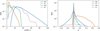 |
Fig. 1. Gravitational-wave observables for the intrinsic distribution of merging BBHs in the Universe for different formation channels according to the legends. Left: normalised chirp mass, ℳ, distributions where we can see that the PBH and GC channels leading to more massive BHs, whereas the maximum BH mass of CE and SMT channels is dictated by pulsational pair instability supernovae. Right: normalised effective spin parameter, χ, distributions where we see that only the CE channel generates a large ratio of positive χ due to tidal spin up, while both the GC and PBH channels lead to a symmetric distribution of χ (allowing for negative values) because of isotropically oriented spins in hierarchical mergers (GC) or uncorrelated spin growth (PBHs). |
In Fig. 1, the maximum ℳ of the isolated binary evolution channels CE and SMT is dictated by pulsational pair instability supernovae (e.g., Fowler & Hoyle 1964; Woosley 2017; Marchant et al. 2019). However, this is not the case for the GC channel since merger products can be retained in the cluster and merge again. Generally, PBHs form from the collapse of large overdensities in the early universe and their mass is related to the mass contained in the cosmological horizon at the time of collapse. For this reason, PBHs can form within a much wider range of masses compared to astrophysical BHs, and they can cover the mass gap (e.g., De Luca et al. 2021a). Even though we assume astrophysical BHs are born with zero spin in isolation, tidal interactions in the later phase of close BH-Walf-Rayet systems can tidally spin up second born BHs in the CE and SMT channels (e.g., Qin et al. 2018; Bavera et al. 2020). The spin of the resultant BH is mostly aligned with the orbital angular momentum since BH natal kicks are not typically strong enough to flip the orbits by more than 90° (e.g., Rodriguez et al. 2016; Callister et al. 2021). Hence, the minimum effective spin parameter of CE and SMT channels is χ ≃ 0. In contrast, GC channel might lead to negative χ given the random dynamical assembly of the BBH systems. Since the majority of these systems are the results of first-generation mergers whose components do not proceed through tidal spinup, the effective spin distribution peaks at χ ≃ 0. However, merger products retained in the cluster are imparted spin due to the angular momentum of the inspiraling binary and, thus, hierarchical mergers lead to a symmetric distribution of χ about zero. While PBHs form with negligible spin in the standard scenario, efficient accretion can spin up PBHs along independent directions and lead to large magnitudes for χ symmetrically distributed around zero (more details in Appendix A.2).
The SGWB energy density spectrum, ΩGW, for each model as well as the GW detectors’ power-law-integrated sensitivity curves are calculated as explained in the following sections.
2.1. SGWB energy density spectrum
Under the cosmological assumption of the ΛCDM model, the fractional energy density content of the Universe today is dominated by matter, Ωm ≃ 0.307, and dark energy, ΩΛ ≃ 1 − Ωm. These energy density ratios are defined in terms of closure density  with a current Universe relative rate of expansion H0 = 67 km s−1 Mpc−1 (Planck Collaboration XIII 2016).
In comparison, the energy density ratio of the SGWB, ΩGW, is small and often expressed as a spectrum, namely as a function of frequency. This is done in order to compare it with GW detectors’ power-law-integrated sensitivity curves which are frequency-dependent. Here, we consider frequencies of current and future ground-based detectors such as LIGO, Virgo, KAGRA, and ET, which are sensitive to the [1, 103] Hz band, as well as space-based detectors such as LISA, which are sensitive to [10−4, 0.1] Hz. In such bands, the spectral GW energy density is dominated by merging BBHs (de Freitas Pacheco 2020; Périgois et al. 2021a).
The SGWB spectral energy density ratio is defined as (e.g., Zhu et al. 2011)
 (1)
(1)
where νobs is the observed GW frequency related to the source frame by ν = νobs(1 + z), Fν is the GW spectral energy density and c the speed of light. Here, we can apply the expression:
 (2)
(2)
where dR/dz is the differential GW event rate given by each BBH formation channel (see Sects. 2.2 and 2.3 for astrophysical and primordial models, respectively) and fν is the energy flux per unit frequency emitted by a source at a luminosity distance dL(z), which is related to the comoving distance,  ; here
  , via the relation dL(z) = (1 + z) dc(z).
The integration limit  is given by the maximal emitting GW frequency νcut. Next, we have:
 (3)
(3)
where we use the coordinate transformation dν/dνobs = (1 + z) to change from the observer frame to source frame of reference. Here, dE/dν is the GW energy spectrum emitted by the BBH system evaluated in the source frame. Assuming the BBH systems are in quasi-circular orbits when they reach the [10−4, 103] Hz band, we approximate dE/dν using Eq. (B.1) and the waveform approximations for non-precessing spinning BBHs by Ajith et al. (2011), as explained in Appendix B. Ignoring the precession of spins in the waveforms approximation will not affect our results as the majority of spins in the considered channels are small. In Fig. 2, we show the GW energy spectrum dE/dν for BBH systems with varying component masses and χ.
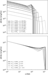 |
Fig. 2. Gravitational-wave energy spectrum, dE/dν, as a function of frequency. Top: energy spectrum for different non-spinning equal mass BBHs according to the legend. The more massive the BBH systems, the more energetic the GW signals and the smaller the merger frequencies. More precisely, the GW energy spectrum scales as dE/dν ∝ ν−1/3ℳ5/3 for ν < νmerger and dE/dν ∝ ν2/3ℳ5/3 for ν < νringdown (cf. Eq. (B.1)), while νmerger ∝ M−1 where M = m1 + m2 is the total mass (cf. Eq. (B.4)). Bottom: energy spectrum for a BBH system composed of two BHs of mass 10 M⊙ and different effective spins according to the legend. Larger χ values lead to more energetic GW signals as dE/dν ∝ ν−1/3(1 + 𝒪χ)) for ν < νmerger and dE/dν ∝ ν2/3(1 + 𝒪χ)) for ν < νringdown (cf. Eq. (B.1)). |
2.2. Astrophysical binary black hole merger rates
For each astrophysical channel, we define  to be the contribution of a binary k to the intrinsic GW event rate (cf. e.g., Bavera et al. 2020, 2022, 2021a)2. This binary is described by component masses m1, k and m2, k and spin vectors a1, k and a2, k. Each binary is placed at the cosmic time bin Δti with its redshift of formation zf, i at the center of the bin, and merges at redshift zm, i, k for its corresponding metallicity bin ΔZj. Here, the “intrinsic” superscript indicates that we assume an infinite detector sensitivity and thus detection probabilities of pdet, i, k = 1, following the notation of Eq. (D.4) in Bavera et al. (2022). Therefore, the BBH event rate observed on Earth for a detector with infinite sensitivity is
  . We can thus calculate the SGWB energy density spectrum of Eq. (1), given any arbitrary intrinsic event rate normalisation N′, as
 (4)
(4)
where  is the normalized cosmological weight. The normalisation constants N′ are given by the model selection result of Franciolini et al. (2021). For each considered astrophysical channel we have a median intrinsic event rate value for the Universe observed on Earth of
  ,
,  and
and  , respectively.
Similar to the BBH event rates, we can calculate the BBH rate density by dividing the normalized cosmological weight contribution of the binary k by the integrated differential comoving volume over Δzi corresponding to the comic time bin Δti, namely:
![Mathematical equation: $$ \begin{aligned} \mathcal{R} (z) = N^{\prime } \sum _{\Delta Z_j, k} \tilde{{ w}}_{i,j,k}^\mathrm{intrinsic} / \Delta V_\mathrm{c} (z_i) \,\,\, [\mathrm{Gpc} ^{-3}\mathrm{yr} ^{-1}] , \end{aligned} $$](/articles/aa/full_html/2022/04/aa42208-21/aa42208-21-eq15.gif) (5)
(5)
where  as in Eq. (D.2) of Bavera et al. (2022).
2.3. Primordial binary black hole merger rate
For the computation of the rate density of binaries in the primordial model, we closely follow the parametrization of the merger rate as in Franciolini et al. (2021) and references therein. We refer to Appendix A.2 for more details on the predictions of the PBH scenario.
Depending on the initial abundance fPBH and mass function ψ(m), one can estimate the probability of forming binaries in the early Universe due to PBHs decoupling from the Hubble flow. The initial distribution of orbital parameters is defined by the spatial distribution of the surrounding population of PBHs, as well as density perturbations adding an initial torque to the binary system (see e.g., Ali-Haïmoud et al. 2017). Then, we compute the differential PBH merger rate density as a function of masses using (De Luca et al. 2020b)
 (6)
(6)
where M = m1 + m2, μ = m1m2/M, η = μ/M, t is the cosmic time and t0 is the current age of the Universe. Integrating Eq. (6) in both masses provides the PBH merger rate density as a function of redshift which we adopt in the following. This formula also accounts for the corrective factors introducing the evolution of PBH masses from the initial redshift zi (i generally indicates high-z quantities before PBH accretion took place) to the cut-off redshift zcut − off and the shrinking of the binary semi-major axis due to accretion (De Luca et al. 2020b). This effect drives the binary evolution up to zcut − off, after which the binary evolves through the energy loss induced by GW emission (Peters & Mathews 1963). The suppression factor S(Mtot, fPBH, ψ)≡S1 × S2 accounts for both the effect of surrounding DM matter inhomogeneities (not in the form of PBHs) and the disruption of binaries due to interactions with neighbouring PBHs (Raidal et al. 2019; Vaskonen & Veermäe 2020; Young & Hamers 2020; Jedamzik 2021b, 2020; De Luca et al. 2020a; Tkachev et al. 2020; Hütsi et al. 2021). In particular, the second component S2, specifically includes the effect of disruption of PBH binaries in early sub-structures formed throughout the history of the universe3. The two components are expressed as (Hütsi et al. 2021):
![Mathematical equation: $$ \begin{aligned}&S_1 (M, f_{\mathrm{PBH} }, \psi ) \thickapprox 1.42 \left( \frac{\langle m^2 \rangle /\langle m\rangle ^2}{\bar{N}({ y}) +C} + \frac{\sigma ^2_{\rm M}}{f^2_{\mathrm{PBH} }}\right) ^{-21/74} \exp \left( - \bar{N} \right) ,\nonumber \\&S_2 (x) \thickapprox \mathrm{min} \left[ 1, 9.6 \cdot 10^{-3} x ^{-0.65} \exp \left( 0.03 \ln ^2 x \right) \right], \end{aligned} $$](/articles/aa/full_html/2022/04/aa42208-21/aa42208-21-eq18.gif) (7)
(7)
with x ≡ fPBH(t(z)/t0)0.44 and the number of neighbouring PBHs being  . The constant C appearing in Eq. (7) is defined in Eq. (A.5) of Hütsi et al. (2021). We note that for fPBH ≲ 0.003, we can always finds S2 ≃ 1, that is, the suppression of the merger rate due to disruption inside PBH clusters is negligible. This is supported by the results obtained through a cosmological N-body simulation finding that PBHs are essentially isolated for a small enough values of the abundance (Inman & Ali-Haïmoud 2019). Therefore, for the small values of fPBH adopted in our analysis following Franciolini et al. (2021), the clustering of PBHs does not play a significant role (Inman & Ali-Haïmoud 2019; Vaskonen & Veermäe 2020; De Luca et al. 2020a).
In order to compute the SGWB energy density ΩGW(νobs) emitted by the PBH population, we calculate the differential merger rate as a function of redshift as:
 (8)
(8)
and we feed this information into Eqs. (1) and (2). Finally, the energy spectrum dE/dν is computed by integrating over the distribution of PBH binary masses as implied by Eq. (6). Also in this case, consistently with the previous section, the PBH model hyper-parameters (i.e., [Mc, σ] determining the PBH mass distribution, the abundance fPBH and zcut − off characterising PBH accretion, more details in Appendix A.2) are assumed to be given by the population inference result of Franciolini et al. (2021). In particular, we adopt Mc = 34.54 M⊙, σ = 0.41, fPBH = 10−3.64 and zcut − off = 23.90, such that the PBH channel is adequate in explaining around (1 − 21)% of the detectable events in the O1/O2/O3a run of LVC, and given the associated astrophysical models considered, the mass gap event GW190521.
2.4. Power-law-integrated sensitivity curves
The power-law-integrated (PI) sensitivity curve of a given detector (Thrane & Romano 2013) can be computed once the noise spectral density and the averaged overlap functions are known following the procedure detailed in Appendix C. For the extended LVC network, we assume instrumental noise in different detectors to be uncorrelated. For triangular detectors we take into account the fact that the three nested inteferometers have correlated noise. All PI sensitivity curves are computed using the public code schNell (Alonso et al. 2020). We choose a (optimistic) signal-to-noise (S/N) threshold of ρ = 2 to claim a detection, as is commonly done in the literature on the subject (see e.g., Périgois et al. 2021a). We note that the PI sensitivity curves scale linearly with ρ (see Eq. (C.8)).
The currently accepted model for the power spectral density of the LISA noise (for both auto and cross-correlations) is based on the Payload Description Document, and is referenced in the LISA Strain Curves document LISA-LCST- SGS-TN-0014.
For ET, it feasible to argue that any estimate of correlated noise is quite arbitrary at the moment. We assume that the noise in ET is 20% correlated between detectors with an arm in common. This means that magnetic noise lies about a factor of 2 in amplitude below other instrument noise. This is a robust assumption at lowest frequencies (< 20 Hz). At higher frequencies, if we consider the subtraction of magnetic noise, the correlation is expected to be substantially less than 20%. It is difficult to predict how much magnetic noise can be removed from the data with subtraction, but it could even involve another factor if 10 in amplitude. A level of correlation of 20% is therefore quite conservative. As the site for ET has not yet been chosen, we arbitrarily chose a location in Sardinia, close to one of the surveyed sites (see Alonso et al. 2020 for the specific coordinates and orientation angle of the triangular network). We used the sensitivity curve of the instrument in the so-called D-configuration (Hild et al. 2011). The resulting PI sensitivity curve is in quantitative agreement with the one of Maggiore et al. (2020).
3. Results
We computed the SGWB of astrophysical and primordial BBHs models based on the relative event rate contribution determined by the model selection comparison against GWTC-2 events of Franciolini et al. (2021). For each channel, in Fig. 3, we show the BBH merger rate density as a function of redshift as well as their combination. Given our event rate normalisation against the observed 44 events of GWCT-2, the modeled combined local rate density is consistent with the LVC redshift-dependent estimation at  (Abbott et al. 2021c)5. For comparison, in Fig. 3, we also plot the assumed SFR density of the Universe. The rate density redshift evolution of the CE and SMT channels follow the SFR density. The GC BBH rate density does not mimic the star formation history of the host galaxies, instead peaking at z ∈ [2, 3] (see e.g., Rodriguez & Loeb 2018). In contrast to the astrophysical channels, primordial BBHs have a monotonically increasing merger rate density with redshift as (Ali-Haïmoud et al. 2017; Raidal et al. 2019; De Luca et al. 2020b)
 (9)
(9)
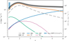 |
Fig. 3. Binary black hole rate density evolution normalised to the model selection results of Franciolini et al. (2021) compared to the local merger rate density inferred from GWTC-2 events assuming a power-law evolution of the merger rate with redshift. We show, in black, the contribution of all channels with relative Poisson error, in gray, computed on the detection rate of the 44 confident BBH events in the O1/O2/O3a observing runs. The model prediction can be directly compared to the local rate constrained by GWTC-2 displayed in blue. With different colors we show the contribution of each channel: common envelope (CE), stable mass transfer (SMT), globular cluster (GC) and primordial black holes (PBH). For comparison, we show the assumed SFR for isolated BBHs which the CE and SMT channels follow, in dashed gray. |
extending up to redshifts z = 𝒪(103). We note that the evolution of the merger rate with time shown in Eq. (9) is entirely determined by the binary formation mechanism (i.e., how pairs of PBHs are decoupled from the Hubble flow) before the matter-radiation equality era. Thus, Eq. (9) serves as a robust prediction of the PBH model, assuming the standard formation scenario where PBHs are generated with an initial spatial Poisson distribution. In our case, given the local normalisation we assume, the PBH contribution grows to overcome the rate density of the astrophysical channels at high redshift (z > 9.5). In contrast, the BBH merger rate density at low redshifts is dominated by the CE and SMT channels up to z = 2, where the PBH and GC dominate over SMT. The SMT channel shows a stronger rate suppression over redshift compared to the CE channel as their delay times, namely, the time between binary formation and BBH merger, are much longer. This occurs because the second MT episode is not as efficient as the CE phase to shrink the BH-Wolf-Rayet binary systems progenitors of the BBHs (Bavera et al. 2021a).
The SGWB energy density spectrum of astrophysical and primordial BBH channels is shown in Fig. 4. Even though the BBH merger rate density is dominated by the CE channel up to redshifts z ≃ 9.5, we find that ΩGW is dominated by the PBH channel in the frequency range ν ∈ [10−4, 400] Hz. The dominance of the PBH channel over astrophysical channels is explained by two factors. First, contrary to the astrophysical channels, the merger rate density of primordial BBHs is a monotonic increasing function (see Fig. 3) peaking at high redshifts of z ≳ 9.5. Second, given the model inference results of Franciolini et al. (2021), primordial BBHs are more massive than those produced by the astrophysical channels (see Fig. 1) whose coalescence will lead to more energetic GW signals (see Fig. 2). The combinations of these two factors leads to the dominance of the PBH channel in the SGWB since ΩGW accounts for the integration over all redshifts. Furthermore, we find that the astrophysical channels dominate ΩGW at ν ∈ [400, 1100] Hz. The suppression of ΩGW at higher frequencies is explained by the fact that the astrophysical channels can produce less massive BBHs compared to our fiducial PBH model (see Fig. 1). Given that the inspiral and merger frequency scale as νmerger ∝ M−1 (cf. Eq. (B.4), but also see Fig. 2), the astrophysical channels contribute to ΩGW above the PBH channel frequency turning point.
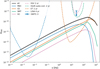 |
Fig. 4. Stochastic gravitational-wave background energy density spectrum of merging astrophysical and primordial BBHs (solid lines). The fiducial model assumes combined BBH event rate normalized against the 44 confident BBH detections of GWTC-2 and branching ratios of each channel inferred by the model selection analysis of Franciolini et al. (2021). We show with individual lines the partial contribution of each channel: common envelope (orange), stable mass transfer (green), globular cluster (pink) and primordial black holes (blue). The total SGWB is indicated in black where the gray band indicates the Poisson error. The upper constraint to the SGWB from GWTC-3 is indicated with a blue bar marker and an arrow. For comparison, we indicate with dashed lines the PI sensitivity curves of different detectors for corresponding continuous observation time. The detector configurations include LIGO-Virgo at design sensitivity (HLV), the same configuration including KAGRA with auto-correlations (HLVK auto-corr.), Einstein Telescope (ET) and the Laser Interferometer Space Array (LISA). |
Our model predicts6
 , roughly ten times smaller than the current observational upper limits by the LVC of ΩGW(ν = 25 Hz)≤1.04 × 10⁻⁹ (Abbott et al. 2021f). We note that this is not a trivial result generated by our normalisation assumption but rather a new constraint to model selection since these SGWB estimates include the integration over all redshifts whereas the constraints from GW events only probe the models up to the detectors horizons (z ≲ 1). Furthermore, we can predict whether our BBH SGWB estimate will be detected by future GW observing runs. To this end, in Fig. 4, we show the PI sensitivity curves for the ground base detectors LIGO-Virgo (HLV) and LIGO-Virgo-KAGRA (HLVK) with auto-correlations and ET accounting for 2 yr of integrated data collection at their design sensitivities as well as the space-based detector LISA for the nominal 4 yr mission. Given our model assumptions, we find that the SGWB of merging BBH lies below the current generation of GW detectors. However, we find that LISA and the third-generation (3G) GW detectors such as ET will be able to detect the BBH SGWB.
4. Discussion
Compared to the analysis of Zevin et al. (2021a), we can see that in Franciolini et al. (2021) the CHE channel was excluded, while the inclusion of the NSC channel was not found to lead to a grater Bayesian evidence, while still managing to reach similar conclusions regarding the relative contributions of CE, SMT, and GC channels. This is due to the CHE and NSC models contributing < 8% and < 13%, respectively, to the underlying merging BBH distribution in Zevin et al. (2021a) at a credibility of 95%. More precisely, the CHE channel mostly leads to highly spinning and massive BHs which are favoured due to GW detector selection effects, and, thus, a smaller contribution to the underlying BBH distribution is required to explain the events in GWTC-2. A similar argument can be made for the NSC channel where in contrast to CHE channel BH spins are smaller. Given the small predicted contribution of these two channels to the intrinsic merger rate distribution we expect a subdominant contribution to ΩGW that is much smaller than the GC contribution in Fig. 4; hence, it will not affect our results.
Our analysis neglects the contribution from the population of non-merging binaries, which previous studies on isolated binary evolution (Périgois et al. 2021a) have found to be negligible compared to the merging population in the frequency bands we consider here. Furthermore, we also did not include eccentric corrections to the GW energy spectrum and assumed that the BBHs would reach the LISA or ground based detector sensitive frequencies with quasi-circular orbits. Périgois et al. (2021a,b) showed that this is the case for isolated binary evolution, while a number of semi-analytic and numerical studies (Breivik et al. 2016; Samsing & Ramirez-Ruiz 2017; Rodriguez et al. 2018; Samsing & D’Orazio 2018; Zevin et al. 2019, 2021b) have shown that for dynamically formed systems a sizable fraction of the BBH population can retain appreciable eccentricity when they enter the LIGO or LISA bands. However, since the GC channel shows a subdominant contribution to the total ΩGW at one part in 20 at ν = 3 mHz, any boost to the GW background from this channel will not change our conclusion significantly.
In this work, we present our SGWB analysis as an additional constraint to multi-channel Bayesian model selection where ΩGW is computed a posteriori to be much smaller than the observational constraint. Alternatively, if we had a more stringent constraint to ΩGW, it would be possible to include the SGWB constraint in the inference of such model selection frameworks, providing the analysis with a direct discriminatory power to models overpredicting ΩGW. Since, in our analysis the SGWB is found to be much smaller than the LVC observational constraint, the result of our model selection would remain the same. On a similar point, based on a phenomenological model, Callister et al. (2020) recently used the SGWB and data on individually resolvable events from O1 and O2 to place joint constraints on the BBH merger rate density peak and slope for low redshifts. We note that the two analyses are complementary, as the one presented here simultaneously constrains the potential contribution of each channel to the total BBH merger rate density; while Callister et al. (2020) puts a direct constraints on the overall joint merger rate density.
A future detection of the SGWB would also possibly help in distinguishing between astrophysical and primordial channels through the SGWB anisotropies (Wang & Kohri 2021). Another example for distinguishing between channels is that in the case where the GC channel dominates the SGWB, we would expect to be able to identify a cusp in ΩGW in the LISA frequency band (D’Orazio & Samsing 2018). Other possible ways to discriminate among different channels is the measurement of the merger bias at 3G detectors via the study of the cross-correlation with the large scale structure (Cusin et al. 2017, 2018; Scelfo et al. 2018; Mukherjee & Silk 2020, 2021b; Calore et al. 2020; Yang et al. 2021), the study of the time evolution of the high redshift merger rates (De Luca et al. 2021b; Ng et al. 2021), and the reconstruction of the spectral shape pre-merger via small band searches.
5. Conclusions
With the aim of further constraining multi-channel BBH Bayesian model selection, as a working example in this work, we computed the SGWB of an astrophysical and primordial BBH population resulting from a model selection comparison with GWTC-2. Because our study did not include all potentially prominent channels leading to merging BBHs and did not span all model uncertainties (cf. Sect. 1), the results of the analysis need to be interpreted with care. Rather than serving as a definitive answer to the question of which channel dominates the SGWB, our analysis is intended to provide a complementary tool to model selection that can be used to further constrain the contribution of particular formation channels. In principle, it provides an additional constraint to model selection as the SGWB probes the theoretical prediction over all redshifts. This is in contrast to model selection analyses that focus on the resolved population, which have discriminating power only up to the GW detector horizons, currently at z ≲ 1 for LIGO–Virgo. Our methodology can therefore be extended to all future model selection studies aiming to unravel the origin of merging BBHs independently from which channel dominates the BBH merger rate density.
To mitigate the high model uncertainties on the merger rate density estimation of each channel that are directly correlated with ΩGW, we normalized the event rate to the 44 confident detections of GWTC-2 and the relative contribution of each channel to the branching ratio results in the model selection analysis of Franciolini et al. (2021). We predict a SGWB of  which lies below the current observational upper limits published by the LVC. Moreover, we find that such background will be accessible only to 3G GW observatories such as ET and the space-based detector LISA.
Finally, with 3G Earth-based detectors, a catalog of individual events and background mapping can provide complementary information on the underlying source population. Combining the two approaches can be useful in gaining information on a high redshift population of sources that cannot be detected and studied individually, even with large-horizon instruments.
Following Abbott et al. (2021c), Franciolini et al. (2021) discarded from the GWTC-2 catalog the events with large false-alarm rates (GW190426, GW190719, GW190909) and two events involving neutron stars (GW170817, GW190425). Also, as the secondary mass (m2 ≈ 2.6 M⊙) of GW190814 (Abbott et al. 2020b) would correspond to either the lowest-mass astrophysical BH or to the highest-mass NS observed to date, challenging current understanding of compact objects, it was assumed that the secondary component of GW190814 is a neutron star and this event was neglected. We notice, however, that its inclusion would not affect our conclusions (Franciolini et al. 2021).
For the GC model (Rodriguez et al. 2019) we take the weights as released by Zevin et al. (2021a) where we divide out the coefficient  and multiplied each weight by ΔVc(zi) to obtain
  .
.
Recent numerical results on PBH clustering confirm the suppression factors we adopt taking into account that the ratio of PBH binaries not entering in clusters is sizeable (Jedamzik 2021a).
We stress that some care has to be taken when comparing different PI sensitivity curves in the literature, as different references assume different arm length for LISA, different observation times and different S/N threshold ρ. We consider the official configuration with 2.5 Gm arms and 4 yr of activity. Our results for the PI agree with Fig. 11 of Babak et al. (2021).
We note that the new GWTC-3 rate estimate 17.3 − 45 Gpc−3 yr−1 at z = 0.2 is consistent with the GWTC-2 estimate (Abbott et al. 2021f).
We report the value of ΩGW at ν = 25 Hz where the current LVC sensitivity has its maximum, see Fig. 4.
In the literature, other PBH mass functions were also considered (e.g., Kühnel & Freese 2017; Bellomo et al. 2018; Hall et al. 2020; Gow et al. 2022). In this work, we follow Franciolini et al. (2021) and adopt Eq. (A.1).
Acknowledgments
The authors would like to thank Valerio De Luca for useful discussions on early stages of the project. This work was supported by the Swiss National Science Foundation Professorship grant (project number PP00P2 176868). G.F. and A.R. are supported by the Swiss National Science Foundation (SNSF), project The Non-Gaussian Universe and Cosmological Symmetries, project number: 200020-178787. The work of G.C. is supported by SNSF Ambizione grant – Gravitational waves propagation in the clustered universe. M.Z. is supported by NASA through the NASA Hubble Fellowship grant HST-HF2-51474.001-A awarded by the Space Telescope Science Institute, which is operated by the Association of Universities for Research in Astronomy, Inc., for NASA, under contract NAS5-26555.
References
- Aasi, J., Abbott, B. P., Abbott, R., et al. 2015, CQG, 32, 074001 [Google Scholar]
- Abbott, B. P., Abbott, R., Abbott, T. D., et al. 2016, Phys. Rev. Lett., 116, 131102 [NASA ADS] [CrossRef] [Google Scholar]
- Abbott, B. P., Abbott, R., Abbott, T. D., et al. 2018, Phys. Rev. Lett., 120, 091101 [CrossRef] [Google Scholar]
- Abbott, B. P., Abbott, R., Abbott, T. D., et al. 2019, Phys. Rev. X, 9, 031040 [Google Scholar]
- Abbott, R., Abbott, T. D., Abraham, S., et al. 2020a, Phys. Rev. Lett., 125, 101102 [Google Scholar]
- Abbott, R., Abbott, T. D., Abraham, S., et al. 2020b, ApJ, 896, L44 [Google Scholar]
- Abbott, R., Abbott, T. D., Abraham, S., et al. 2021a, ApJ, 915, L5 [NASA ADS] [CrossRef] [Google Scholar]
- Abbott, R., Abbott, T. D., Abraham, S., et al. 2021b, Phys. Rev. X, 11, 021053 [Google Scholar]
- Abbott, R., Abbott, T. D., Abraham, S., et al. 2021c, ApJ, 913, L7 [NASA ADS] [CrossRef] [Google Scholar]
- Abbott, R., Abbott, T. D., Acernese, F., et al. 2021d, ArXiv e-prints [arXiv:2108.01045] [Google Scholar]
- Abbott, R., Abbott, T. D., Acernese, F., et al. 2021e, ArXiv e-prints [arXiv:2111.03606] [Google Scholar]
- Abbott, R., Abbott, T. D., Acernese, F., et al. 2021f, ArXiv e-prints [arXiv:2111.03634] [Google Scholar]
- Acernese, F., Agathos, M., Agatsuma, K., et al. 2015, CQG, 32, 024001 [NASA ADS] [CrossRef] [Google Scholar]
- Ajith, P., Hannam, M., Husa, S., et al. 2011, Phys. Rev. Lett., 106, 241101 [NASA ADS] [CrossRef] [Google Scholar]
- Ali-Haïmoud, Y. 2018, Phys. Rev. Lett., 121, 081304 [CrossRef] [Google Scholar]
- Ali-Haïmoud, Y., Kovetz, E. D., & Kamionkowski, M. 2017, Phys. Rev. D, 96, 123523 [CrossRef] [Google Scholar]
- Allen, B., & Romano, J. D. 1999, Phys. Rev. D, 59, 102001 [NASA ADS] [CrossRef] [Google Scholar]
- Alonso, D., Contaldi, C. R., Cusin, G., Ferreira, P. G., & Renzini, A. I. 2020, Phys. Rev. D, 101, 124048 [NASA ADS] [CrossRef] [Google Scholar]
- Amaro-Seoane, P., Audley, H., Babak, S., et al. 2017, ArXiv e-prints [arXiv:1702.00786] [Google Scholar]
- Antonini, F., & Perets, H. B. 2012, ApJ, 757, 27 [NASA ADS] [CrossRef] [Google Scholar]
- Antonini, F., Chatterjee, S., Rodriguez, C. L., et al. 2016, ApJ, 816, 65 [NASA ADS] [CrossRef] [Google Scholar]
- Antonini, F., Toonen, S., & Hamers, A. S. 2017, ApJ, 841, 77 [NASA ADS] [CrossRef] [Google Scholar]
- Antonini, F., Gieles, M., & Gualandris, A. 2019, MNRAS, 486, 5008 [NASA ADS] [CrossRef] [Google Scholar]
- Arca Sedda, M. 2020, ApJ, 891, 47 [Google Scholar]
- Aso, Y., Michimura, Y., Somiya, K., et al. 2013, Phys. Rev. D, 88, 043007 [NASA ADS] [CrossRef] [Google Scholar]
- Babak, S., Hewitson, M., & Petiteau, A. 2021, ArXiv e-prints [arXiv:2108.01167] [Google Scholar]
- Ballesteros, G., Serpico, P. D., & Taoso, M. 2018, JCAP, 10, 043 [CrossRef] [Google Scholar]
- Banerjee, S. 2017, MNRAS, 467, 524 [NASA ADS] [Google Scholar]
- Bardeen, J. M., Bond, J., Kaiser, N., & Szalay, A. 1986, ApJ, 304, 15 [NASA ADS] [CrossRef] [Google Scholar]
- Bartos, I., Kocsis, B., Haiman, Z., & Márka, S. 2017, ApJ, 835, 165 [Google Scholar]
- Bavera, S. S., Fragos, T., Qin, Y., et al. 2020, A&A, 635, A97 [NASA ADS] [CrossRef] [EDP Sciences] [Google Scholar]
- Bavera, S. S., Fragos, T., Zevin, M., et al. 2021a, A&A, 647, A153 [NASA ADS] [CrossRef] [EDP Sciences] [Google Scholar]
- Bavera, S. S., Zevin, M., & Fragos, T. 2021b, Res. Notes Am. Astron. Soc., 5, 127 [Google Scholar]
- Bavera, S. S., Fragos, T., Zapartas, E., et al. 2022, A&A, 657, L8 [NASA ADS] [CrossRef] [EDP Sciences] [Google Scholar]
- Belczynski, K., Holz, D. E., Bulik, T., & O’Shaughnessy, R. 2016, Nature, 534, 512 [NASA ADS] [CrossRef] [Google Scholar]
- Belczynski, K., Romagnolo, A., Olejak, A., et al. 2022, ApJ, 925, 69 [NASA ADS] [CrossRef] [Google Scholar]
- Bellomo, N., Bernal, J. L., Raccanelli, A., & Verde, L. 2018, JCAP, 2018, 004 [Google Scholar]
- Berger, L., Koester, D., Napiwotzki, R., Reid, I. N., & Zuckerman, B. 2005, A&A, 444, 565 [NASA ADS] [CrossRef] [EDP Sciences] [Google Scholar]
- Bethe, H. A., & Brown, G. E. 1998, ApJ, 506, 780 [Google Scholar]
- Bird, S., Cholis, I., Muñoz, J. B., et al. 2016, Phys. Rev. Lett., 116, 201301 [NASA ADS] [CrossRef] [Google Scholar]
- Blinnikov, S., Dolgov, A., Porayko, N. K., & Postnov, K. 2016, JCAP, 1611, 036 [CrossRef] [Google Scholar]
- Breivik, K., Rodriguez, C. L., Larson, S. L., Kalogera, V., & Rasio, F. A. 2016, ApJ, 830, L18 [NASA ADS] [CrossRef] [Google Scholar]
- Breivik, K., Coughlin, S., Zevin, M., et al. 2020, ApJ, 898, 71 [Google Scholar]
- Callister, T., Fishbach, M., Holz, D. E., & Farr, W. M. 2020, ApJ, 896, L32 [NASA ADS] [CrossRef] [Google Scholar]
- Callister, T. A., Farr, W. M., & Renzo, M. 2021, ApJ, 920, 157 [NASA ADS] [CrossRef] [Google Scholar]
- Calore, F., Cuoco, A., Regimbau, T., Sachdev, S., & Serpico, P. D. 2020, Phys. Rev. Res., 2, 023314 [CrossRef] [Google Scholar]
- Carr, B. J. 1975, ApJ, 201, 1 [NASA ADS] [CrossRef] [Google Scholar]
- Carr, B., Raidal, M., Tenkanen, T., Vaskonen, V., & Veermäe, H. 2017, Phys. Rev. D, 96, 023514 [NASA ADS] [CrossRef] [Google Scholar]
- Carr, B., Kohri, K., Sendouda, Y., & Yokoyama, J. 2021, Rep. Prog. Phys., 84, 116902 [CrossRef] [Google Scholar]
- Chapline, G. F. 1975, Nature, 253, 251 [NASA ADS] [CrossRef] [Google Scholar]
- Chatterjee, S., Rodriguez, C. L., & Rasio, F. A. 2017, ApJ, 834, 68 [NASA ADS] [CrossRef] [Google Scholar]
- Chen, Z.-C., Huang, F., & Huang, Q.-G. 2019, ApJ, 871, 97 [NASA ADS] [CrossRef] [Google Scholar]
- Christensen, N. 1992, Phys. Rev. D, 46, 5250 [NASA ADS] [CrossRef] [Google Scholar]
- Chruslinska, M., Nelemans, G., & Belczynski, K. 2019, MNRAS, 482, 5012 [Google Scholar]
- Clesse, S., & García-Bellido, J. 2017, Phys. Dark Univ., 15, 142 [NASA ADS] [CrossRef] [Google Scholar]
- Cusin, G., Pitrou, C., & Uzan, J.-P. 2017, Phys. Rev. D, 96, 103019 [NASA ADS] [CrossRef] [Google Scholar]
- Cusin, G., Dvorkin, I., Pitrou, C., & Uzan, J.-P. 2018, Phys. Rev. Lett., 120, 231101 [CrossRef] [Google Scholar]
- de Freitas Pacheco, J. A. 2020, ArXiv e-prints [arXiv:2001.09663] [Google Scholar]
- Deheuvels, S., Ballot, J., Beck, P. G., et al. 2015, A&A, 580, A96 [NASA ADS] [CrossRef] [EDP Sciences] [Google Scholar]
- De Luca, V., Desjacques, V., Franciolini, G., Malhotra, A., & Riotto, A. 2019, JCAP, 1905, 018 [CrossRef] [Google Scholar]
- De Luca, V., Desjacques, V., Franciolini, G., & Riotto, A. 2020a, JCAP, 2020, 028 [CrossRef] [Google Scholar]
- De Luca, V., Franciolini, G., Pani, P., & Riotto, A. 2020b, JCAP, 06, 044 [CrossRef] [Google Scholar]
- De Luca, V., Franciolini, G., Pani, P., & Riotto, A. 2020c, JCAP, 04, 052 [CrossRef] [Google Scholar]
- De Luca, V., Desjacques, V., Franciolini, G., Pani, P., & Riotto, A. 2021a, Phys. Rev. Lett., 126, 051101 [CrossRef] [Google Scholar]
- De Luca, V., Franciolini, G., Pani, P., & Riotto, A. 2021b, JCAP, 2021, 003 [CrossRef] [Google Scholar]
- De Luca, V., Franciolini, G., Pani, P., & Riotto, A. 2021c, JCAP, 11, 039 [CrossRef] [Google Scholar]
- de Mink, S. E., Cantiello, M., Langer, N., et al. 2009, A&A, 497, 243 [NASA ADS] [CrossRef] [EDP Sciences] [Google Scholar]
- Deng, H. 2021, JCAP, 04, 058 [NASA ADS] [CrossRef] [Google Scholar]
- Desjacques, V., & Riotto, A. 2018, Phys. Rev. D, 98, 123533 [NASA ADS] [CrossRef] [Google Scholar]
- Dolgov, A., & Silk, J. 1993, Phys. Rev. D, 47, 4244 [NASA ADS] [CrossRef] [Google Scholar]
- D’Orazio, D. J., & Samsing, J. 2018, MNRAS, 481, 4775 [CrossRef] [Google Scholar]
- Downing, J. M. B., Benacquista, M. J., Giersz, M., & Spurzem, R. 2010, MNRAS, 407, 1946 [NASA ADS] [CrossRef] [Google Scholar]
- du Buisson, L., Marchant, P., Podsiadlowski, P., et al. 2020, MNRAS, 499, 5941 [Google Scholar]
- Fowler, W. A., & Hoyle, F. 1964, ApJS, 9, 201 [Google Scholar]
- Fragione, G., & Loeb, A. 2019, MNRAS, 486, 4443 [NASA ADS] [CrossRef] [Google Scholar]
- Fragos, T., & McClintock, J. E. 2015, ApJ, 800, 17 [Google Scholar]
- Fragos, T., Andrews, J. J., Ramirez-Ruiz, E., et al. 2019, ApJ, 883, L45 [Google Scholar]
- Franciolini, G., Baibhav, V., De Luca, V., et al. 2021, ArXiv e-prints [arXiv:2105.03349] [Google Scholar]
- Fuller, J., & Ma, L. 2019, ApJ, 881, L1 [Google Scholar]
- Garcia-Bellido, J., Linde, A. D., & Wands, D. 1996, Phys. Rev. D, 54, 6040 [CrossRef] [Google Scholar]
- Gehan, C., Mosser, B., Michel, E., Samadi, R., & Kallinger, T. 2018, A&A, 616, A24 [NASA ADS] [CrossRef] [EDP Sciences] [Google Scholar]
- Gow, A. D., Byrnes, C. T., & Hall, A. 2022, Phys. Rev. D, 105, 023503 [NASA ADS] [CrossRef] [Google Scholar]
- Green, A. M. 2016, Phys. Rev. D, 94, 063530 [NASA ADS] [CrossRef] [Google Scholar]
- Green, A. M., & Kavanagh, B. J. 2021, J. Phys. G Nucl. Phys., 48, 043001 [NASA ADS] [CrossRef] [Google Scholar]
- Gröbner, M., Ishibashi, W., Tiwari, S., Haney, M., & Jetzer, P. 2020, A&A, 638, A119 [NASA ADS] [CrossRef] [EDP Sciences] [Google Scholar]
- Hall, A., Gow, A. D., & Byrnes, C. T. 2020, Phys. Rev. D, 102, 123524 [NASA ADS] [CrossRef] [Google Scholar]
- Hasinger, G. 2020, JCAP, 2020, 022 [CrossRef] [Google Scholar]
- Hawking, S. W. 1974, Nature, 248, 30 [CrossRef] [Google Scholar]
- Hénon, M. 1971a, Ap&SS, 13, 284 [Google Scholar]
- Hénon, M. H. 1971b, Ap&SS, 14, 151 [Google Scholar]
- Hild, S., Abernathy, M., Acernese, F., et al. 2011, CQG, 28, 094013 [NASA ADS] [CrossRef] [Google Scholar]
- Hütsi, G., Raidal, M., & Veermäe, H. 2019, Phys. Rev. D, 100, 083016 [CrossRef] [Google Scholar]
- Hütsi, G., Raidal, M., Vaskonen, V., & Veermäe, H. 2021, JCAP, 2103, 068 [CrossRef] [Google Scholar]
- Inayoshi, K., Hirai, R., Kinugawa, T., & Hotokezaka, K. 2017, MNRAS, 468, 5020 [Google Scholar]
- Inman, D., & Ali-Haïmoud, Y. 2019, Phys. Rev. D, 100, 083528 [NASA ADS] [CrossRef] [Google Scholar]
- Ioka, K., Chiba, T., Tanaka, T., & Nakamura, T. 1998, Phys. Rev. D, 58, 063003 [NASA ADS] [CrossRef] [Google Scholar]
- Ivanov, P. 1998, Phys. Rev. D, 57, 7145 [NASA ADS] [CrossRef] [Google Scholar]
- Ivanov, P., Naselsky, P., & Novikov, I. 1994, Phys. Rev. D, 50, 7173 [CrossRef] [Google Scholar]
- Ivanova, N., Justham, S., Chen, X., et al. 2013, A&ARv, 21, 59 [Google Scholar]
- Jedamzik, K. 2020, JCAP, 09, 022 [CrossRef] [Google Scholar]
- Jedamzik, K. 2021a, https://agenda.infn.it/event/23799/contributions/125718/attachments/78986/102370/rome110221.pdf [Google Scholar]
- Jedamzik, K. 2021b, Phys. Rev. Lett., 126, 051302 [NASA ADS] [CrossRef] [Google Scholar]
- Joshi, K. J., Rasio, F. A., & Portegies Zwart, S. 2000, ApJ, 540, 969 [NASA ADS] [CrossRef] [Google Scholar]
- Kalogera, V., Belczynski, K., Kim, C., O’Shaughnessy, R., & Willems, B. 2007, Phys. Rep., 442, 75 [Google Scholar]
- Kimura, R., Suyama, T., Yamaguchi, M., & Zhang, Y.-L. 2021, JCAP, 04, 031 [CrossRef] [Google Scholar]
- Kinugawa, T., Inayoshi, K., Hotokezaka, K., Nakauchi, D., & Nakamura, T. 2014, MNRAS, 442, 2963 [NASA ADS] [CrossRef] [Google Scholar]
- Klencki, J., Nelemans, G., Istrate, A. G., & Chruslinska, M. 2021, A&A, 645, A54 [EDP Sciences] [Google Scholar]
- Kritos, K., De Luca, V., Franciolini, G., Kehagias, A., & Riotto, A. 2021, JCAP, 2021, 039 [CrossRef] [Google Scholar]
- Kühnel, F., & Freese, K. 2017, Phys. Rev. D, 95, 083508 [CrossRef] [Google Scholar]
- Kumamoto, J., Fujii, M. S., & Tanikawa, A. 2020, MNRAS, 495, 4268 [Google Scholar]
- Kurtz, D. W., Saio, H., Takata, M., et al. 2014, MNRAS, 444, 102 [Google Scholar]
- Liu, B., Meynet, G., & Bromm, V. 2021, MNRAS, 501, 643 [Google Scholar]
- Madau, P., & Rees, M. J. 2001, ApJ, 551, L27 [Google Scholar]
- Maggiore, M., Van Den Broeck, C., Bartolo, N., et al. 2020, JCAP, 2020, 050 [CrossRef] [Google Scholar]
- Mandel, I., & Broekgaarden, F. S. 2021, ArXiv e-prints [arXiv:2107.14239] [Google Scholar]
- Mandel, I., & de Mink, S. E. 2016, MNRAS, 458, 2634 [NASA ADS] [CrossRef] [Google Scholar]
- Mapelli, M. 2016, MNRAS, 459, 3432 [NASA ADS] [CrossRef] [Google Scholar]
- Marchant, P., Langer, N., Podsiadlowski, P., Tauris, T. M., & Moriya, T. J. 2016, A&A, 588, A50 [NASA ADS] [CrossRef] [EDP Sciences] [Google Scholar]
- Marchant, P., Renzo, M., Farmer, R., et al. 2019, ApJ, 882, 36 [Google Scholar]
- Marchant, P., Pappas, K. M. W., Gallegos-Garcia, M., et al. 2021, A&A, 650, A107 [NASA ADS] [CrossRef] [EDP Sciences] [Google Scholar]
- McKernan, B., Ford, K. E. S., Kocsis, B., Lyra, W., & Winter, L. M. 2014, MNRAS, 441, 900 [NASA ADS] [CrossRef] [Google Scholar]
- Miller, M. C., & Hamilton, D. P. 2002, MNRAS, 330, 232 [Google Scholar]
- Miller, M. C., & Lauburg, V. M. 2009, ApJ, 692, 917 [Google Scholar]
- Mirbabayi, M., Gruzinov, A., & Noreña, J. 2020, JCAP, 2003, 017 [CrossRef] [Google Scholar]
- Moradinezhad Dizgah, A., Franciolini, G., & Riotto, A. 2019, JCAP, 11, 001 [NASA ADS] [Google Scholar]
- Mukherjee, S., & Silk, J. 2020, MNRAS, 491, 4690 [NASA ADS] [Google Scholar]
- Mukherjee, S., & Silk, J. 2021a, MNRAS, 506, 3977 [NASA ADS] [CrossRef] [Google Scholar]
- Mukherjee, S., & Silk, J. 2021b, Phys. Rev. D, 104, 063518 [NASA ADS] [CrossRef] [Google Scholar]
- Mukherjee, S., Meinema, M. S. P., & Silk, J. 2022, MNRAS, 510, 6218 [NASA ADS] [CrossRef] [Google Scholar]
- Nakamura, T., Sasaki, M., Tanaka, T., & Thorne, K. S. 1997, ApJ, 487, L139 [NASA ADS] [CrossRef] [Google Scholar]
- Neijssel, C. J., Vigna-Gómez, A., Stevenson, S., et al. 2019, MNRAS, 490, 3740 [Google Scholar]
- Ng, K. K. Y., Chen, S., Goncharov, B., et al. 2021, ArXiv e-prints [arXiv:2108.07276] [Google Scholar]
- Oh, S. P., & Haiman, Z. 2003, MNRAS, 346, 456 [NASA ADS] [CrossRef] [Google Scholar]
- Pattabiraman, B., Umbreit, S., Liao, W.-K., et al. 2013, ApJS, 204, 15 [NASA ADS] [CrossRef] [Google Scholar]
- Paxton, B., Bildsten, L., Dotter, A., et al. 2011, ApJS, 192, 3 [Google Scholar]
- Paxton, B., Cantiello, M., Arras, P., et al. 2013, ApJS, 208, 4 [Google Scholar]
- Paxton, B., Marchant, P., Schwab, J., et al. 2015, ApJS, 220, 15 [Google Scholar]
- Paxton, B., Schwab, J., Bauer, E. B., et al. 2018, ApJS, 234, 34 [NASA ADS] [CrossRef] [Google Scholar]
- Paxton, B., Smolec, R., Schwab, J., et al. 2019, ApJS, 243, 10 [Google Scholar]
- Périgois, C., Belczynski, C., Bulik, T., & Regimbau, T. 2021a, Phys. Rev. D, 103, 043002 [CrossRef] [Google Scholar]
- Périgois, C., Santoliquido, F., Bouffanais, Y., et al. 2021b, ArXiv e-prints [arXiv:2112.01119] [Google Scholar]
- Peters, P. C., & Mathews, J. 1963, Phys. Rev., 131, 435 [Google Scholar]
- Petrovich, C., & Antonini, F. 2017, ApJ, 846, 146 [NASA ADS] [CrossRef] [Google Scholar]
- Planck Collaboration XIII. 2016, A&A, 594, A13 [NASA ADS] [CrossRef] [EDP Sciences] [Google Scholar]
- Postnov, K. A., & Yungelson, L. R. 2014, Liv. Rev. Rel., 17, 3 [NASA ADS] [CrossRef] [Google Scholar]
- Pujolas, O., Vaskonen, V., & Veermäe, H. 2021, Phys. Rev. D, 104, 083521 [NASA ADS] [CrossRef] [Google Scholar]
- Punturo, M., Abernathy, M., Acernese, F., et al. 2010, CQG, 27, 194002 [NASA ADS] [CrossRef] [Google Scholar]
- Qin, Y., Fragos, T., Meynet, G., et al. 2018, A&A, 616, A28 [NASA ADS] [CrossRef] [EDP Sciences] [Google Scholar]
- Quast, M., Langer, N., & Tauris, T. M. 2019, A&A, 628, A19 [NASA ADS] [CrossRef] [EDP Sciences] [Google Scholar]
- Raidal, M., Spethmann, C., Vaskonen, V., & Veermäe, H. 2019, JCAP, 02, 018 [CrossRef] [Google Scholar]
- Regimbau, T. 2011, Res. Astron. Astrophys., 11, 369 [CrossRef] [Google Scholar]
- Ricotti, M. 2007, ApJ, 662, 53 [NASA ADS] [CrossRef] [Google Scholar]
- Ricotti, M., Ostriker, J. P., & Mack, K. J. 2008, ApJ, 680, 829 [NASA ADS] [CrossRef] [Google Scholar]
- Riley, J., Mandel, I., Marchant, P., et al. 2021, MNRAS, 505, 663 [Google Scholar]
- Rodriguez, C. L., & Loeb, A. 2018, ApJ, 866, L5 [NASA ADS] [CrossRef] [Google Scholar]
- Rodriguez, C. L., Morscher, M., Pattabiraman, B., et al. 2015, Phys. Rev. Lett., 115, 051101 [Google Scholar]
- Rodriguez, C. L., Zevin, M., Pankow, C., Kalogera, V., & Rasio, F. A. 2016, ApJ, 832, L2 [NASA ADS] [CrossRef] [Google Scholar]
- Rodriguez, C. L., Amaro-Seoane, P., Chatterjee, S., & Rasio, F. A. 2018, Phys. Rev. Lett., 120, 151101 [NASA ADS] [CrossRef] [Google Scholar]
- Rodriguez, C. L., Zevin, M., Amaro-Seoane, P., et al. 2019, Phys. Rev. D, 100, 043027 [Google Scholar]
- Samsing, J., & D’Orazio, D. J. 2018, MNRAS, 481, 5445 [NASA ADS] [CrossRef] [Google Scholar]
- Samsing, J., & Ramirez-Ruiz, E. 2017, ApJ, 840, L14 [NASA ADS] [CrossRef] [Google Scholar]
- Sasaki, M., Suyama, T., Tanaka, T., & Yokoyama, S. 2016, Phys. Rev. Lett., 117, 061101, [erratum: Phys. Rev. Lett. 121, no.5,059901(2018)] [NASA ADS] [CrossRef] [Google Scholar]
- Scelfo, G., Bellomo, N., Raccanelli, A., Matarrese, S., & Verde, L. 2018, JCAP, 2018, 039 [CrossRef] [Google Scholar]
- Sigurdsson, S., & Hernquist, L. 1993, Nature, 364, 423 [Google Scholar]
- Tagawa, H., Haiman, Z., Bartos, I., & Kocsis, B. 2020, ApJ, 899, 26 [Google Scholar]
- Thorne, K. S. 1974, ApJ, 191, 507 [Google Scholar]
- Thrane, E., & Romano, J. D. 2013, Phys. Rev. D, 88, 124032 [NASA ADS] [CrossRef] [Google Scholar]
- Tkachev, M., Pilipenko, S., & Yepes, G. 2020, MNRAS, 499, 4854 [NASA ADS] [CrossRef] [Google Scholar]
- van den Heuvel, E. P. J., Portegies Zwart, S. F., & de Mink, S. E. 2017, MNRAS, 471, 4256 [Google Scholar]
- Vaskonen, V., & Veermäe, H. 2020, Phys. Rev. D, 101, 043015 [NASA ADS] [CrossRef] [Google Scholar]
- Vigna-Gómez, A., Toonen, S., Ramirez-Ruiz, E., et al. 2021, ApJ, 907, L19 [Google Scholar]
- Wang, S., & Kohri, K. 2021, ArXiv e-prints [arXiv:2107.01935] [Google Scholar]
- Wang, S., Wang, Y.-F., Huang, Q.-G., & Li, T. G. F. 2018, Phys. Rev. Lett., 120, 191102 [NASA ADS] [CrossRef] [Google Scholar]
- Wang, S., Terada, T., & Kohri, K. 2019, Phys. Rev. D, 99, 103531 [NASA ADS] [CrossRef] [Google Scholar]
- Wong, K. W. K., Franciolini, G., De Luca, V., et al. 2021a, Phys. Rev. D, 103, 023026 [NASA ADS] [CrossRef] [Google Scholar]
- Wong, K. W. K., Breivik, K., Kremer, K., & Callister, T. 2021b, Phys. Rev. D, 103, 083021 [Google Scholar]
- Woosley, S. E. 2017, ApJ, 836, 244 [Google Scholar]
- Yang, K. Z., Mandic, V., Scarlata, C., & Banagiri, S. 2021, MNRAS, 500, 1666 [Google Scholar]
- Young, S., & Hamers, A. S. 2020, JCAP, 10, 036 [CrossRef] [Google Scholar]
- Zel’dovich, Y. B., & Novikov, I. D. 1967, Sov. Astron. AJ (Engl. Transl.), 10, 602 [Google Scholar]
- Zevin, M., Samsing, J., Rodriguez, C., Haster, C.-J., & Ramirez-Ruiz, E. 2019, ApJ, 871, 91 [NASA ADS] [CrossRef] [Google Scholar]
- Zevin, M., Bavera, S. S., Berry, C. P. L., et al. 2021a, ApJ, 910, 152 [Google Scholar]
- Zevin, M., Romero-Shaw, I. M., Kremer, K., Thrane, E., & Lasky, P. D. 2021b, ApJ, 921, L43 [NASA ADS] [CrossRef] [Google Scholar]
- Zhao, Y., & Lu, Y. 2021, MNRAS, 500, 1421 [NASA ADS] [Google Scholar]
- Zhu, X.-J., Howell, E., Regimbau, T., Blair, D., & Zhu, Z.-H. 2011, ApJ, 739, 86 [NASA ADS] [CrossRef] [Google Scholar]
- Ziosi, B. M., Mapelli, M., Branchesi, M., & Tormen, G. 2014, MNRAS, 441, 3703 [Google Scholar]
Appendix A: Binary black hole models
A.1. Astrophysical BBH models
A.1.1. Isolated binary evolution models
We considered the SMT and CE channels for the formation of merging BBH through isolated binary evolution. In both cases a typical binary evolves first through a stable MT episode that is caused by the primary star evolving faster and expanding first to overfill the Roche-lobe when the star leaves the main sequence to become a red supergiant. Stripped from its envelope, the primary eventually collapses to form a BH. Similarly, when the companion star leaves its main sequence, the secondary will expand to overfill the Roche-lobe leading to the second mass transfer episode which can be either be stable (SMT channel) or unstable (CE channel). The latter case leads to a CE phase where the envelope of the secondary engulf the BH companion. If the binary survives the MT episode, namely it avoids merging, a BH-Wolf-Rayet system is formed. Compared to the SMT channel, the CE channel leads to smaller orbital separations post MT (Bavera et al. 2021a). For BH-Wolf-Rayet orbital periods smaller than 1 day, tidal interactions from the BH onto the companion can lead to the spin-up of the Wolf-Rayet star which subsequently leads to the formation of a highly spinning second-born BH (Qin et al. 2018; Bavera et al. 2020, 2021a,b).
In this work, we adopted the CE and SMT models of Bavera et al. (2021a) which used POSYDON7 (Fragos et al. 2021, in prep.) to combine the rapid parametric population synthesis code COSMIC (Breivik et al. 2020) with detailed MESA (Paxton et al. 2011, 2013, 2015, 2018, 2019) binary evolution simulations. COSMIC was used to rapidly evolve binaries from zero-age main sequence to post second MT while MESA to target the BH-Wolf-Rayet evolutionary phase leading to the tidal spin-up of the secondary. The spin of the first-born BH is assumed to be zero, a direct consequence of the assumed efficient angular transport (Fragos & McClintock 2015; Qin et al. 2018; Fuller & Ma 2019) which finds support in asteroseismic measurements (Kurtz et al. 2014; Deheuvels et al. 2015; Gehan et al. 2018), observations of white dwarfs spins (Berger et al. 2005) and recent gravitational-wave observations (Zevin et al. 2021a). Moreover we assume Eddington-limited accretion efficiency onto compact objects, which leads to negligible mass accretion onto the first-born BH and prevent any mass-accretion spin-up in the SMT channel (Thorne 1974). For a detailed description of all the model parameters, we reader to Bavera et al. (2021a).
A.1.2. Dynamical formation models in GC
In addition to isolated evolution channels, we also considered the astrophysical formation channel of BBH mergers that are synthesized in dense stellar environments. In particular, we used the set of globular cluster models from Rodriguez et al. (2019), which are simulated based on the Henon-style cluster Monte Carlo code CMC (Hénon 1971a,b; Joshi et al. 2000; Pattabiraman et al. 2013). These cluster models span a range of initial masses, half-mass radii, and metallicities to show a present-day consistency with observational properties of globular clusters in the Milky Way and nearby galaxies. We used the models from Rodriguez et al. (2019), in which black holes are born with near-zero spin, as spin has only a minor effect on the GW energy spectrum, and this model is preferred by the data (Zevin et al. 2021a; Franciolini et al. 2021). Cluster formation, and therefore the redshift distribution of mergers, follow the prescriptions in Rodriguez & Loeb (2018) and, thus, the cluster population is weighted based on the metallicity distribution of Milky Way globular clusters.
A.2. Primordial BBH model
The formation of PBHs occurs from the collapse of large overdensities in the primordial Universe (see Green & Kavanagh 2021, for a recent review). The formation of a PBH of mass m takes place deep in the radiation-dominated era at a typical redshift zi ≃ 2 ⋅ 1011(m/M⊙)−1/2. The distribution of masses is determined by the characteristic size and statistical properties of the density perturbations, corresponding to curvature perturbations generated during the inflationary epoch. As typically done in the literature, we assume a model-independent parametrization of the mass function at formation redshift zi of the form
 (A.1)
(A.1)
in terms of its width σ and reference mass scale Mc (not to be confused with the chirp mass denoted here with ℳ). This mass function describes a PBH population resulting from a symmetric peak in the curvature spectrum and recovers a wide variety of models (Dolgov & Silk 1993; Green 2016; Carr et al. 2017).8
As extreme perturbations tend to have nearly spherical shape (Bardeen et al. 1986) and the collapse takes place in a radiation-dominated Universe, the initial adimensional Kerr parameter a is expected to be below the percent level (De Luca et al. 2019; Mirbabayi et al. 2020). However, a non-zero spin can be acquired by PBHs forming binaries through an efficient phase of accretion (De Luca et al. 2020b,c) prior the reionization epoch. Therefore, a defining characteristic of the PBH model is the expected correlation between large values of binary total masses and large values of spins of their PBH constituents. Also, the spin directions of PBHs in binaries are independent and they randomly distribute on the sphere. PBH accretion is still affected by large uncertainties, in particular coming from the impact of feedback effects (Ricotti 2007; Ali-Haïmoud et al. 2017), structure formation (Hasinger 2020; Hütsi et al. 2019) and early X-ray pre-heating (Oh & Haiman 2003). Therefore, an additional hyper-parameter, the cut-off redshift of zcut-off ∈ [10, 30] was introduced by De Luca et al. (2020c), accounting for these accretion model uncertainties. For each value of zcut-off there exists a one-to-one correspondence between the initial and final masses that can be computed according to the accretion model described in details in the literature (Ricotti 2007; Ricotti et al. 2008; De Luca et al. 2020b,c). We highlight for clarity that a lower cut-off is associated with stronger accretion and vice-versa. Values above zcut-off ≃ 30 correspond to negligible accretion in the mass range of interest for the LVC observations.
In the absence of primordial non-Gaussianities, the PBH locations in space at the formation epoch follow a Poisson distribution (Ali-Haïmoud 2018; Desjacques & Riotto 2018; Ballesteros et al. 2018; Moradinezhad Dizgah et al. 2019). This feature, describing the spatial distribution of PBHs at formation in the stadard scenario, is used to compute the properties of the population of PBH binaries formed at high redshift and contributing to the merger rate described in Sect. 2.3. Finally, we note that the dominant PBH merger rate comes from PBH binaries assembled via gravitational decoupling from the Hubble flow before matter-radiation equality (Nakamura et al. 1997; Ioka et al. 1998) and as shown, for example, in Ali-Haïmoud et al. (2017), the merger rate of binaries formed through dynamical capture in the present day halos is subdominant and, therefore, neglected in our computations.
Appendix B: Gravitational-wave energy spectrum
We approximated the gravitational-wave energy spectrum,  , of a coalescing BBH using the phenomenological templates models of Ajith et al. (2011) which are obtained using frequency domain matching of post-Newtonian inspiral waveforms with coalescence waveforms from numerical simulations. These models approximate the inspiral, merger and ringdown waveforms in the frequency Fourier space domain, ν, for BBHs with component masses, m1 and m2, and non-precessing spins, a1 and a2. Assuming circular orbits, we have (Zhu et al. 2011)
 (B.1)
(B.1)
where in the above expression
 (B.2)
(B.2)
with ν′=(πMGν/c3)1/3 and
 (B.3)
(B.3)
Here, the merge, ringdown and cut frequencies, as well as σ, are approximated by
 (B.4)
(B.4)
where  with k ∈ [merger, ringdown, cut, σ] are computed as
 (B.5)
(B.5)
with yk coefficents given in Table 1 of Ajith et al. (2011). Finally, ω1 and ω2 are normalisation constants that guarantee continuity at νmerger and νringdown, respectively,
 (B.6)
(B.6)
Appendix C: Power-law-integrated sensitivity curve
Let us assume to have a network of N detectors. The antenna pattern for a detector pair AB is given by
 (C.1)
(C.1)
These functions are already defined in schNell (Alonso et al. 2020) for different detector classes. We define the average antenna patter function, often referred to in the literature as average overlap function (i.e., the exponential factor in Eq. (C.1) is often included in the definition of γAB) as
 (C.2)
(C.2)
We start from the effective noise power spectral density. In full generality, this is given by
![Mathematical equation: $$ \begin{aligned} S_{\text{eff}}=\left[\sum _{ABCD} (N_{\nu }^{-1})^{AB}\bar{\gamma }_{BC}(\nu )(N_{\nu }^{-1})^{CD}\bar{\gamma }_{DA}(\nu )\right]^{-1/2}\,, \end{aligned} $$](/articles/aa/full_html/2022/04/aa42208-21/aa42208-21-eq38.gif) (C.3)
(C.3)
for the case of uncorrelated detectors
 (C.4)
(C.4)
where  is the noise power spectral density (PSD). In this case Eq. (C.3) can be simplified to:
![Mathematical equation: $$ \begin{aligned} S_{\text{eff}}=\left[\sum _{A=1}^N \sum _{B>A}^N \frac{\bar{\gamma }_{AB}}{N_{\nu }^A N_{\nu }^B}\right]^{-1/2}\,. \end{aligned} $$](/articles/aa/full_html/2022/04/aa42208-21/aa42208-21-eq41.gif) (C.5)
(C.5)
However, for triangular detectors such as LISA and ET, we need to know both the noise variance (auto-correlation)  , and the cross-detector covariance
  . We convert Eq. (C.3) to energy density units using
 (C.6)
(C.6)
For a set of power low indices β, we compute the value of the amplitude Ωβ such that the integrated signal to noise ratio ρ has some fixed value, here we assume ρ = 2. This is given by
![Mathematical equation: $$ \begin{aligned} \Omega _{\beta }=\frac{\rho }{\sqrt{2 T}}\left[\int _{\nu _{\text{min}}}^{\nu _{\text{max}}} \frac{(\nu /\nu _{\text{ref}})^{2\beta }}{\Omega _{\text{eff}}^2(\nu )}\right]^{-1/2} \mathrm{d} \nu \,. \end{aligned} $$](/articles/aa/full_html/2022/04/aa42208-21/aa42208-21-eq45.gif) (C.7)
(C.7)
We note that the choice of νref is arbitrary and will not affect the sensitivity curve. For each pair of values (β, Ωβ), we compute ΩGW = Ωβ(ν/νref)β. The envelope is the power low integrated sensitivity curve. Formally it is given by
![Mathematical equation: $$ \begin{aligned} \Omega _{\text{PI}}(\nu )=\text{max}_{\beta }\left[\Omega _{\beta }\left(\frac{\nu }{\nu _{\text{ref}}}\right)^{\beta }\right]\,. \end{aligned} $$](/articles/aa/full_html/2022/04/aa42208-21/aa42208-21-eq46.gif) (C.8)
(C.8)
Any line (on a log-log plot) that is tangent to the power-law integrated sensitivity curve corresponds to a gravitational-wave background power-law spectrum with an integrated signal-to-noise ratio ρ = 2. This implies that if the curve for a predicted background lies everywhere below the sensitivity curve, then ρ < 2 for such a background.
All Figures
|
Fig. 1. Gravitational-wave observables for the intrinsic distribution of merging BBHs in the Universe for different formation channels according to the legends. Left: normalised chirp mass, ℳ, distributions where we can see that the PBH and GC channels leading to more massive BHs, whereas the maximum BH mass of CE and SMT channels is dictated by pulsational pair instability supernovae. Right: normalised effective spin parameter, χ, distributions where we see that only the CE channel generates a large ratio of positive χ due to tidal spin up, while both the GC and PBH channels lead to a symmetric distribution of χ (allowing for negative values) because of isotropically oriented spins in hierarchical mergers (GC) or uncorrelated spin growth (PBHs). |
| In the text | |
|
Fig. 2. Gravitational-wave energy spectrum, dE/dν, as a function of frequency. Top: energy spectrum for different non-spinning equal mass BBHs according to the legend. The more massive the BBH systems, the more energetic the GW signals and the smaller the merger frequencies. More precisely, the GW energy spectrum scales as dE/dν ∝ ν−1/3ℳ5/3 for ν < νmerger and dE/dν ∝ ν2/3ℳ5/3 for ν < νringdown (cf. Eq. (B.1)), while νmerger ∝ M−1 where M = m1 + m2 is the total mass (cf. Eq. (B.4)). Bottom: energy spectrum for a BBH system composed of two BHs of mass 10 M⊙ and different effective spins according to the legend. Larger χ values lead to more energetic GW signals as dE/dν ∝ ν−1/3(1 + 𝒪χ)) for ν < νmerger and dE/dν ∝ ν2/3(1 + 𝒪χ)) for ν < νringdown (cf. Eq. (B.1)). |
| In the text | |
|
Fig. 3. Binary black hole rate density evolution normalised to the model selection results of Franciolini et al. (2021) compared to the local merger rate density inferred from GWTC-2 events assuming a power-law evolution of the merger rate with redshift. We show, in black, the contribution of all channels with relative Poisson error, in gray, computed on the detection rate of the 44 confident BBH events in the O1/O2/O3a observing runs. The model prediction can be directly compared to the local rate constrained by GWTC-2 displayed in blue. With different colors we show the contribution of each channel: common envelope (CE), stable mass transfer (SMT), globular cluster (GC) and primordial black holes (PBH). For comparison, we show the assumed SFR for isolated BBHs which the CE and SMT channels follow, in dashed gray. |
| In the text | |
|
Fig. 4. Stochastic gravitational-wave background energy density spectrum of merging astrophysical and primordial BBHs (solid lines). The fiducial model assumes combined BBH event rate normalized against the 44 confident BBH detections of GWTC-2 and branching ratios of each channel inferred by the model selection analysis of Franciolini et al. (2021). We show with individual lines the partial contribution of each channel: common envelope (orange), stable mass transfer (green), globular cluster (pink) and primordial black holes (blue). The total SGWB is indicated in black where the gray band indicates the Poisson error. The upper constraint to the SGWB from GWTC-3 is indicated with a blue bar marker and an arrow. For comparison, we indicate with dashed lines the PI sensitivity curves of different detectors for corresponding continuous observation time. The detector configurations include LIGO-Virgo at design sensitivity (HLV), the same configuration including KAGRA with auto-correlations (HLVK auto-corr.), Einstein Telescope (ET) and the Laser Interferometer Space Array (LISA). |
| In the text | |
Current usage metrics show cumulative count of Article Views (full-text article views including HTML views, PDF and ePub downloads, according to the available data) and Abstracts Views on Vision4Press platform.
Data correspond to usage on the plateform after 2015. The current usage metrics is available 48-96 hours after online publication and is updated daily on week days.
Initial download of the metrics may take a while.