| Issue |
A&A
Volume 660, April 2022
|
|
|---|---|---|
| Article Number | A104 | |
| Number of page(s) | 10 | |
| Section | Astrophysical processes | |
| DOI | https://doi.org/10.1051/0004-6361/202142017 | |
| Published online | 20 April 2022 | |
Adiabatic–radiative shock systems in YSO jets and novae outflows
1
Universidade de São Paulo, Instituto de Astronomia, Geofísica e Ciências Atmosféricas, Brazil
e-mail: This email address is being protected from spambots. You need JavaScript enabled to view it.
2
Laboratoire Univers et Particules de Montpellier (LUPM) Université Montpellier, CNRS, France
3
ELI Beamlines, Institute of Physics, Czech Academy of Sciences, 25241 Dolní Břežany, Czech Republic
4
Astronomical Institute, Czech Academy of Sciences, Boční II 1401, 141 00 Prague, Czech Republic
e-mail: This email address is being protected from spambots. You need JavaScript enabled to view it.
5
Blackett Laboratory, Imperial College London, London SW7 2BW, UK
e-mail: This email address is being protected from spambots. You need JavaScript enabled to view it.
Received:
12
August
2021
Accepted:
5
January
2022
Abstract
Context. The termination regions of non-relativistic jets in protostars and supersonic outflows in classical novae are non-thermal emitters. This has been confirmed by radio and gamma-ray detection, respectively. A two-shock system is expected to be formed in the termination region where the jet, or the outflow material, and the ambient medium impact. Radiative shocks are expected to form in these systems given their high densities. However, in the presence of high velocities, the formation of adiabatic shocks is also possible. A case of interest is when the two types of shocks occur simultaneously. Adiabatic shocks are more efficient at particle acceleration while radiative shocks strongly compress the gas. Furthermore, a combined adiabatic–radiative shock system is very prone to developing instabilities in the contact discontinuity, leading to mixing, turbulence, and density enhancement. Additionally, these dense non-relativistic jets and outflows are excellent candidates for laboratory experiments as demonstrated by magnetohydrodynamics scaling.
Aims. We aim to study the combination of adiabatic and radiative shocks in protostellar jets and novae outflows. We focus on determining the conditions under which this combination is feasible together with its physical implications.
Methods. We performed an analytical study of the shocks in both types of sources for a set of parameters by comparing cooling times and propagation velocities. We also estimated the timescales for the growth of instabilities in the contact discontinuity separating both shocks. We studied the hydrodynamical evolution of a jet colliding with an ambient medium with 2D numerical simulations, confirming our initial theoretical estimates.
Results. We show that for a wide set of observationally constrained parameters, the combination of an adiabatic and a radiative shock is possible at the working surface of the termination region in jets from young stars and novae outflows. We find that instabilities are developed at the contact discontinuity, mixing the shocked materials. Additionally, we explore the magnetohydrodynamic parameter scaling required for studying protostellar jets and novae outflows using laboratory experiments on laser facilities.
Conclusions. The coexistence of an adiabatic and a radiative shock is expected at the termination region of protostellar jets and novae outflows. This scenario is very promising for particle acceleration and gamma-ray emission. The parameters for scaled laboratory experiments are very much in line with plasma conditions achievable in currently operating high-power laser facilities. This provides a new means for studying novae outflows that has never been considered before.
Key words: ISM: jets and outflows / stars: jets / novae, cataclysmic variables / instabilities / radiation mechanisms: non-thermal
© ESO 2022
1. Introduction
Astrophysical jets and outflows from parsec to megaparsec scales are very common in the Universe (e.g. Livio 1999; de Gouveia Dal Pino 2005). Shocks in non-relativistic jets and outflows such as those in protostars and novae are expected to be radiative given their large densities. Radiative shocks are not efficient particle accelerators, but there is evidence of non-thermal emission. Synchrotron radio emission has been detected in both protostellar jets (e.g. Carrasco-González et al. 2010; Feeney-Johansson et al. 2019) and novae (e.g. Vlasov et al. 2016), whereas gamma-rays have only been detected in the latter (Ackermann et al. 2014). Accelerating synchrotron radio-emitting electrons is possible for almost any kind of shock. However, accelerating TeV particles for gamma-ray emission is not trivial for radiative shocks. Steinberg & Metzger (2018) showed that a working surface composed of two radiative shocks can accelerate ions with an efficiency of ∼0.01 when non-linear thin shell instabilities take place at the contact discontinuity. In contrast, non-relativistic adiabatic shocks have a ten times greater efficiency (Caprioli & Spitkovsky 2014).
We are interested in the combination of adiabatic and radiative shocks in the termination region of non-relativistic jets and outflows. The self-similar dynamics of this configuration of shocks was studied for the first time by Gintrand et al. (2021). The advantage of this configuration of shocks is that, whereas particles are accelerated in the adiabatic shock, the downstream region of the radiative shock acts as a dense target for gamma-ray and neutrino emission by inelastic proton–proton (pp) collisions and via relativistic Bremsstrahlung. In addition, the radiation field from the downstream region of the radiative shock can ionise the plasma of the jet or outflow, increasing the efficiency of particle acceleration from the adiabatic shock. This termination region is prone to the growth of hydrodynamic instabilities. It is now possible to study some of these instabilities through high-energy-density laboratory experiments; for example Rayleigh–Taylor (Kuranz et al. 2018), Kevin–Helmholtz (Doss et al. 2015), and thermal instabilities (Suzuki-Vidal et al. 2015).
In this work, we focus on protostellar jets and classical novae outflows. For simplicity, we refer to both outflows as jets hereafter. In both cases the initial jet flow moves with velocities vj ∼ 100 − 1000 km s−1, but in ambient media with different densities (see Table 1). We show that for certain combinations of jet velocities and ambient (na) and jet (nj) densities, the working surface in the termination region is composed of an adiabatic and a radiative shock. We also show that this combination leads to fast growth of hydrodynamical instabilities and therefore a significant level of mixing. This situation is very promising for gamma-ray emission through pp inelastic collisions and relativistic Bremsstrahlung.
Typical flow and ambient parameters for YSO jets and novae outflows.
The paper is organised as follows: in Sect. 2 we describe the properties of the shocks in the termination region. In Sect. 3 we perform a stability study of the leading working surface. In Sect. 4 we perform numerical simulations with the freely distributed code PLUTO. In Sect. 5 we discuss the results and implications for the expected gamma-ray emission. In Sect. 6 we discuss magnetohydrodyanic (MHD) scaling of the jets of young stellar objects (YSOs) and nova outflows to laboratory experiments. Finally, in Sect. 7 we present the summary and conclusions of this work.
2. Shocks in the termination region
Protostellar jets and novae outflows are supersonic and therefore their termination region is made of a bow shock (or forward shock) in the ambient medium and a Mach disc (or reverse shock) moving into the initial jet flow (Fig. 1). In the uni-dimensional flow approximation, the bow shock moves into the ambient medium at  , where χ ≡ nj/na is the jet-to-ambient-density contrast (e.g. Raga et al. 1998; Hartigan 1989). The reverse shock in the jet moves at vrs = vj − 3vbs/4. In ‘heavy’ jets (χ > 1), the bow shock is faster than the Mach disc, whereas in ‘light’ jets (χ < 1), the reverse shock is faster than the bow shock. In particular, vrs ∼ vj and
  when χ ≪ 1, whereas vbs ∼ vj when χ ≫ 1.
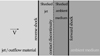 |
Fig. 1. Schematic diagram showing the formation of forward and reverse shocks in the termination region of YSO jets and novae outflows interacting with an ambient medium. The arrow indicates the fluid velocity direction in the laboratory frame. |
The jet density in the termination region can be calculated from conservation of mass as (Rodríguez-Kamenetzky et al. 2017)
 (1)
(1)
where Ṁi is the ionised mass loss rate and Rj is the radius of the section of the jet in the termination region.
In the strong shock approximation, the plasma is compressed by a factor of four and the temperature is Tps ∼ 2 × 10⁵(vsh/100 km s−1)2 K immediately after the shock front. Establishing the nature of the shocks, whether they are adiabatic or radiative, can be done by comparing the advection (escape) timescale tesc ∼ Rj/(vsh/4) to the cooling timescale
 (2)
(2)
where Λ(T) is the cooling function, which depends strongly on the temperature T. For the case of novae, which are characterised by high shock velocities and thus high temperatures, we use free-free emission which is given by  erg cm3 s−1. Shocks in YSO jets have lower velocities and therefore metal-line cooling dominates (e.g. Sutherland & Dopita 1993).
Equivalently, we can compare the (thermal) cooling length lcool = tcoolvsh/4 and Rj. The condition lcool > Rj (Heathcote et al. 1998) for a YSO shock to be adiabatic can be rewritten as vsh > vsh, ad, where
 (3)
(3)
In order to study the nature of the two shocks in the termination region, i.e. whether they are adiabatic or radiative, we sample the parameter space for nj and na for the cases of YSO jets and novae outflows presented in Table 1.
2.1. Young stellar objects
Stars are formed within dense molecular clouds, accreting matter onto the central protostar with the formation of a circumstellar disc and bipolar jets. These ejections are collimated flows of disc and stellar matter accelerated by magnetic field lines (Blandford & Payne 1982; Shu et al. 1994), and moving with speeds of vj ∼ 100 − 1000 km s−1 into the ambient molecular cloud. Molecular matter from the cloud is entrained by the jet, forming molecular outflows.
The ionised mass-loss rate in YSO jets is 10−8 ≤ Ṁi ≤ 10−5 >M⊙ yr−1, and the width of the jet in the termination region is characteristically Rj ∼ 1016 cm. By inserting these values into Eq. (1), we find nj in the range 1 − 103 cm−3. The ambient medium is the molecular cloud where the protostar is embedded, and typical values of na are in the range 10 − 105 cm−3. This results in values 10−5 ≤ χ ≤ 10. We consider vj = 300 and 1000 km s−1 and use the condition given by Eq. (3) to classify the shocks. The results are shown in Fig. 2.
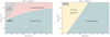 |
Fig. 2. Shock nature diagnostic in the termination region of a YSO jet for different jet and ambient densities, for vj = 300 (left) and 1000 km s−1 (right). The pink region indicates when the forward shock (FS) and the reverse shock (RS) are radiative, while the larger green region indicates when the forward shock is radiative and the reverse shock is adiabatic. Grey colour indicates an adiabatic forward shock and a radiative reverse shock while the yellow area shows when both shocks are adiabatic. The white dot indicates the parameters used in the numerical simulations in Sect. 4. |
Figure 2 indicates when the shocks are radiative or adiabatic, the left plot corresponds to vj = 300 km s−1 and the right plot to a faster jet with vj = 1000 km s−1. The particular case for na = 500 cm−3 and nj = 5 cm−3 for vj = 300 km s−1, marked with a white dot in the figure, is investigated in detail with 2D numerical simulations in Sect. 4. For faster YSO jets, vj = 1000 km s−1, the green region is larger, and in the range of densities studied here there is no region where both shocks are radiative (no pink region). We can conclude that for a large range of parameters for the ambient medium and the jet, we can expect the formation of the adiabatic–radiative shocks that are of particular interest in this work.
2.2. Classical novae
In order to study the shocks produced in classic novae, we follow the model of Metzger et al. (2015); see also Metzger et al. (2016). The shocks in novae outflows are formed from the collision of a slow shell ejection with velocity Vej ∼ 1000 km s−1, produced in the thermonuclear runaway, and a faster outflow or continuous wind of velocity Vw ∼ 2 Vej that follows the ejecta within a few days. The collision, as in the case of YSO jets, produces a system of two shocks: forward and reverse.
The forward shock propagates through the slow shell and the reverse shock moves back through the wind. The shock velocities depend on the density ratio of the colliding media. The expressions are the same as the ones presented at the beginning of this section with vj = Vw − Vej. The slow shell density is  , where Mej is the mass of the ejecta, Rej = Vejtej its expansion radius, and fΔΩ ∼ 0.5 is a filling factor related to the geometry of the model, i.e. the fraction of the total solid-angle subtended by the outflow. By considering typical values for the slow ejecta, we obtain
 (4)
(4)
The typical mass-loss rate of the fast wind is Ṁw = 10−5 M⊙ wk−1, giving a wind density for an outflow with radius Rej of
 (5)
(5)
(see Eq. (1)).
We study a parameter space for nej and nw varying between 10−5 ≤ Mej/M⊙ ≤ 10−2 and 10−6 ≤ Ṁw/M⊙ wk−1 ≤ 10−3. We consider Vej = 1000 km s−1 and 3000 km s−1. To classify the shocks we compare the cooling time given by Eq. (2) assuming free-free cooling and the typical duration of this phenomena of ∼2 weeks. The results are shown in Fig. 3.
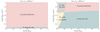 |
Fig. 3. Shock nature diagnostic in a nova forward–reverse system, with Vej = 1000 (left) and 3000 km s−1 (right). The colour coding is the same as in Fig. 2. |
In the case of a slow ejecta with Vej = 1000 km s−1, the forward shock is always radiative, and therefore the nature of the shock system is given by the reverse shock, which is radiative for Mej > 10−5.6 M⊙ (pink region on the left plot). The case of interest in this work, an adiabatic reverse shock with a radiative forward shock, corresponds to the smaller green region. In the case of a faster ejecta, Vej = 3000 km s−1, we obtain a similar plot to that in the case of YSO jets in Fig. 2. The area of the right plot in Fig. 3 is divided into: both adiabatic in the lower left (yellow), both radiative in the upper right (pink), an adiabatic forward shock and a radiative reverse shock in the top left (grey), and the opposite situation in the bottom right (green). In this case, the condition for a reverse shock to be adiabatic with an efficiently cooling forward shock is dominant in the given parameter space.
The very high densities in novae make the shocks very prone to efficient radiative cooling. However, we can conclude that under the model adopted, the possibility of having adiabatic shocks in these systems is plausible, especially for Vej > 1000 km s−1.
3. Instabilities at the contact discontinuity
The density of the plasma downstream of the radiative forward (bow) shock is
 (6)
(6)
(e.g. Blondin et al. 1990) when the plasma is cooled down to a temperature T, making the density contrast at the contact discontinuity  . As a consequence, the contact discontinuity is vulnerable to dynamical and thermal instabilities. A dense layer of density
  located at distance lth downstream of the bow shock fragments into several clumps (e.g. Calderón et al. 2020). However, we note that the component of the magnetic field in the ambient medium parallel to the bow shock front (Ba, ⊥) limits the compression factor to a maximum value of
 (7)
(7)
This indicates that significant enhancement in the plasma density downstream of the reverse shock is feasible if instabilities grow quickly enough to fragment the dense shell and form such clumps.
Rayleigh-Taylor instabilities
The Rayleigh-Taylor (RT) instability can grow in the contact discontinuity because of the velocity shear and the force exerted by the downstream material of the reverse shock on the forward shock.
If the forward shock is radiative, the formation of a shell much denser than nj and na at the contact discontinuity makes the working surface unstable even in the case of light jets. Following the analysis in Blondin et al. (1990), the acceleration of the dense shell with a width Wsh can be written as  .
.
The growth time of RT instabilities is  , where k is the wavenumber. By considering the characteristic dynamical timescale tdyn = 4 Rj/vj we obtain
 (8)
(8)
The condition tRT/tdyn < 1 leads to
 (9)
(9)
where we assume λ = 2π/k ∼ Wsh.
4. Numerical study
We performed 2D hydrodynamic simulations with the PLUTO code (Mignone et al. 2007) to illustrate the physical processes mentioned in the previous sections. We are interested in simulating the physics in the interaction between the incoming material, the shocked incoming material, the contact discontinuity, the target shocked material, and the target material. Therefore, we study the fluid collisions in a 2D rectangular box of size Lx × Ly, with Lx = 4 Rj and Ly = 8 Rj in a uniform Cartesian grid of resolution 1024 × 2048. Boundary conditions are periodic in the x-direction (horizontal) and outflow in the y-direction (vertical). The fluids are assumed to follow an ideal equation of state with an adiabatic index of γ = 5/3.
In the presence of cooling, we use the tabulated cooling function, which includes metal-line cooling from Schure et al. (2009); see Sect. 2. Calculations are performed using a HLLC solver with parabolic reconstruction. The time integration is performed using a Runge-Kutta 2 algorithm controlled by a Courant-Friedrichs-Lewy number of 0.4.
We simulate the case of a protostellar jet (Rj = 1016 cm) impinging upon an ambient molecular cloud. The results can be extrapolated to the case of novae. Initially, we have a fluid of density nj = 5 cm−3 and velocity vj = 300 km s−1
 at Tj = 1000 K for y ≤ 4 Rj colliding with a material at rest of density na = 500 cm−3 and temperature at Ta = 100 K for y > 4 Rj with na/nj = 100. According to our analytical estimates in Sect. 2, this configuration should develop a working surface composed of an adiabatic reverse shock and a radiative forward shock. The white dot in Fig. 2 shows the position of these parameters in the shock diagnostic map.
4.1. Results
Figure 4 shows the density (top) and temperature (bottom) profile of the system along the y-direction, averaged in x, for a time t = 0.04 tphy, where tphy ≡ Rj/105 cm s−1 = 1011 s is the physical time of the simulation. Both shocks are strong, producing a density jump of the order of 4. The jet and ambient shocked gases reach temperatures of 1.8 × 10⁶ and 1.8 × 10⁵ K, respectively. Using the post-shock temperature, we measure the shock velocities in the simulations ( km s−1), while calculating the displacement of the shock fronts as time evolves. The shock front cells are established with good accuracy by searching for the position of a strong gradient in the temperature profile. The velocity of the contact discontinuity is the fluid velocity of the shocked material, which is directly extracted from the simulation by measuring the velocities of the shocked jet and the shocked ambient material. The measured velocities of the shocks and the contact discontinuity are in very good agreement with the values predicted by the theory. Using the equations in Sect. 2 we find that vrs = −362.72 km s−1 and vbs = 36.27 km s−1. The contact discontinuity is expected to move with a velocity of vcd ≈ 3vbs/4 = 27.27 km s−1.
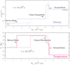 |
Fig. 4. Density (top) and temperature (bottom) profile along the vertical y-direction averaged in the horizontal x-direction for t = 4 × 10⁹ s. Dashed and solid lines correspond to the cases with and without cooling, respectively. |
In the presence of cooling, the system acts as predicted from theory: the shocked jet material experiences negligible cooling, while the shocked ambient material cools down. From the density (upper panel) and temperature (lower panel) plots in Fig. 4 (dashed lines), we see the typical profile of a radiative forward shock. The material behind the forward shock cools, i.e. the temperature drops, and compresses reaching values of  . Even when the radiative losses do not affect the reverse shock dynamics, a small drop in temperature can be seen, with Ts, cool/Ts ∼ 0.8. The cooling of the forward shock changes the contact discontinuity velocity (see the displacement of the contact discontinuity in Fig. 4 with respect to the case without cooling). This also slightly slows the reverse shock down, changing the shock Mach number M and hence the jump conditions across the shock (see e.g. Gintrand et al. 2021). The reverse shock velocity measured in the simulation with cooling is vrs ∼ −324 km s−1, giving Mcool ∼ 87.5; in the case without cooling M ∼ 98. The temperature jump condition can be written as Ts/T ∼ 5/16 M2 for a strong shock with γ = 5/3. Therefore,
  . A difference in the reverse post-shock density is not observed and also not expected because for strong shocks the density jump condition is practically independent of the shock Mach number.
The fluid profile propagates without disturbances in this simple configuration, without mixing of the jet and cloud materials. However, in a real situation the system will suffer perturbations produced by local inhomogeneities for example. In order to study the instabilities that might arise in the evolution of the system (see previous section), we consider a sinusoidal interface  , with y0 = 4 and L = 2 between the jet and cloud material, which mimics a perturbation1. Figure 5 shows a sequence of density maps as time evolves. Instabilities develop in the contact discontinuity as predicted by the theory, which induce mixing and turbulence. The instability also heats the shocked ambient material locally. The density structures in the unstable layer resemble the typical finger structures developed when the RT instability is operating.
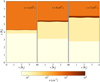 |
Fig. 5. Density maps for different evolving times. The interface is slightly perturbed (sinusoidal interface). |
In order to analyse the mixing of the two materials, we include a tracer field in the simulation that is advected with the fluid. Initially, the jet and ambient material have tracer values of 1 and 0, respectively. Figure 6 shows the tracer map at t = 7 × 10⁹ s zoomed into the forward shock region. The denser shocked ambient material penetrates the shocked jet material, and it is clear that mixing occurs as expected.
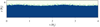 |
Fig. 6. Tracer map at t = 7 × 10⁹ s, zoomed at the forward shock region. The tracer indicates the advection of the jet and ambient materials as the system evolves. Initially the value of 1 is designated to the jet material (blue) and 0 to the ambient material (white). |
Magnetic field
In order to illustrate the effects of a magnetic field, we include a field Bj = 5 μG  and
and  in the MHD simulation setup. This gives a thermal-to-magnetic pressure ratio β of 0.7 for the jet, and 3.5 for the ambient medium. We also consider the case in which the magnetic field has no components perpendicular to Vsh (no
  -component). The ambient magnetic field component parallel to the shock front is compressed by the forward shock. Without cooling, the magnetic field compression is approximately 4, the same factor as the density. In the presence of cooling, further compression is expected and the field is amplified by a factor of about eight. The magnetic field map at t = 7 × 10⁹ s is shown in Fig. 7. The red arrows indicate the magnetic field direction in each cell plotted over the magnetic field intensity.
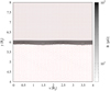 |
Fig. 7. Magnetic field intensity map at t = 7 × 10⁹ s. The red arrows show the magnetic field direction in the given grid point. |
The presence of a magnetic field inhibits or hinders the development of the instabilities discussed in Sect. 3. The effect of the magnetic field in the unstable layer can be seen in Fig. 8, where we show the density map zoomed into the forward shock region at t = 7 × 10⁹ s for hydrodynamic (top) and MHD (bottom) scenarios. Although the presence of the magnetic field reduces the development of instabilities and material mixing in the contact discontinuity, this effect is highly dependent on the magnetic field orientation. In the other case considered (only parallel B), the density structures developed by the instabilities exhibit a similar shape and level of material mixing as the non-magnetic case. In an actual astrophysical scenario, establishing the direction of the magnetic field is highly difficult and a number of assumptions are required.
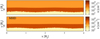 |
Fig. 8. Density maps zoomed into the forward shock region at t = 7 × 10⁹ s for the HD (top) and MHD (bottom) regimes. |
4.2. Power spectrum
We compute the power spectrum in the x direction for fixed height y at t = 7 × 10⁹ s. Figure 9 shows power spectra for the density (top) and the velocity (bottom) for two values of y. These heights correspond to different regions where density perturbations appear due to instabilities (see upper plot of Fig. 8). The mixing coefficient is defined as  , where kmax is the scale of the fastest growth rate of the unstable mode in the velocity. From Fig. 8 we estimate kmax ∼ 30 and
  . In physical units, this yields Dmix ∼ 2.4 × 1021 cm2 s−1. We can estimate the mixing time for a given size L0 by computing
 (10)
(10)
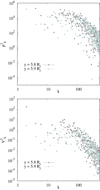 |
Fig. 9. Density (top) and velocity (bottom) power spectrum at t = 7 × 10⁹ s for two different heights. |
In the following section, we discuss the relevance of efficient mixing for enhancement of the gamma-ray emission by the interaction of relativistic particles with matter fields.
5. Gamma-ray emission
A system of two shocks, one radiative and the other adiabatic, can be present in YSO jets and novae outflows, as is demonstrated in Sect. 2. The fast reverse shock is more efficient for accelerating particles, as the acceleration time for electrons and protons with energy Ee and Ep, respectively, is
 (11)
(11)
in the Bohm diffusion regime. Furthermore, the adiabatic reverse shock has a luminosity
 (12)
(12)
which is higher than the forward radiative shock and can power the shock-accelerated population of particles. Also, the lower densities in the jet in the case of YSOs could avoid injection problems produced by ionisation and collision losses (e.g. O’C Drury et al. 1996).
Accelerated electrons and protons are injected into the shock downstream region with a luminosity Le, p = fLsh, where f ∼ 0.1 and 0.005 for the case of adiabatic and radiative shocks, respectively (Caprioli & Spitkovsky 2014). These particles must reach the contact discontinuity in order to interact with the cooled compressed layer. In the transport of the particles, various physical ingredients play a role. For simplicity, we only consider the spatial diffusion (energy dependent) and the advection by the large-scale gas velocity (energy independent). We only consider Bohm diffusion in the shock acceleration process, but far from the shock we expect a faster diffusion regime. Assuming a diffusion coefficient of D = 1025(Ee, p/10 GeV)0.5 cm2 s−1 (slower than the typical value in the ISM due to the instabilities) we obtain
 (13)
(13)
Advection downstream of the adiabatic shock over a distance Rj can be written as
 (14)
(14)
We define the residence time of particles in the downstream region as T = min{tadv, tdiff}.
The instabilities produced in the contact discontinuity (see e.g. Fig. 8) act to facilitate the interaction of particles with the denser, cool material. In addition, the mixing facilitates the transport and the collision of particles with denser material radiating more non-thermal emission via pp collisions (for hadrons) and relativistic Bremsstrahlung (for leptons). The timescale is very similar in both cooling processes. The simplest form of the relativistic Bremsstrahlung and pp cooling time reads
 (15)
(15)
We note that tBr, pp ∝ n−1 and therefore cooling through pp inelastic collisions and relativistic Bremsstrahlung becomes very efficient in the cooling layer where the density is significantly larger than 4nj.
The synchrotron cooling time of electrons in a magnetic field B is
 (16)
(16)
Inverse Compton (IC) scattering of IR and optical photons from the central object with luminosity L⋆ and energy density Uph = L⋆/(4πz2c) has a characteristic timescale of
 (17)
(17)
where z is the distance from the photon source.
5.1. Young stellar objects
Gamma-ray emission from YSO jets has been modelled in some recent papers (e.g. Araudo et al. 2021), but its detection has not been claimed to date. We show here that efficient mixing by RT instabilities in the contact discontinuity can significantly enhance the predicted gamma-ray emission levels, making them detectable in the GeV domain.
By considering B = 1 mG, Vsh ∼ 1000 km s−1, and a typical length scale of Rj ∼ 1016 cm, we plot in Fig. 10 the timescales of the processes mentioned above. We also plot tmix for comparison only, given that this value was not computed at the steady state. We can see that the acceleration is very efficient, together with the transport of particles by diffusion, giving a maximum energy of both electrons and protons of about 100 GeV. This transport ensures that the accelerated particles in the reverse shock reach the denser regions where materials start to mix and non-thermal emission is enhanced. On the contrary, the transport by advection drag the particles away downstream of the shocked jet material, which is subdominant in this case.
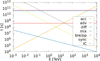 |
Fig. 10. Timescales as a function of energy for the interaction of high-energy particles for a YSO. |
Even though the real scenario might be much more complicated, these timescales indicate the dominating processes. However, we note that if the magnetic field is locally amplified by non-resonant hybrid instabilities, the maximum energy of protons will probably be determined by the available amplification time (Araudo et al. 2021). A detailed model is beyond the scope of the current study, but will be presented in a future work.
5.2. Novae
Gamma-ray emission has been detected from more than a dozen novae in the GeV range with most of the sources being classical novae (see Chomiuk et al. 2021, for a recent review). For example, Fermi and the High Energy Stereoscopic System (H.E.S.S.) recently detected high-energy and very-high-energy gamma-ray emission from the recurrent nova RS Ophiuchi (ATel#14834 and #14857, respectively); see further details below. The gamma-ray emission spans several orders of magnitude among the detected sources (Franckowiak et al. 2018). This difference might arise simply because the physical parameters are slightly different in each source. For example, we can see from the shock diagnostic maps in Fig. 3 that a change of a factor of three in velocity radically changes the possibilities of having adiabatic shocks in the system. Furthermore, changes in metallicity not considered here can modify the cooling function and might change the shock radiative efficiency.
A correlation between the optical and the gamma-ray emission has been claimed (e.g. Li et al. 2017; Aydi et al. 2020). This correlation appears to be strong in some systems but does not behave equally in all detected sources. In the systems where a correlation exists, it is highly probable that the emission is coming from the same spatial region, i.e. a radiative shock. However, this is not in conflict with our claims. Firstly, not all the possible physical parameters in novae result in adiabatic shocks and some sources might have an adiabatic–radiative shock combination. Secondly, even if the optical and gamma emission are coming from the same radiative shock, this does not confirm that the emitting non-thermal particles have been accelerated in that same shock. Indeed, the emission might arise when an underlying population of relativistic particles – accelerated in the reverse shock for example – is enhanced by the strong radiative shock compression (responsible for the optical emission) and even suffers reacceleration (e.g. Blandford & Cowie 1982). An interesting case that supports our findings is that of the nova V959 Mon (e.g. Fujikawa et al. 2012). This source has been detected as a GeV gamma-ray transient by Fermi (Ackermann et al. 2014). X-ray data analysis indicates that the reverse shock should be non-radiative (see, Nelson et al. 2021).
The hadronic scenario is one of the most favourable for explaining the high-energy radiation (e.g. Li et al. 2017; Martin et al. 2018). In this scenario, for protons to produce a gamma-ray of energy E through proton–proton collisions, they need to have energies of at least ten times E, which is not the case for electrons emitting through relativistic Bremsstrahlung. This last case favours the scenario of particles being accelerated at a reverse shock and radiating elsewhere, given that the most energetic particles diffuse more efficiently. A detailed modelling is needed to quantify the viability of the adiabatic–radiative shock scenario and this will be addressed in future works. Below we analyse the case of RS Oph, which was recently detected at gamma-rays.
The case of RS Oph
RS Oph is a symbiotic recurrent nova system that undergoes thermonuclear outbursts approximately every 20 years (e.g. Anupama 2008). The last detected optical outburst was during August 2021 (vsnet-alert 261312). The binary system, located at d = 1.6 kpc (Bode 1987), is composed of a white dwarf and a red giant (RG) companion (Dobrzycka & Kenyon 1994). Here we assume that in this source the shocks are produced in the collision of a fast wind with the dense and slow wind of the RG star (Vaytet et al. 2007, 2011). However, other models for RS Oph exist in the literature. In particular, given that the white dwarf in RS Oph is close to the Chandrasekhar limit, some authors modelled the system similarly to a supernova expanding in a wind medium (e.g. Walder et al. 2008; Booth et al. 2016).
The fast wind has an inferred velocity of Vw > 6000 km s−1 and a mass-loss rate of Ṁw ∼ 1.6 × 10⁻⁵ M⊙ yr−1 (Vaytet et al. 2011). The RG wind has a velocity of ∼15 km s−1 and ṀRG = 2 × 10⁻⁷ M⊙ yr−1. We assume a timescale of tej ∼ 2 weeks as in Sect. 2.2, and an orbital separation of a = 1.48 AU (e.g. Booth et al. 2016). For estimating the wind density nRG at a distance a, we use Eq. (5) properly normalised; we calculate the fast wind density as  . Using the expressions from Sect. 2, we obtain vbs ∼ 130 km s−1, vrs ∼ 5900 km s−1 for χ ∼ 5 × 10⁻⁴. We estimate tcool (see Eq. (2)) for the reverse shock, propagating through the fast wind, and the forward shock that develops in the RG wind in this case. We conclude that the reverse shock is highly adiabatic whereas the forward shock is highly radiative during tej.
The magnetic field strength near the reverse shock, B = 2 × 10⁻² G, is estimated assuming that the magnetic pressure is a fraction ϵB = 10−4 of the thermal pressure of the post-shock gas (see Metzger et al. 2015). The target radiation fields for IC in the vicinity of the reverse shock are the RG photon field URG at a distance of ∼a and the optical Uopt emission from reprocessed X-rays (Metzger et al. 2014). The companion star of the system is a M2III giant star (Zamanov et al. 2018), and we estimate a luminosity of LRG ∼ 2.5 × 1036 erg s−1 (see the adopted stellar parameter in Table 2). For estimating Lopt ∼ 7 × 1035 erg s−1, we assume that a small fraction, 10−2, of the shock power Lsh is radiated and reprocessed into optical emission.
Model and inferred parameters for RS Oph.
In Fig. 11 we show the relevant timescales involved in particle acceleration, diffusion, and radiation losses in the reverse adiabatic shock. Inverse Compton losses are very efficient, giving electrons maximum energies of ∼0.3 TeV. In the case of protons, the losses for pp do not affect the acceleration, which is limited only3 by the timescale of the event giving Ep, max ∼ 30 TeV. The diffusion of particles into the region of the contact discontinuity is fast, allowing the particles to further radiate there. The maximum energies of electrons and protons are compatible with high and very-high-energy gamma emission.
RS Oph was detected for the first time at gamma rays on August 2021 by Fermi Large Area Telescope (LAT) operating from 20 MeV to 300 GeV; the satellite detected a transient gamma-ray source positionally consistent with the nova. For its part, H.E.S.S., which operates in the energy range 10 GeV to 10 TeV, also detected a very-high-energy gamma-ray excess compatible with the direction of RS Oph. Following the detection, H.E.S.S. observations continued during the nova outburst. Here we show with a simple estimation that an adiabatic reverse shock is expected in RS Oph, and that it is capable of accelerating electrons and protons to high energies. The expected maximum energies are 0.3 TeV for electrons and 30 TeV for protons. In such dense environments, we expect significant pp emission up to 3 TeV. IC and Bremsstrahlung would be important at hundreds of GeV. Additional high-energy radiation, especially Bremsstrahlung and pp, is expected when particles diffuse to the contact discontinuity and compressed RG wind regions. The interaction of these high-energy particles can explain the detected gamma-ray emission. A detailed model of the system will be possible when observations become available.
6. MHD scaling of YSO jets and novae to laboratory experiments
In order to extend the scope of this work, we present preliminary estimates of the feasibility to scale the shocks from YSO jets and novae outflows to laboratory experiments. Laboratory experiments with dense, magnetised plasmas provide a novel approach to the study of astrophysical jets and outflows. The experiments are typically conducted on high-power laser and pulsed-power facilities (Remington et al. 2006), with each experimental approach allowing for different ranges of plasma parameters which can be chosen to match different regimes of interest. Typically, the experiments are characterised by temperatures of approximately hundreds to thousands of eV, flow velocities of approximately hundreds to thousands of km s−1, plasma volumes of ∼mm-cm3, timescales of approximately 1 to 100 ns, and electron densities of ≳1018 cm−3. The effect of magnetic fields can be controlled in the experiments depending on the way the plasma is driven in the experiment. In the case of pulsed-power generators, the magnetic field is produced from the strong electrical currents that drive the plasma, whereas in the case of laser experiments they can be generated from strong gradients of electron density and temperature in the plasma due to the Biermann battery effect, or introduced externally using capacitor-coil targets (Santos et al. 2018) or pulsed-power systems like MIFEDS (Fiksel et al. 2015).
MHD scaling arguments (e.g. Ryutov et al. 1999, 2000; Falize et al. 2011; Cross et al. 2014) make it possible to study astrophysical processes through laboratory experiments, for instance the launching and propagation of YSO jets (Lebedev et al. 2019) and accretion shocks (Van Box Som et al. 2017). Recently, the self-similar dynamics of the collision between adiabatic and radiative supersonic flows was studied by Gintrand et al. (2021), including an analysis of their scaling to laboratory experiments. Following the details given by Ryutov et al. (1999), the scaling is based on five characteristic physical parameters for the astrophysical and laboratory systems: length scale (R), density (n), pressure (P), velocity (v), and magnetic field (B). The ratio of length scales, density, and pressure result in three arbitrary scaling factors a, b, and c, which are further combined to constrain the timescale (t) and magnetic field.
The two systems will evolve identically if the initial conditions for the physical parameters are geometrically similar and the two dimensionless parameters, the Euler number Eu =  and thermal plasma beta β = 8πP/B2, are the same. The scaling will be valid if both systems have a fluid-like behaviour, i.e. a localisation parameter δ ≪ 1, and negligible dissipation processes, i.e. Reynolds (Re), Peclet (Pe), and magnetic Reynolds numbers (ReM) ≫ 1.
Table 3 summarises the MHD scaling for YSO jets and novae to a possible laboratory experiment. We fix the input astrophysical parameters (e.g. based on Table 1) and propose sensible laboratory parameters that match the scaling, resulting in scaling factors a = 1017 and b = c = 1018. For both YSO jets and novae, the laboratory parameters result in lengths scales of Rlab ∼ 1 mm, densities of nlab ∼ 1019 cm−3, pressures of Plab ∼ 105 bar, velocities of vlab ∼ 100 − 700 km s−1, magnetic fields of Blab ∼ 1 − 10 T, and timescales of tlab ∼ 1 ns. The temperature Tlab ∼ 1 keV was obtained under the assumption of astrophysical temperatures Tastro = 50 eV (5.8 × 10⁵ K) which is in line with those obtained in the simulations in Fig. 3. The dimensionless parameters in Table 3 fulfil the MHD scaling, with the exception of the Peclet number which for the laboratory case is ∼1.
MHD scaling of YSO jets and novae to laboratory experiments.
The parameters for scaled laboratory experiments are in line with plasma conditions achievable on current high-energy density facilities, such as the OMEGA laser at the University of Rochester, and future energetic, high-repetition lasers such as ELI-Beamlines in the Czech Republic (Jourdain et al. 2021).
7. Summary and conclusions
We study the interaction regions of YSO jets with an ambient medium and of classical novae outflows with previous ejected material. We show in Sect. 2 that for certain values of the jet or outflow and ambient densities, the working surface in both sources is composed of an adiabatic and a radiative shock. This particular system, in which the bow shock is radiative and the reverse shock is adiabatic, is very common in other astrophysical sources such as stellar bow shocks (e.g. del Valle & Pohl 2018). This shock combination is of interest for particle acceleration and subsequent non-thermal radiation. Particles are expected to be efficiently accelerated in strong adiabatic shocks, while the radiative shock produces a strong compression of the plasma (and magnetic field).
High-energy particles accelerated in the reverse adiabatic shock diffuse up to the dense layer downstream of the radiative shock where they can undergo further re-energisation by compression (e.g. Enßlin et al. 2011) and also an enhancement of radiative losses in the denser layer in the form of relativistic Bremsstrahlung for leptons and proton-proton inelastic collisions in the case of hadrons. We make order-of-magnitude estimates for the timescales and gamma-ray luminosity for the case of the YSO jet. In the case of novae, we model the source RS Oph recently detected for the first time in gamma rays. Our estimations indicate that the reverse shock is adiabatic and might accelerate particles up to high energies that could be responsible for the observed emission.
We find that the parameters for scaled laboratory experiments for YSO jets and nova outflows are in line with plasma conditions achievable in current high-power laser facilities. This provides new laboratory astrophysics working scenarios, especially in the case of novae outflows, which had never been explored with this approach before now.
In a real situation, perturbations are frequent, arising for example from density inhomogeneities, velocity gradients, and irregular geometry among other effects.
We do not consider any effect from the neutrals that might affect particle acceleration (see e.g. Metzger et al. 2016).
Acknowledgments
The authors thank the anonymous referee for carefully reading our manuscript and for her/his insightful comments and suggestions. M.V.d.V. is supported by the Grants 2019/05757-9 and 2020/08729-3, Fundação de Amparo à Pesquisa do Estado de São Paulo (FAPESP). A.T.A. thanks the Czech Science Foundation under the grant GAČR 20-19854S and the Marie Skłodowska-Curie fellowship. F.S.V. acknowledges the support from The Royal Society (UK) through a University Research Fellowship.
References
- Ackermann, M., Ajello, M., Albert, A., et al. 2014, Science, 345, 554 [NASA ADS] [CrossRef] [Google Scholar]
- Anupama, G. C. 2008, in RS Ophiuchi (2006) and the Recurrent Nova Phenomenon, eds. A. Evans, M. F. Bode, T. J. O’Brien, & M. J. Darnley, ASP Conf. Ser., 401, 31 [Google Scholar]
- Araudo, A. T., Padovani, M., & Marcowith, A. 2021, MNRAS, 504, 2405 [NASA ADS] [CrossRef] [Google Scholar]
- Aydi, E., Sokolovsky, K. V., Chomiuk, L., et al. 2020, Nat. Astron., 4, 776 [CrossRef] [Google Scholar]
- Blandford, R. D., & Cowie, L. L. 1982, ApJ, 260, 625 [NASA ADS] [CrossRef] [Google Scholar]
- Blandford, R. D., & Payne, D. G. 1982, MNRAS, 199, 883 [CrossRef] [Google Scholar]
- Blondin, J. M., Fryxell, B. A., & Konigl, A. 1990, ApJ, 360, 370 [NASA ADS] [CrossRef] [Google Scholar]
- Bode, M. F. 1987, RS Ophiuchi (1985) and the Recurrent Nova Phenomenon (Utrecht: VNU Science Press), 241 [Google Scholar]
- Booth, R. A., Mohamed, S., & Podsiadlowski, P. 2016, MNRAS, 457, 822 [NASA ADS] [CrossRef] [Google Scholar]
- Calderón, D., Cuadra, J., Schartmann, M., et al. 2020, MNRAS, 493, 447 [Google Scholar]
- Caprioli, D., & Spitkovsky, A. 2014, ApJ, 783, 91 [CrossRef] [Google Scholar]
- Carrasco-González, C., Rodríguez, L. F., Anglada, G., et al. 2010, Science, 330, 1209 [CrossRef] [Google Scholar]
- Chomiuk, L., Metzger, B. D., & Shen, K. J. 2021, ARA&A, 59, 48 [Google Scholar]
- Cross, J. E., Reville, B., & Gregori, G. 2014, ApJ, 795, 59 [NASA ADS] [CrossRef] [Google Scholar]
- de Gouveia Dal Pino, E. M. 2005, Adv. Space Res., 35, 908 [NASA ADS] [CrossRef] [Google Scholar]
- del Valle, M. V., & Pohl, M. 2018, ApJ, 864, 19 [NASA ADS] [CrossRef] [Google Scholar]
- Dobrzycka, D., & Kenyon, S. J. 1994, AJ, 108, 2259 [NASA ADS] [CrossRef] [Google Scholar]
- Doss, F. W., Kline, J. L., Flippo, K. A., et al. 2015, Phys. Plasmas, 22, 056303 [NASA ADS] [CrossRef] [Google Scholar]
- Enßlin, T., Pfrommer, C., Miniati, F., & Subramanian, K. 2011, A&A, 527, A99 [Google Scholar]
- Falize, É., Michaut, C., & Bouquet, S. 2011, ApJ, 730, 96 [NASA ADS] [CrossRef] [Google Scholar]
- Feeney-Johansson, A., Purser, S. J. D., Ray, T. P., et al. 2019, ApJ, 885, L7 [Google Scholar]
- Fiksel, G., Agliata, A., Barnak, D., et al. 2015, Rev. Sci. Instrum., 86, 016105 [NASA ADS] [CrossRef] [Google Scholar]
- Franckowiak, A., Jean, P., Wood, M., Cheung, C. C., & Buson, S. 2018, A&A, 609, A120 [NASA ADS] [CrossRef] [EDP Sciences] [Google Scholar]
- Fujikawa, S., Yamaoka, H., & Nakano, S. 2012, Cent. Bur. Electron. Telegr., 3202, 1 [Google Scholar]
- Gintrand, A., Moreno-Gelos, Q., Araudo, A., Tikhonchuk, V., & Weber, S. 2021, ApJ, 920, 113 [NASA ADS] [CrossRef] [Google Scholar]
- Hartigan, P. 1989, ApJ, 339, 987 [NASA ADS] [CrossRef] [Google Scholar]
- Heathcote, S., Reipurth, B., & Raga, A. C. 1998, AJ, 116, 1940 [Google Scholar]
- Jourdain, N., Chaulagain, U., Havlík, M., et al. 2021, Matter Rad. Extremes, 6, 015401 [CrossRef] [Google Scholar]
- Kuranz, C. C., Park, H. S., Huntington, C. M., et al. 2018, Nat. Commun., 9, 1564 [NASA ADS] [CrossRef] [Google Scholar]
- Lebedev, S. V., Frank, A., & Ryutov, D. D. 2019, Rev. Mod. Phys., 91, 025002 [NASA ADS] [CrossRef] [Google Scholar]
- Li, K.-L., Metzger, B. D., Chomiuk, L., et al. 2017, Nat. Astron., 1, 697 [Google Scholar]
- Livio, M. 1999, Phys. Rep., 311, 225 [NASA ADS] [CrossRef] [Google Scholar]
- Martin, P., Dubus, G., Jean, P., Tatischeff, V., & Dosne, C. 2018, A&A, 612, A38 [NASA ADS] [CrossRef] [EDP Sciences] [Google Scholar]
- Metzger, B. D., Hascoët, R., Vurm, I., et al. 2014, MNRAS, 442, 713 [NASA ADS] [CrossRef] [Google Scholar]
- Metzger, B. D., Finzell, T., Vurm, I., et al. 2015, MNRAS, 450, 2739 [Google Scholar]
- Metzger, B. D., Caprioli, D., Vurm, I., et al. 2016, MNRAS, 457, 1786 [NASA ADS] [CrossRef] [Google Scholar]
- Mignone, A., Bodo, G., Massaglia, S., et al. 2007, ApJS, 170, 228 [Google Scholar]
- Nelson, T., Mukai, K., Chomiuk, L., et al. 2021, MNRAS, 500, 2798 [Google Scholar]
- O’C Drury, L., Duffy, P., & Kirk, J. G. 1996, A&A, 309, 1002 [NASA ADS] [Google Scholar]
- Raga, A. C., Canto, J., & Cabrit, S. 1998, A&A, 332, 714 [NASA ADS] [Google Scholar]
- Remington, B. A., Drake, R. P., & Ryutov, D. D. 2006, Rev. Mod. Phys., 78, 755 [Google Scholar]
- Rodríguez-Kamenetzky, A., Carrasco-González, C., Araudo, A., et al. 2017, ApJ, 851, 16 [Google Scholar]
- Ryutov, D., Drake, R. P., Kane, J., et al. 1999, ApJ, 518, 821 [Google Scholar]
- Ryutov, D. D., Drake, R. P., & Remington, B. A. 2000, ApJS, 127, 465 [Google Scholar]
- Santos, J. J., Bailly-Grandvaux, M., Ehret, M., et al. 2018, Phys. Plasmas, 25, 056705 [NASA ADS] [CrossRef] [Google Scholar]
- Schure, K. M., Kosenko, D., Kaastra, J. S., Keppens, R., & Vink, J. 2009, A&A, 508, 751 [NASA ADS] [CrossRef] [EDP Sciences] [Google Scholar]
- Shu, F., Najita, J., Ostriker, E., et al. 1994, ApJ, 429, 781 [Google Scholar]
- Steinberg, E., & Metzger, B. D. 2018, MNRAS, 479, 687 [NASA ADS] [Google Scholar]
- Sutherland, R. S., & Dopita, M. A. 1993, ApJS, 88, 253 [Google Scholar]
- Suzuki-Vidal, F., Lebedev, S. V., Ciardi, A., et al. 2015, ApJ, 815, 96 [NASA ADS] [CrossRef] [Google Scholar]
- Van Box Som, L., Falize, E., Bonnet-Bidaud, J.-M., et al. 2017, MNRAS, 473, 3158 [Google Scholar]
- Vaytet, N. M. H., O’Brien, T. J., & Bode, M. F. 2007, ApJ, 665, 654 [NASA ADS] [CrossRef] [Google Scholar]
- Vaytet, N. M. H., O’Brien, T. J., Page, K. L., et al. 2011, ApJ, 740, 5 [NASA ADS] [CrossRef] [Google Scholar]
- Vlasov, A., Vurm, I., & Metzger, B. D. 2016, MNRAS, 463, 394 [NASA ADS] [CrossRef] [Google Scholar]
- Walder, R., Folini, D., & Shore, S. N. 2008, A&A, 484, L9 [NASA ADS] [CrossRef] [EDP Sciences] [Google Scholar]
- Zamanov, R. K., Boeva, S., Latev, G. Y., et al. 2018, MNRAS, 480, 1363 [NASA ADS] [CrossRef] [Google Scholar]
All Tables
All Figures
|
Fig. 1. Schematic diagram showing the formation of forward and reverse shocks in the termination region of YSO jets and novae outflows interacting with an ambient medium. The arrow indicates the fluid velocity direction in the laboratory frame. |
| In the text | |
|
Fig. 2. Shock nature diagnostic in the termination region of a YSO jet for different jet and ambient densities, for vj = 300 (left) and 1000 km s−1 (right). The pink region indicates when the forward shock (FS) and the reverse shock (RS) are radiative, while the larger green region indicates when the forward shock is radiative and the reverse shock is adiabatic. Grey colour indicates an adiabatic forward shock and a radiative reverse shock while the yellow area shows when both shocks are adiabatic. The white dot indicates the parameters used in the numerical simulations in Sect. 4. |
| In the text | |
|
Fig. 3. Shock nature diagnostic in a nova forward–reverse system, with Vej = 1000 (left) and 3000 km s−1 (right). The colour coding is the same as in Fig. 2. |
| In the text | |
|
Fig. 4. Density (top) and temperature (bottom) profile along the vertical y-direction averaged in the horizontal x-direction for t = 4 × 10⁹ s. Dashed and solid lines correspond to the cases with and without cooling, respectively. |
| In the text | |
|
Fig. 5. Density maps for different evolving times. The interface is slightly perturbed (sinusoidal interface). |
| In the text | |
|
Fig. 6. Tracer map at t = 7 × 10⁹ s, zoomed at the forward shock region. The tracer indicates the advection of the jet and ambient materials as the system evolves. Initially the value of 1 is designated to the jet material (blue) and 0 to the ambient material (white). |
| In the text | |
|
Fig. 7. Magnetic field intensity map at t = 7 × 10⁹ s. The red arrows show the magnetic field direction in the given grid point. |
| In the text | |
|
Fig. 8. Density maps zoomed into the forward shock region at t = 7 × 10⁹ s for the HD (top) and MHD (bottom) regimes. |
| In the text | |
|
Fig. 9. Density (top) and velocity (bottom) power spectrum at t = 7 × 10⁹ s for two different heights. |
| In the text | |
|
Fig. 10. Timescales as a function of energy for the interaction of high-energy particles for a YSO. |
| In the text | |
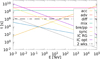 |
Fig. 11. As in Fig. 10 but for the nova RS Oph. |
| In the text | |
Current usage metrics show cumulative count of Article Views (full-text article views including HTML views, PDF and ePub downloads, according to the available data) and Abstracts Views on Vision4Press platform.
Data correspond to usage on the plateform after 2015. The current usage metrics is available 48-96 hours after online publication and is updated daily on week days.
Initial download of the metrics may take a while.