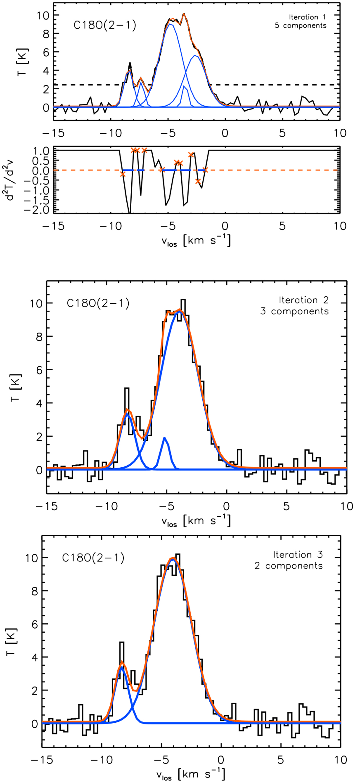
Example of an observed spectrum and the different steps of the n-Gaussian fitting procedure. Top: Observed C¹⁸O(2–1) spectra toward a position in the center of the map (top). The blue and red curves show the five individual Gaussian functions and the sum of all the fitted Gaussians, respectively. The dotted line shows the intensity threshold corresponding to S/N = 4s. Here s = 0.6 K. The second derivative of the C¹⁸O(2–1) spectra shown in the top panel (bottom). The blue horizontal lines show the region where the first guess for each of the Gaussian fits is identified indicated by the red symbols defining the points surrounding a peak to be fitted. Middle: Second iteration of the Gaussian fits where the Gaussian component not following the given criterion on the velocity resolution (5 × 0.3 km s^-1) are discarded. A new multi-component fit is done on the remaining positions. The result is a combined Gaussian with three components. Bottom: Third iteration of the Gaussian fits following the same procedure of the second iteration. The result is a combined Gaussian with two components. Both components follow the defined criteria and correspond to the final result of the n-Gaussian fit.