| Issue |
A&A
Volume 659, March 2022
|
|
|---|---|---|
| Article Number | A53 | |
| Number of page(s) | 6 | |
| Section | Stellar structure and evolution | |
| DOI | https://doi.org/10.1051/0004-6361/202142666 | |
| Published online | 04 March 2022 | |
Local heating due to convective overshooting and the solar modelling problem
1
University of Exeter, Physics and Astronomy, EX4 4QL Exeter, UK
e-mail: This email address is being protected from spambots. You need JavaScript enabled to view it.
2
École Normale Supérieure, Lyon, CRAL (UMR CNRS 5574), Université de Lyon, France
3
Department of Physics and Astronomy, Georgia State University, Atlanta, GA 30303, USA
4
Centre for Fusion, Space and Astrophysics, Department of Physics, University of Warwick, Coventry CV4 7AL, UK
Received:
15
November
2021
Accepted:
22
December
2021
Abstract
Recent hydrodynamical simulations of convection in a solar-like model suggest that penetrative convective flows at the boundary of the convective envelope modify the thermal background in the overshooting layer. Based on these results, we implement in one-dimensional stellar evolution codes a simple prescription to modify the temperature gradient below the convective boundary of a solar model. This simple prescription qualitatively reproduces the behaviour found in the hydrodynamical simulations, namely a local heating and smoothing of the temperature gradient below the convective boundary. We show that introducing local heating in the overshooting layer can reduce the sound-speed discrepancy usually reported between solar models and the structure of the Sun inferred from helioseismology. It also affects key quantities in the convective envelope, such as the density, the entropy, and the speed of sound. These effects could help reduce the discrepancies between solar models and observed constraints based on seismic inversions of the Ledoux discriminant. Since mixing due to overshooting and local heating are the result of the same convective penetration process, the goal of this work is to invite solar modellers to consider both processes for a more consistent approach.
Key words: stars: evolution / stars: interiors / Sun: helioseismology / Sun: interior / convection
© ESO 2022
1. Introduction
Modelling the internal structure of the Sun is still a challenge. A recent review by Christensen-Dalsgaard (2021) describes in detail the long-standing efforts to improve solar models. The solar modelling problem refers to the discrepancy between helioseismology and solar interior models that adopt low metallicities predicted by the three-dimensional (3D) atmosphere models of, for example, Asplund et al. (2009) and Caffau et al. (2011), in contrast to the high metallicities based on previous literature compilations by, for example, Anders & Grevesse (1989) and Grevesse & Noels (1993). Asplund et al. (2021) have recently confirmed with state-of-the-art 3D simulations the relatively low metal abundances for the Sun. Asplund et al. (2021) consider that their study yields the most reliable solar abundances available today, suggesting that the solar modelling problem is no longer a problem of abundances but rather a problem of stellar physics. The treatment of mixing below the convective zone is one of the key processes that could improve solar models. Several studies indeed reveal that the process of convective penetration, also called overshooting, at the bottom of the convective envelope could play an important role in improving the agreement between solar models and helioseismic constraints (see for example Christensen-Dalsgaard et al. 2011; Zhang et al. 2012; Buldgen et al. 2019a). Overshooting in solar models has most often been treated using diffusive or instantaneous chemical mixing. A temperature gradient that sharply transitions from a nearly adiabatic form to a radiative form is usually assumed, as suggested by the theoretical work of Zahn (1991). Models with a smoother transition have also been investigated. Based on the analysis of models with different stratifications near the base of the convective zone, Christensen-Dalsgaard et al. (2011) found that models that better fit the helioseismic data have a weakly sub-adiabatic temperature gradient in the lower part of the convective zone and a smooth transition to the radiative gradient in the overshooting layer. But Christensen-Dalsgaard et al. (2011) noted that the required temperature stratification is difficult to reconcile with existing overshooting models and numerical simulations. They concluded that only non-local turbulent convection models could produce the desired degree of smoothness in the transition (see for example Zhang & Li 2012; Zhang et al. 2012). But these non-local models remain uncertain, and their description of overshooting under the conditions found at the base of the solar convective zone is yet to be validated. Zhang et al. (2019) explored the impact of overshooting by introducing a parametrised turbulent kinetic energy flux based on a model with parameters that are adjusted to improve the helioseismic properties. They suggest that amelioration can be obtained specifically below the convective envelope. However, Zhang et al. (2019) find that this model cannot solve the whole solar problem because such a flux worsens the sound-speed profile in the deep radiative interior of their solar model. Given the uncertainties regarding the temperature stratification of the overshooting region, solar modellers have considered these effects as secondary and have focused their efforts on exploring the impact of solar abundances, microphysics (opacities, equations of state, nuclear reaction rates), and chemical mixing and diffusion (see details and references in the review of Buldgen et al. 2019b). Additional, more exotic effects such as early disk accretion or solar-wind mass loss (Zhang et al. 2019; Kunitomo & Guillot 2021) are also attracting increasing attention.
To reinvigorate the debate, Buldgen et al. (2019a) recently highlighted once again how the transition of the temperature gradient just below the convective envelope can significantly impact the disagreement between solar models and helioseismic constraints. Their results, based on a method that combines multiple structural inversions, suggest that the transition in temperature gradient is improperly reproduced by adopting either an adiabatic or a radiative temperature gradient in the overshooting layer. The solution should be somewhere in between these two extremes. Christensen-Dalsgaard et al. (2018) also note that an increase in the temperature at the transition would remove a remaining small sharp dip in the speed of sound immediately beneath the convective zone of the model. A major difficulty is to disentangle the effects of overshoot from the effects of opacities, which can also alter the temperature gradient in these layers. Given the large number of parameters to deal with in order to improve solar models and the current lack of strong arguments in favour of modifying the thermal stratification in the overshooting layer, there has been no real motivation to deviate from the traditional picture of a sharp transition as formalised by Zahn (1991).
The present work is motivated by arguments inspired by hydrodynamical simulations of convection and convective penetration in solar-like models. Recent hydrodynamical simulations by Baraffe et al. (2021, hereafter B21) highlight the process of local heating in the overshooting region due to penetrating convective motions across the convective boundary. In the following, we analyse the potential impact of this feature on one-dimensional (1D) stellar evolution structures in the context of solar models. The hydrodynamical results of B21 are briefly summarised in Sect. 2, and their impact on 1D models are analysed in Sect. 3 and discussed in Sect. 4.
2. Modification of the thermal background in the overshooting layer: Results from two-dimensional hydrodynamical simulations
B21 performed two-dimensional (2D) fully compressible time-implicit simulations of convection and convective penetration in a solar-like model with the MUlti-dimensional Stellar Implicit Code MUSIC (Viallet et al. 2011, 2016; Goffrey et al. 2017). The main motivation was to explore the impact of an artificial increase in the stellar luminosity on the properties of convection and convective penetration. This procedure is a common tactic adopted in hydrodynamical simulations of convection (Rogers et al. 2006; Meakin & Arnett 2007; Brun et al. 2011; Hotta 2017; Edelmann et al. 2019). The experiments of B21 highlight the impact of penetrative downflows on the local thermal background in the overshooting layer. They illustrate how convective downflows, when penetrating the region below the convective boundary of the envelope, can induce a local heating and a modification of the temperature gradient as a result of compression and shear in the overshooting layer. This modification of the local background is connected to a local increase in the radiative flux to counterbalance the negative enthalpy flux (or heat flux) produced by penetrating flows. The negative peak of the enthalpy flux and the positive bump of the radiative flux below the convective boundary are well-known features described in many numerical works (Hurlburt et al. 1986; Muthsam et al. 1995; Brummell et al. 2002; Brun et al. 2011; Hotta 2017; Käpylä 2019; Cai 2020). A few works (Rogers et al. 2006; Viallet et al. 2013; Korre et al. 2019; Higl et al. 2021) have also reported a modification of the local thermal background in the overshooting region, but without providing a detailed description. The simulations of B21 provide a physical explanation that links the convective penetration process to the local heating and to the radiative bump in the overshooting layer. The solar-like star simulated in B21 is based on a model that is not thermally relaxed. It is reasonable to assume that the local heating seen in B21 is present in stars because the negative heat flux in the overshooting layer and the bump in the radiative flux that compensates for this feature are persistent. These two features are also commonly observed in other hydrodynamical simulations, as mentioned above. An exploration of the impact of this heating on stellar evolution models may reveal that heating is a necessary aspect of models for overshooting.
The behaviour of the thermal profile below the convective boundary found in the simulations of B21 is illustrated in Fig. 1. It is displayed for the model with a realistic stellar luminosity (lower panel). We also show the results for a model with an artificial enhancement in the luminosity by a factor of ten because the features are intensified in these ‘boosted’ models (upper panel). The figure shows the local heating in the overshooting layer and its impact on the sub-adiabaticity (∇−∇ad), with  the temperature gradient and
  the adiabatic gradient. The initial stratification below the convective boundary (located at r = 0.6734 × Rstar for this specific stellar model) is set by the stable radiative gradient, ∇rad (see the dashed black line below the convective boundary in Fig. 1). B21 show that, as a result of the local heating below the convective boundary characterised by the bump in temperature difference ΔT/T0 displayed in Fig. 1, the temperature gradient becomes less sub-adiabatic immediately below the convective boundary1. The net result is a smoother transition just below the convective boundary with a temperature gradient that has an intermediate value between the radiative temperature gradient and the adiabatic one. In the next section we analyse the impact of this local heating on 1D solar structures by adopting a simple prescription that mimics the behaviour of the temperature gradient suggested by hydrodynamical simulations.
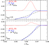 |
Fig. 1. Radial profile of the temperature departure ΔT/T0 from the initial profile T0 and of the sub-adiabaticity (∇−∇ad) close to the convective boundary predicted by 2D hydrodynamical simulations (B21) of solar-like models. Lower panel: model with a realistic stellar luminosity and upper panel: model with luminosity enhanced by a factor of ten. The dash-dotted red lines show ΔT/T0 (in %), the relative difference between the time and space averages of the temperature, T, and the initial temperature, T0. The solid blue lines show the time and space averages of the sub-adiabaticity (∇−∇ad). The dashed black lines show the initial profile of the sub-adiabaticity, (∇−∇ad)init. The convective boundary is indicated by the vertical solid line (see details in B21). |
3. Impact on one-dimensional solar structure models
3.1. Helioseismic constraints
Our primary goal in this short paper is to illustrate the potential, qualitative impact of the local heating produced by overshooting. We adopted a strategy inspired by the analysis of Buldgen et al. (2020), who constructed a static structure of the Sun in agreement with seismic inversions of the Ledoux discriminant defined by
 (1)
(1)
with Γ1 = (∂lnP/∂lnρ)ad. Starting from a reference evolutionary model, Buldgen et al. (2020) used an inversion procedure to iteratively reconstruct a solar model. Successive inversions of the Ledoux discriminant allowed them to obtain a model-independent profile for this quantity. Their reconstruction method also gives solar structures that are in excellent agreement with other structural inversions, namely the entropy, S, the square of the speed of sound,  , and the density, ρ. To illustrate the convergence of their reconstruction procedure, they show (right panels of their Figs. 3–6) the successive iterations that converge to an excellent level of agreement for the four structural inversions (A, S,
  , ρ) starting from the initial reference model adopted in their work. The differences found between the reconstructed model and the reference model are useful as they indicate the modifications of the reference model that are required to converge towards a solar model in agreement with helioseismic data. We recall here the major trends found by Buldgen et al. (2020) for the four structural quantities, which are used for our analysis in Sect. 3.2.
The first concerns the Ledoux discriminant. The major discrepancy between the Sun and the reference model occurs just below the convective boundary, with a large positive bump for the quantity (ASun − Aref).
The second concerns the speed of sound. The same positive bump at the same location as for the Ledoux discriminant, A, is observed for the quantity  . The corrections applied to A during the reconstruction procedure also reduce the discrepancy in the speed of sound in the radiative region.
The third concerns the entropy. Large discrepancies are observed in both the radiative region and the convective zone. The entropy discrepancy (SSun − Sref)/Sref has two positive peaks in the radiative zone, one just below the overshooting region and a larger peak deeper at ∼40% of the stellar radius. This discrepancy is negative in the convective zone. The corrections applied to A help reduce these entropy discrepancies in both regions.
The fourth concerns the density. The quantity (ρSun − ρref)/ρref has a negative peak in the radiative region, at ∼ 35% of the stellar radius, and is positive in the convective zone.
Importantly, Buldgen et al. (2020) mention that their reconstruction procedure gives similar Ledoux discriminant profiles for a wide range of initial reference models. We used these results to gauge whether the modifications of the thermal profile predicted by B21 can help in qualitatively improving all the structural quantities used by Buldgen et al. (2020).
3.2. Testing one-dimensional solar models
Our main motivation is to show the potential impact of the local heating described in Sect. 2 on stellar models. We are not aiming in this short work at constructing the best solar model to fit helioseismic constraints. Using stellar evolution codes, we have adopted two different methods that can be found in the literature to construct solar models (e.g. Zhang et al. 2012; Vinyoles et al. 2017). Our first method relies on the thermal relaxation of a reference model with solar radius and luminosity that is modified to reproduce the temperature gradient in the overshooting layer suggested by hydrodynamical simulations. In this case, the chemical abundances are not modified by nuclear reactions, mixing, or microscopic diffusion during the relaxation process. For these tests, we used the 1D Lyon stellar evolution code (Baraffe et al. 1998). We repeated this experiment based on thermal relaxation with the stellar evolution code MONSTAR (e.g. Constantino et al. 2014) and obtained the same qualitative results.
The second method considers models that account for the modification of the temperature gradient in the overshooting layer from the zero age main sequence (ZAMS). The models are then evolved until they reach the solar radius and luminosity. With this approach, changes in the chemical abundances from nuclear reactions, microscopic diffusion, and overshooting mixing are also consistent with any modification of the structure induced by the forced local heating in the overshooting layer. These tests were performed with MONSTAR as it includes the treatment of microscopic diffusion.
The first method allows the impact of local heating in the overshooting layer after thermal relaxation to be isolated. The second method provides evolutionary models that are self-consistent since the effect of the modification of the temperature gradient is accounted for during their evolution on the main sequence.
In the following, we adopt a modification of the local temperature gradient in the overshooting layer that qualitatively reproduces the behaviour displayed in Fig. 1. We define an overshooting length dov = αovHP, CB, with HP, CB the pressure scale height at the convective boundary and αov a free parameter. We also define two radial locations, rov = rCB − dov and rmid = rCB − dov/2, with rCB the radial location of the convective boundary. The temperature gradient is modified as follows. For rmid ≤ r < rCB, we use
 (2)
(2)
with
![Mathematical equation: $$ \begin{aligned} g(r)=\mathrm{sin}\{ [(r - r_{\rm mid})/(r_{\rm CB} - r_{\rm mid})]^a \times \pi /2\}. \end{aligned} $$](/articles/aa/full_html/2022/03/aa42666-21/aa42666-21-eq8.gif) (3)
(3)
For rov ≤ r < rmid, we use
 (4)
(4)
with
![Mathematical equation: $$ \begin{aligned} h(r)=b \times sin\{ [(r_{\rm mid} -r)/(r_{\rm mid} - r_{\rm ov}) ] \times \pi \}. \end{aligned} $$](/articles/aa/full_html/2022/03/aa42666-21/aa42666-21-eq10.gif) (5)
(5)
Sine functions are used in Eqs. (3) and (5) to reproduce the smooth variations in the temperature gradient below the convective boundary produced by the hydrodynamical simulations. We have verified that the results are insensitive to the smoothness of these variations and to the exact shape of the temperature gradient radial profile. We adopted a = 0.3 in Eq. (3) as it provides a behaviour for the temperature gradient very close to the one displayed in Fig. 1. Results are rather insensitive to variations in the values of a between 0.2 and 0.4. We adopted b = 0.03 in Eq. (5), which also provides a close visual match to the hydrodynamical results, but we note that the results are insensitive to the value of b.
3.2.1. Thermal equilibrium models
The details of the procedure for the first method are the following. We calculate the evolution of a 1 M⊙ model with an initial helium mass fraction of 0.28, metallicity Z = 0.02, and a mixing length lmix = 1.9HP. We use a reference model that is in thermal equilibrium2 and has the luminosity and radius of the current Sun. Starting from this reference model, the temperature gradient is modified over a prescribed depth to mimic the impact of overshooting according to the hydrodynamical simulations described in Sect. 2. We adopt the prescription given by Eqs. (2)–(5) over a distance dov below the convective boundary. We show the results in Fig. 2 for αov = 0.15 and αov = 0.20. These overshooting widths are in good agreement with the maximal depth reached by downflows below the convective boundary predicted by the hydrodynamical simulations for the solar-like model investigated in B21. We note that the stellar model used in B21 is slightly under-luminous compared to the Sun (see B21 for details). B21 also mention that one should be cautious when directly applying the overshooting depths predicted by their simulations to real stars since the final relaxed state for these simulations may have different properties from non-thermally relaxed states. We varied αov between 0.15 and 0.35 and find that the results do not change qualitatively. However, the amplitude of the variations in the model properties depends on dov (see below). As shown below, this simple prescription implemented in a stellar evolution code yields a local increase in the temperature below the convective boundary, similar to that observed in the hydrodynamical simulations. We stress that Eqs. (2)–(5) have been chosen for simplicity. They are only a rough approximation that can mimic the thermal profile behaviour suggested in the 2D simulations.
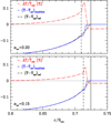 |
Fig. 2. Radial profile of the temperature difference and of the sub-adiabaticity of a 1D solar-like structure with a modified temperature gradient in the overshooting layer according to Eqs. (2)–(5). The temperature gradient is modified over a distance dov = αovHP, CB, with αov = 0.15 in the lower panel and αov = 0.20 in the upper panel. The dash-dotted red lines show the percentage relative temperature difference, ΔT/Tref, with ΔT = T − Tref. The solid blue lines correspond to the sub-adiabaticity (∇−∇ad). The dashed black lines show the sub-adiabaticity of the reference model. The convective boundary is indicated by the vertical solid line. The vertical dashed line in each panel is located at a distance dov below the convective boundary. |
The model with a modified temperature gradient is then thermally relaxed, that is to say, it is evolved over many thermal timescales without any modification of the abundances from nuclear reactions until thermal equilibrium is reached. The temperature gradient is modified in the overshooting layer during the whole relaxation process, and this is referred to as a ‘forced local heating’. This procedure ensures that the model with a modified temperature gradient can be consistently compared to the reference model. As shown in Fig. 2, the simple prescription given by Eqs. (2)–(5) yields similar qualitative changes in the temperature and the sub-adiabaticity close to the convective boundary that was found in the hydrodynamical simulations of B21.
The impact on the whole stellar structure was quantified by comparing the four structural quantities (A, S,  , ρ) between the modified and the reference model. The results are displayed in Fig. 3, with ΔX defined as (X − Xref) for any structural quantity X. The forced local heating in the overshooting layer produces similar positive peaks for ΔA, ΔS, and
  , as found for the temperature. The modification thus provides the correction required to improve the discrepancy for the Ledoux discriminant described in the first of the trends outlined in Sect. 3.1. Unsurprisingly, such a modification of the temperature gradient is expected to improve the agreement with helioseismic constraints and help remove the sound speed anomaly below the convective boundary (second trend in Sect. 3.1), as suggested by the results of Christensen-Dalsgaard et al. (2011). But it is also interesting to note that such a modification yields a slight cooling of the convective zone (see Fig. 2) and thus a negative difference for the entropy (see Fig. 3). A negative difference in the convective envelope is in agreement with the correction required for the reference model of Buldgen et al. (2020) to better match the Sun (see third trend in Sect. 3.1). Regarding the density, the modification of the temperature gradient has an interesting impact in the radiative zone, with a large decrease in the density compared to the reference model over a broad region below the convective boundary. The impact on the density in the convective region for this specific model is partly in agreement with the correction required for this quantity in the Buldgen et al. (2020) study, with a positive difference found only in the upper part of the convective envelope (see the fourth trend in Sect. 3.1).
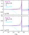 |
Fig. 3. Difference of various structural quantities between a model with a modified temperature gradient in the overshooting layer and a reference model calculated with the Lyon stellar evolution code. The temperature gradient in the modified model is changed over a distance dov = αovHP, CB below the convective boundary (indicated by the vertical solid line). Lower panel: results for αov = 0.15 and upper panel: for αov = 0.20. |
These trends are insensitive to the depth over which the temperature gradient is modified. Increasing the depth increases the magnitude of the differences but has no impact on their sign. We find that the maximum variation in the model properties, such as the speed of sound,  , roughly scales with
  . This scaling is linked to the integrated area between the modified temperature gradient curve and the one for the reference (non-modified) temperature gradient, which roughly decreases linearly with r. This area is proportional to the square of the overshooting depth, and consequently, the maximum variation in the model properties is also proportional to
  . The qualitative trends also remain the same whether overshooting mixing in the reference model is ignored or included using a step function (with instantaneous mixing) or an exponential decay for the diffusion coefficient (e.g. Freytag et al. 1996).
3.2.2. Self-consistent evolutionary models
For the tests based on the second method, we ran different sets of models with different combinations of assumptions, including or not microscopic diffusion and with or without overshooting mixing. When overshooting mixing was included in the overshooting layer, it was based either on a step function or on an exponential decay for the diffusion coefficient. Microscopic diffusion for H and He was implemented according to Thoul et al. (1994). For these tests, the temperature gradient was modified according to Eqs. (2)–(5). All models start from the ZAMS and are evolved until they reach the solar radius and luminosity at the same age. This was achieved by making small adjustments to the mixing length, lmix. The models with temperature gradient modifications were compared to the relevant reference model, which has no modification of the temperature gradient but everything else is the same (i.e. the same treatment of microscopic diffusion and of overshooting mixing). The evolutionary models with temperature gradient modifications are thus self-consistent. The main difference between this approach and the one in the previous section is that these models accumulate small differences in, for example, central H abundance when compared to their reference model. These tests produce the same trends in the overshooting layer as found for the tests based on the first method (Sect. 3.2.1), independently of the treatment of overshooting mixing and whether microscopic diffusion is included or not. In the convective zone, all models give a positive difference for the density between the model with a modified temperature gradient and the relevant reference model. For the other quantities (S,  ), the differences in the convective zone are very sensitive to the assumptions regarding whether overshooting mixing is included or not. But at least we find solutions that are compatible with the four trends found by Buldgen et al. (2020) for the four structural quantities. This is illustrated in Fig. 4 with a model that accounts for step function overshooting mixing over a distance dov = 0.15HP, CB (lower panel) and dov = 0.20HP, CB (upper panel).
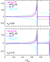 |
Fig. 4. Difference of various structural quantities between a modified model and a reference model calculated with the MONSTAR stellar evolution code. The reference model is evolved from the ZAMS with microscopic diffusion and step function overshooting mixing over a distance dov = αovHP, CB below the convective boundary. Lower panel: results for αov = 0.15 and upper panel: for αov = 0.20. The models with a modified temperature gradient in the overshooting layer (same microscopic diffusion and overshooting mixing treatment as the reference model) are evolved similarly from the ZAMS. The convective boundary is indicated by the vertical solid line. |
4. Conclusion
The tests performed in Sect. 3 are based on different methods (relaxed models versus consistent evolution) that can be used to construct solar models. Independently of the method used, the tests show that a local increase in the temperature in the overshooting region due to convective penetration provides the qualitative effects required to improve the speed of sound discrepancy below the convective boundary. This discrepancy is persistent in solar models that use low solar metal abundances. This is not surprising because an increase in the temperature in this specific region has previously been invoked in the literature to solve this problem, as mentioned in Sect. 1. However, the details of the physical process responsible for this local heating have been lacking, whereas we can now suggest an explanation based on the B21 results. The trends that we find for the four structural quantities (A, S,  , ρ) are robust below the convective boundary and in a large fraction of the radiative core, independently of the treatment of mixing and diffusion and of the method for constructing the models in Sects. 3.2.1 and 3.2.2. Our experiments additionally show that such a local change in the temperature, despite being made over a very limited region below the convective boundary, can also affect the density, the entropy, and the speed of sound in the convective envelope after thermal relaxation or evolution on the main sequence. How these quantities are affected in the convective envelope compared to a reference model with no local heating depends on the strategy for building solar models and on the treatment of overshooting mixing. This mixing is obviously linked to the local heating given that both result from the same dynamical process. A combined testing of both effects in stellar models could provide more constraints on the general process of overshooting.
Increasingly, efforts are now devoted to characterising the process of convective boundary mixing in stellar models based on multi-dimensional hydrodynamical simulations. More work is required to obtain reliable determinations of an overshooting depth and to describe quantitatively the mixing and impact on the temperature gradient. Understanding the effects of rotation and magnetic fields on overshooting is a significantly more difficult theoretical and numerical problem to address; however, efforts to study these combined non-linear effects are ongoing (Hotta 2017; Korre et al. 2021). Despite the limitations of existing hydrodynamical simulations, they are already providing constraints on physical processes usually treated with several free parameters in 1D stellar evolution models. They can thus limit the degrees of freedom in a problem as complex as solar modelling. Our primary goal in this work is to highlight the potential impact of convective penetration on the thermal background in the overshooting region. The processes studied in B21 that produce a local change in the temperature gradient are also responsible for the mixing in this region. Because much observational evidence points towards the need for extra mixing at convective boundaries, for example lithium depletion in solar-like stars (Baraffe et al. 2017), the size of convective cores (Claret & Torres 2016), and colour-magnitude diagrams (Castro et al. 2014), solar modellers often include this extra mixing in their models. But a consistent approach should also require accounting for a local change in the temperature gradient. The impact of this local heating goes in the right direction to improve not only the discrepancies of solar models below the convective boundary, but also in the convective envelope. This effect offers an interesting step forward for solving the solar modelling problem. In this exploratory work, we adopt a simple prescription for the local heating in the overshooting layer since the main goal is to highlight its qualitative impact on stellar models. However, this effect should not be considered as another free parameter in the solar modelling problem. Future multi-dimensional hydrodynamical simulations will enable this process, and its treatment in 1D stellar evolution codes, to be better constrained.
Less sub-adiabatic means that |∇−∇ad| decreases compared to the initial profile.
Thermal equilibrium means that the total nuclear energy produced in the central regions balances the radiative losses at the surface, i.e. the total nuclear luminosity, Lnuc, equals the total stellar luminosity, L.
Acknowledgments
We thank our anonymous referee for valuable comments which helped improving the manuscript. This work is supported by the ERC grant No. 787361-COBOM and the consolidated STFC grant ST/R000395/1. I.B. thanks the Max Planck Institut für Astrophysics (Garching) for warm hospitality during completion of part of this work. The authors would like to acknowledge the use of the University of Exeter High-Performance Computing (HPC) facility ISCA and of the DiRAC Data Intensive service at Leicester, operated by the University of Leicester IT Services, which forms part of the STFC DiRAC HPC Facility. The equipment was funded by BEIS capital funding via STFC capital grants ST/K000373/1 and ST/R002363/1 and STFC DiRAC Operations grant ST/R001014/1. DiRAC is part of the National e-Infrastructure.
References
- Anders, E., & Grevesse, N. 1989, Geochim. Cosmochim. Acta., 53, 197 [NASA ADS] [CrossRef] [Google Scholar]
- Asplund, M., Grevesse, N., Sauval, A. J., & Scott, P. 2009, ARA&A, 47, 481 [NASA ADS] [CrossRef] [Google Scholar]
- Asplund, M., Amarsi, A. M., & Grevesse, N. 2021, A&A, 653, A141 [NASA ADS] [CrossRef] [EDP Sciences] [Google Scholar]
- Baraffe, I., Chabrier, G., Allard, F., & Hauschildt, P. H. 1998, A&A, 337, 403 [Google Scholar]
- Baraffe, I., Pratt, J., Goffrey, T., et al. 2017, ApJ, 845, L6 [Google Scholar]
- Baraffe, I., Pratt, J., Vlaykov, D. G., et al. 2021, A&A, 654, A126 [NASA ADS] [CrossRef] [EDP Sciences] [Google Scholar]
- Brummell, N. H., Clune, T. L., & Toomre, J. 2002, ApJ, 570, 825 [NASA ADS] [CrossRef] [Google Scholar]
- Brun, A. S., Miesch, M. S., & Toomre, J. 2011, ApJ, 742, 79 [NASA ADS] [CrossRef] [Google Scholar]
- Buldgen, G., Salmon, S. J. A. J., Noels, A., et al. 2019a, A&A, 621, A33 [NASA ADS] [CrossRef] [EDP Sciences] [Google Scholar]
- Buldgen, G., Salmon, S., & Noels, A. 2019b, Front. Astron. Space Sci., 6, 42 [NASA ADS] [CrossRef] [Google Scholar]
- Buldgen, G., Eggenberger, P., Baturin, V. A., et al. 2020, A&A, 642, A36 [EDP Sciences] [Google Scholar]
- Caffau, E., Ludwig, H. G., Steffen, M., Freytag, B., & Bonifacio, P. 2011, Sol. Phys., 268, 255 [Google Scholar]
- Cai, T. 2020, ApJ, 888, 46 [NASA ADS] [CrossRef] [Google Scholar]
- Castro, N., Fossati, L., Langer, N., et al. 2014, A&A, 570, L13 [NASA ADS] [CrossRef] [EDP Sciences] [Google Scholar]
- Christensen-Dalsgaard, J. 2021, Liv. Rev. Sol. Phys., 18, 2 [NASA ADS] [CrossRef] [Google Scholar]
- Christensen-Dalsgaard, J., Monteiro, M. J. P. F. G., Rempel, M., & Thompson, M. J. 2011, MNRAS, 414, 1158 [CrossRef] [Google Scholar]
- Christensen-Dalsgaard, J., Gough, D. O., & Knudstrup, E. 2018, MNRAS, 477, 3845 [CrossRef] [Google Scholar]
- Claret, A., & Torres, G. 2016, A&A, 592, A15 [NASA ADS] [CrossRef] [EDP Sciences] [Google Scholar]
- Constantino, T., Campbell, S., Gil-Pons, P., & Lattanzio, J. 2014, ApJ, 784, 56 [NASA ADS] [CrossRef] [Google Scholar]
- Edelmann, P. V. F., Ratnasingam, R. P., Pedersen, M. G., et al. 2019, ApJ, 876, 4 [NASA ADS] [CrossRef] [Google Scholar]
- Freytag, B., Ludwig, H. G., & Steffen, M. 1996, A&A, 313, 497 [NASA ADS] [Google Scholar]
- Goffrey, T., Pratt, J., Viallet, M., et al. 2017, A&A, 600, A7 [NASA ADS] [CrossRef] [EDP Sciences] [Google Scholar]
- Grevesse, N., & Noels, A. 1993, in Origin and Evolution of the Elements, eds. N. Prantzos, E. Vangioni-Flam, & M. Casse, 15 [Google Scholar]
- Higl, J., Müller, E., & Weiss, A. 2021, A&A, 646, A133 [NASA ADS] [CrossRef] [EDP Sciences] [Google Scholar]
- Hotta, H. 2017, ApJ, 843, 52 [Google Scholar]
- Hurlburt, N. E., Toomre, J., & Massaguer, J. M. 1986, ApJ, 311, 563 [NASA ADS] [CrossRef] [Google Scholar]
- Käpylä, P. J. 2019, A&A, 631, A122 [NASA ADS] [CrossRef] [EDP Sciences] [Google Scholar]
- Korre, L., Garaud, P., & Brummell, N. H. 2019, MNRAS, 484, 1220 [Google Scholar]
- Korre, L., Brummell, N., Garaud, P., & Guervilly, C. 2021, MNRAS, 503, 362 [NASA ADS] [CrossRef] [Google Scholar]
- Kunitomo, M., & Guillot, T. 2021, A&A, 655, A51 [NASA ADS] [CrossRef] [EDP Sciences] [Google Scholar]
- Meakin, C. A., & Arnett, D. 2007, ApJ, 667, 448 [NASA ADS] [CrossRef] [Google Scholar]
- Muthsam, H. J., Goeb, W., Kupka, F., Liebich, W., & Zoechling, J. 1995, A&A, 293, 127 [Google Scholar]
- Rogers, T. M., Glatzmaier, G. A., & Jones, C. A. 2006, ApJ, 653, 765 [Google Scholar]
- Thoul, A. A., Bahcall, J. N., & Loeb, A. 1994, ApJ, 421, 828 [Google Scholar]
- Viallet, M., Baraffe, I., & Walder, R. 2011, A&A, 531, A86 [NASA ADS] [CrossRef] [EDP Sciences] [Google Scholar]
- Viallet, M., Meakin, C., Arnett, D., & Mocák, M. 2013, ApJ, 769, 1 [NASA ADS] [CrossRef] [Google Scholar]
- Viallet, M., Goffrey, T., Baraffe, I., et al. 2016, A&A, 586, A153 [NASA ADS] [CrossRef] [EDP Sciences] [Google Scholar]
- Vinyoles, N., Serenelli, A. M., Villante, F. L., et al. 2017, ApJ, 835, 202 [NASA ADS] [CrossRef] [Google Scholar]
- Zahn, J. P. 1991, A&A, 252, 179 [Google Scholar]
- Zhang, Q. S., & Li, Y. 2012, ApJ, 746, 50 [NASA ADS] [CrossRef] [Google Scholar]
- Zhang, C., Deng, L., Xiong, D., & Christensen-Dalsgaard, J. 2012, ApJ, 759, L14 [NASA ADS] [CrossRef] [Google Scholar]
- Zhang, Q.-S., Li, Y., & Christensen-Dalsgaard, J. 2019, ApJ, 881, 103 [Google Scholar]
All Figures
|
Fig. 1. Radial profile of the temperature departure ΔT/T0 from the initial profile T0 and of the sub-adiabaticity (∇−∇ad) close to the convective boundary predicted by 2D hydrodynamical simulations (B21) of solar-like models. Lower panel: model with a realistic stellar luminosity and upper panel: model with luminosity enhanced by a factor of ten. The dash-dotted red lines show ΔT/T0 (in %), the relative difference between the time and space averages of the temperature, T, and the initial temperature, T0. The solid blue lines show the time and space averages of the sub-adiabaticity (∇−∇ad). The dashed black lines show the initial profile of the sub-adiabaticity, (∇−∇ad)init. The convective boundary is indicated by the vertical solid line (see details in B21). |
| In the text | |
|
Fig. 2. Radial profile of the temperature difference and of the sub-adiabaticity of a 1D solar-like structure with a modified temperature gradient in the overshooting layer according to Eqs. (2)–(5). The temperature gradient is modified over a distance dov = αovHP, CB, with αov = 0.15 in the lower panel and αov = 0.20 in the upper panel. The dash-dotted red lines show the percentage relative temperature difference, ΔT/Tref, with ΔT = T − Tref. The solid blue lines correspond to the sub-adiabaticity (∇−∇ad). The dashed black lines show the sub-adiabaticity of the reference model. The convective boundary is indicated by the vertical solid line. The vertical dashed line in each panel is located at a distance dov below the convective boundary. |
| In the text | |
|
Fig. 3. Difference of various structural quantities between a model with a modified temperature gradient in the overshooting layer and a reference model calculated with the Lyon stellar evolution code. The temperature gradient in the modified model is changed over a distance dov = αovHP, CB below the convective boundary (indicated by the vertical solid line). Lower panel: results for αov = 0.15 and upper panel: for αov = 0.20. |
| In the text | |
|
Fig. 4. Difference of various structural quantities between a modified model and a reference model calculated with the MONSTAR stellar evolution code. The reference model is evolved from the ZAMS with microscopic diffusion and step function overshooting mixing over a distance dov = αovHP, CB below the convective boundary. Lower panel: results for αov = 0.15 and upper panel: for αov = 0.20. The models with a modified temperature gradient in the overshooting layer (same microscopic diffusion and overshooting mixing treatment as the reference model) are evolved similarly from the ZAMS. The convective boundary is indicated by the vertical solid line. |
| In the text | |
Current usage metrics show cumulative count of Article Views (full-text article views including HTML views, PDF and ePub downloads, according to the available data) and Abstracts Views on Vision4Press platform.
Data correspond to usage on the plateform after 2015. The current usage metrics is available 48-96 hours after online publication and is updated daily on week days.
Initial download of the metrics may take a while.