| Issue |
A&A
Volume 659, March 2022
|
|
|---|---|---|
| Article Number | A70 | |
| Number of page(s) | 6 | |
| Section | Interstellar and circumstellar matter | |
| DOI | https://doi.org/10.1051/0004-6361/202142617 | |
| Published online | 09 March 2022 | |
The interstellar dust emission spectrum
Going beyond the single-temperature grey body
Univ. Grenoble Alpes, CNRS, IPAG,
38000
Grenoble,
France
e-mail: This email address is being protected from spambots. You need JavaScript enabled to view it.
Received:
8
November
2021
Accepted:
13
December
2021
Abstract
Context. Most of the modelling of the interstellar dust infrared emission spectrum is done by assuming some variations around a single-temperature grey-body approximation. For example, the foreground modelling of Planck mission maps involves a single dust temperature, T, along a given line-of-sight with a single emissivity index, β. The two parameters are then fitted and therefore variable from one line-of-sight to the other.
Aims. Our aim is to go beyond that modelling in an economical way.
Methods. We model the dust spectrum with a temperature distribution around the mean value and show that only the second temperature moment matters. We advocate the use of the temperature logarithm as the proper variable.
Results. If the interstellar medium is not too heterogeneous, there is a universal analytical spectrum, which is derived here, that goes beyond the grey-body assumption. We show how the cosmic microwave background radiatively interacts with the dust spectrum (a non-negligible corrective term at millimetre wavelengths). Finally, we construct a universal ladder of discrete temperatures, which gives a minimal and fast description of dust emission spectra as measured by photometric mapping instruments that lends itself to an almost linear fitting. This data modelling can include contributions from the cosmic infrared background fluctuations.
Key words: radiation mechanisms: thermal / techniques: photometric / dust, extinction / cosmic background radiation / submillimeter: ISM
© F.-X. Désert 2022
 Open Access article, published by EDP Sciences, under the terms of the Creative Commons Attribution License (https://creativecommons.org/licenses/by/4.0), which permits unrestricted use, distribution, and reproduction in any medium, provided the original work is properly cited.
1 Introduction
When modelling the interstellar dust emission it is usually assumed that its spectrum is close to that produced by a grey body. This assumption has been used over the last 50 yr. Usually, the model has been sufficient to explain the dust spectral energy distribution (SED) along a given line-of-sight, be it in the diffuse interstellar medium (ISM; e.g. Hensley & Draine 2021), in molecular clouds, in star-forming regions, or in galaxies (Galliano et al. 2018). This SED is determined by a few broadband photometric measurements with rather large uncertainties (statistical but also systematic), so to the first order a single temperature is enough for the fits to be satisfactory. The intensity, Iν, is thus modelled by
 (1)
(1)
where β is the so-called emissivity index, τ0 is proportional to the dust column density, and Bν is the Planck function at frequency ν and temperature T:
 (2)
(2)
where h is the Planck constant, c the light velocity, and k is the Boltzmann constant.
In orderto have a more physically motivated modelling of dust emission, we can assume that the main dust component has different temperatures along the line-of-sight. Studies have shown that the interstellar radiation field (ISRF), as seen by a grain of dust, can befluctuating due to shadowing or screening effects. That grain integrates an absorption of the ISRF over 4π steradians; therefore, the average temperature should be quite stable, though a fluctuation along that average is unavoidable.
For example, a single slab of attenuating dust placed in front of the ISRF will produce grains at decreasing temperature Td = T0e−τ∕(4+β) as we enter the slab with opacity τ. The mass of grains at a given temperature is thus  , an inverse power law of the temperature between the standard value, T0, and the value at the centre of the slab (hence a linear law for the temperature logarithm).
Moreover, grains of different sizes will have slightly different temperatures. While moving forward in complexity, we must not forget that the photometric data for one pixel on the sky are scarce (e.g. nine values for observations by the Planck mission in intensity). Therefore, we must find a flexible modelling without too many parameters. It is also apparent that in many cases a single-temperature and emissivity index model leads to false anti-correlations between these parameters (Shetty et al. 2009).
In this paper we investigate how to cope with the variability in the dust temperature along the line-of-sight using Planck function derivatives. Then we show how to take this effect through a photometric mapping instrument. Considerations of the cosmic microwave background (CMB) and the cosmic infrared background (CIB) are made in this study.
2 The model
The simplest way to deal with a small temperature range is to assume the dust temperature is distributed around a central value, Tm. For reasons discussed below, we prefer to deal with the logarithm variable t ≡ ln T (the normalisation is irrelevant in practice as t will only be used in a differential way). We can think of the probability distribution as a normalised Gaussian function around a mean value, tm = ln Tm, with a dispersion, σ, for a given line-of-sight:
 (3)
(3)
A single dimensionless parameter, σ, encapsulates the logarithm temperature spread, and we assume σ ≪ 1. The Gaussian assumption maximises the lack of information on the source of the spread, but it will be shown that what matters is σ as the second-order moment of the distribution. The question becomes about the emission spectrum of such a superposition of modified blackbodies. In the following subsections, we develop the computation of such a spectrum using the derivatives of the Planck function.
2.1 Planck derivatives
In order to simplify the computation, we define the dimensionless reduced frequency as
![Mathematical equation: \[ x\equiv\frac{h\nu}{kT}=\frac{h\nu}{ke^{t}}\, \]](/articles/aa/full_html/2022/03/aa42617-21/aa42617-21-eq5.png)
and the composite constant as  .
.
As such, one can reformulate Eq. (2) as
 (4)
(4)
with
 (5)
(5)
which is known as the photon occupation number.
One can then compute the first and second derivatives of the Planck function with the temperature logarithm as
 (6)
(6)
with
 (7)
(7)
and
 (8)
(8)
with
 (9)
(9)
and
 (10)
(10)
The Planck derivative functions are displayed in Appendix A.
2.2 Emission spectrum from a Gaussian temperature distribution
We now proceed to combine the temperature spread, as written in Eq. (3), with the Planck function to get the dust emission spectrum:
 (11)
(11)
where τν is the opacity along the line-of-sight. We now make a Taylor expansion of the Planck function around a reference logarithm temperature, t0 = ln T0:
![Mathematical equation: \begin{align*} I_{\nu} & =\tau_{\nu}[B_{\nu}(T_{0})+\int {\textrm{d}}t\,p(t)(t-t_{0})\frac{\textrm{d}B_{\nu}}{\textrm{d}t}(T_{0})\nonumber \\ & \quad + \frac{1}{2}\int {\textrm{d}}t\,p(t)(t-t_{0}){}^{2}\frac{\textrm{d}^{2}B_{\nu}}{\textrm{d}t^{2}}(T_{0})].\end{align*}](/articles/aa/full_html/2022/03/aa42617-21/aa42617-21-eq15.png) (12)
(12)
We distinguish the reference temperature, T0, from the Gaussian distribution mean temperature as defined by ln Tm ≡< ln T > in order to be as general as possible. The integral over the temperature can readily be separated from the frequency dependence such that we obtain, by defining Δt ≡ tm − t0,
![Mathematical equation: \begin{align*} I_{\nu} & =\tau_{\nu}[B_{\nu}(T_{0})+\Delta t\,\frac{\textrm{d}B_{\nu}}{\textrm{d}t}(T_{0})\nonumber \\ &\quad + \frac{1}{2}\left(\Delta t^{2}+\sigma^{2}\right)\,\frac{\textrm{d}^{2}B_{\nu}}{\textrm{d}t^{2}}(T_{0})],\end{align*}](/articles/aa/full_html/2022/03/aa42617-21/aa42617-21-eq16.png) (13)
(13)
which, if T0 = Tm, simplifies into
![Mathematical equation: \begin{equation*} I_{\nu}=\tau_{\nu}\left[B_{\nu}(T_{0})+\frac{\sigma^{2}}{2}\frac{\textrm{d}^{2}B_{\nu}}{\textrm{d}t^{2}}(T_{0})\right].\end{equation*}](/articles/aa/full_html/2022/03/aa42617-21/aa42617-21-eq17.png) (14)
(14)
This last expression shows how the dispersion in logarithmic temperature translates into the addition of a new spectrum. This corresponds to the second derivative of the Planck spectrum (Eq. (8)) times half the square of the dispersion (and times the emissivity).
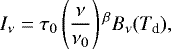
The first-order derivative function disappears in the case of any symmetrical temperature distributions like the Gaussian one. The three spectral components of Eq. (13) are displayed in the example of Fig. 1. While the component of index 1 can be of both signs, the component of index 2 is always positive for all frequencies and mostly influences the Wien part of the spectrum. The three components have the same Rayleigh-Jeans spectral behaviour in ∝ ν2 T0τν. The analogy to the Sunyaev-Zel’dovich (SZ) effect, a CMB spectral distortion in clusters of galaxies, is given in Appendix B. The complete formalism of the interaction of a temperature distribution with the Planck function was developed by Stebbins (2007). He shows that logarithm temperature moments are the key quantities to know, irrespective of the exact distribution, here p(t), as can be seen in our Eq. (12). Pitrou & Stebbins (2014) have argued for t ≡ ln T as the proper variable to use in the context of the CMB distortions (including relativity Lorentz frame invariance). We think that there is an additional reason for that use that is linked to the way photometric data are spread in frequency (see below).
2.3 Finding the underlying distribution of dust temperature from photometry
We now see the interest in the decomposition of the dust emission spectrum into the Planck function and its two derivatives (Eq. (13)). With only a few parameters, we can describe quite different situations. Photometricmeasurements are used to deduce dust properties, abundance, and luminosity. They are obtained from broadband detectors: photoconductors, bolometers, and kinetic inductance detectors (KIDs). The width of the band n, of a given instrument and telescope, described by the transmission curve Hn (ν), is so large that one has to assume a reference spectrum, Jν, to quote a brightness,  , at the band centralfrequency, νn, and for a given underlying spectrum, Iν:
 (15)
(15)
To simplify further, we define the set of normalised transmission functions for a given instrument as
![Mathematical equation: \[ G_{\nu}^{n}=\frac{J_{\nu_{n}}}{\int {\textrm{d}}\nu\thinspace H_{n}(\nu)\thinspace J_{\nu}}H_{n}(\nu)\thinspace, \]](/articles/aa/full_html/2022/03/aa42617-21/aa42617-21-eq20.png)
and we can rewrite the bandpass Eq. (15) as:
 (16)
(16)
where the bracket indicates a simple integration over the frequencies.
The reference spectrum, Jν, is usually taken as the first derivative of the CMB Planck function for millimetre wavelengths (including the 353 GHz Planck mission band),
![Mathematical equation: \[ J_{\nu}=\frac{P\nu^{3}}{T_{\textrm{CMB}}}g(\frac{h\nu}{kT_{\textrm{CMB}}}), \]](/articles/aa/full_html/2022/03/aa42617-21/aa42617-21-eq22.png)
and the Jν ∝ ν−1 Infrared Astronomical Satellite (IRAS) convention at submillimetre wavelengths. The ratio Iν (νn)∕In is close to one and is usually called the colour correction.
The bandpass Hn has a typical width of Δνn and is usually characterised by a resolution of  irrespective of νn. So the effective spectral resolution is coarse but constant in logarithm terms. It is thus appropriate to match this logarithmic scale with the temperature grid that we seek. For that purpose, it is worth remembering that dust cannot be colder than the CMB. Therefore, we propose discretising the temperature as follows:
 (17)
(17)
or Tl = TCMB.el.s, where l is an integer starting at 0 for the CMB temperature. The logarithmic temperature step, s, should match the photometric gridding, so values of  or
or  seem appropriate. The grid upper limit depends on the chosen experiments. Defining
  , and using Eq. (13), we can now rewrite the dust brightness as a linear decomposition of known functions that are fixed by the grid of Eq. (17):
![Mathematical equation: \begin{align*} I_{\nu} & =P\nu^{3}\sum_{l=0}\tau_{\nu}^{l}[f(x_{l})+\Delta t_{l}\,g(x_{l})\,\nonumber \\ & \quad +\frac{1}{2}\left(\Delta t_{l}^{2}+\sigma_{l}^{2}\right)\,g(x_{l})\,(h(x_{l})-1)],\end{align*}](/articles/aa/full_html/2022/03/aa42617-21/aa42617-21-eq28.png) (18)
(18)
where the l component is described byits opacity law,  , and its temperature distribution, which is solely characterised by two parameters: the logarithm mean temperature shift,
  , and the dispersion, σl. In order to compare the model with observations, we must take into account the passage of light through an instrument, by combining Eqs. (18) and (16). For that purpose, we normalise the opacity
  to a reference opacity, τl (say, at a given frequency). We can then define three series of coefficients, which describe the coupling between the dust temperature grid and the set of photometric bands:
![Mathematical equation: \begin{align*} K\prime_{0,n,l} & \equiv\left\langle G_{\nu}^{n}.\left[P\nu{{}^3}\frac{\tau_{\nu}^{l}}{\tau_{l}}f(x_{l})\right]\right\rangle, \end{align*}](/articles/aa/full_html/2022/03/aa42617-21/aa42617-21-eq32.png)
![Mathematical equation: \begin{align*} K_{1,n,l} & \equiv\left\langle G_{\nu}^{n}.\left[P\nu{{}^3}\frac{\tau_{\nu}^{l}}{\tau_{l}}g(x_{l})\right]\right\rangle, \end{align*}](/articles/aa/full_html/2022/03/aa42617-21/aa42617-21-eq33.png)
![Mathematical equation: \begin{align*} K_{2,n,l} & \equiv\left\langle G_{\nu}^{n}.\left[P\nu{{}^3}\frac{\tau_{\nu}^{l}}{\tau_{l}}g(x_{l})(h(x_{l})-1)\right]\right\rangle,\end{align*}](/articles/aa/full_html/2022/03/aa42617-21/aa42617-21-eq34.png) (19)
(19)
and we obtain the photometric expectation in band n:
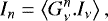
![Mathematical equation: \begin{align*} I_{n} & =\sum_{l=0}\tau_{l}[K\prime_{0,n,l}+\Delta t_{l}K_{1,n,l}+\frac{1}{2}\left(\Delta t_{l}^{2}+\sigma_{l}^{2}\right)K_{2,n,l}].\end{align*}](/articles/aa/full_html/2022/03/aa42617-21/aa42617-21-eq35.png) (20)
(20)
We now need a digression with respect to the first temperature bin at TCMB, which is going to modify K′.
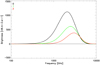 |
Fig. 1 Three elementary spectra of dust (see Eq. (13)) in a log-linear scale. For illustration purposes, we take the case of 20 K dust with an emissivity of
|
2.4 The radiative transfer of the CMB through dust
We now want to take into account the dominant background, which goes through interstellar dust before reaching the instruments1. It happens that dust, although a very thin layer with opacities much smaller than 1, has a non-negligible impact on the CMB and vice versa. The radiative transfer equation is solved for a single-temperature dust to get
![Mathematical equation: \[ I_{\nu}=B_{\nu}(T_{\textrm{CMB}})+(1-e^{-\tau_{\nu}})\left[B_{\nu}(T_{\textrm{d}})-B_{\nu}(T_{\textrm{CMB}})\right], \]](/articles/aa/full_html/2022/03/aa42617-21/aa42617-21-eq36.png)
which can be rewritten, for the optically thin case, as the real modified blackbody (RMBB) law:
![Mathematical equation: \begin{equation*} I_{\nu d}=\tau_{\nu}\left[B_{\nu}(T_{\textrm{d}})-B_{\nu}(T_{\textrm{CMB}})\right],\end{equation*}](/articles/aa/full_html/2022/03/aa42617-21/aa42617-21-eq37.png) (21)
(21)
where we have suppressed the CMB monopole term, which is cancelled out in the measurement by the current differential experiments, except the Far Infrared Absolute Spectrophotometer (FIRAS) on the Cosmic Background Explorer (COBE). The RMBB law is important in the millimetre domain. For example, at 100 GHz the correction amounts to a 7% downward effect for 18 K dust, irrespective of the emissivity law. The RMBB can be compared with the occultation of the CMB by planets, which is taken into account in the calibration of cold planets. Equation (21) is equivalent to saying that in Eq. (20) the first term,  , is special and has to be modified into
  so that very cold dust (at the CMB temperature) becomes invisible (a consequence of Kirchhoff’s law). The influence of the CMB on the submillimetre spectrum of high-redshift galaxies has also been noted by da Cunha et al. (2013). Here we show that, independent of redshift, the CMB has to be explicitly included in the dust SED.
We can now rewrite Eq. (20) as
![Mathematical equation: \begin{align*} I_{n} & =\sum_{l=0}\tau_{l}[K_{0,n,l}+\Delta t_{l}K_{1,n,l}+\frac{1}{2}\left(\Delta t_{l}^{2}+\sigma_{l}^{2}\right)K_{2,n,l}].\end{align*}](/articles/aa/full_html/2022/03/aa42617-21/aa42617-21-eq40.png) (22)
(22)
Although K0,n,0 = 0, very cold dust can still manifest itself with the other two CMB terms: K1,n,0 and K2,n,0. We note that it is more likely coming from the CIB than from interstellar dust. Elfgren & Désert (2004) have made a case for part of the CIB being in the spectral form encapsulated by the coefficients K1,n,0.
3 Discussion
We think that the result described in Eq. (22) is general enough to encompass the description of many dust environments. It includes the modified blackbody (MBB) case if there is only one l component, without dispersion (σl = 0). The data at hand in photometric bands  (with the associated error bar
  ) can be easily compared with this model. If we assume a dust emissivity law (identical or not for different l components), the coefficients K can be pre-computed once and for all, thus making the fitting process very fast for many lines of sight:
 (23)
(23)
If we keep only the first two coefficients, K0,n,l and K1,n,l, the fit is strictly linear, with the condition that c0,l must be positive. The number of components, as described by the number of useful l components, must be tuned in the process in order to keep  small. In that sense, the process is parsimonious: finding one l component that is best at minimising the χ2 and testing to see if a second one is really needed, then iterating. If we add the temperature distribution with K2,n,l and σl, and compare Eqs. (22) with (23), we can recover a linear fit if we include Lagrange coefficients to satisfy the condition
  .
.
The true non-linear part of the fit is in the emissivity law, which is hidden in the K coefficients. What is also hidden is the absolute calibration uncertainty of the instrument. This second set of values is degenerate with K. Another complication arises with the emissivity law, which is, in principle, different for different l. One can assume the same emissivity for a starter and refine that hypothesis if it happens to be really necessary. From Fig. 1 we see that a temperature spread always produces a positive distortion at all frequencies. The effect is that an MBB fit will tend to overestimate the dust temperature and to undervalue the emissivity index. So not only do we have statistically anti-correlated error bars between these two quantities (Shetty et al. 2009), but the (genuine) temperature spread along the line-of-sight can cause an apparent T-β anti-correlation too.
One could find that this model has ‘too many’ parameters. But we would argue that for the case  , this corresponds to only five discrete temperatures between 8 and 30 K, namely 9.1, 12.2, 16.5, 22.3, and 30 K. Secondly, the fitting procedure can cull the components as the parameters in Eq. (23) have to conform to positivity constraints set by Eq. (22). With the case shown in Fig. 1, a single-temperature logarithmic change by
  yields a maximum residual of 0.6% relative to the peak emission for three components fitted with Eq. (23) (3.5% if only two components are used).
Another constraint will show up when one finds that the temperature spread is larger than the bin size, s. In that case, the parameter σ should saturate to  (the equivalent of uniform noise in a digital binning process), and hence
  .
.
The bolometric luminosity of dust can be directly computed from a linear combination of integrals pre-computed from Eq. (18). Polarisation photometry follows the same rules as intensity. We can expect the degree of dust polarisation to be strong when the temperature distribution is not too spread out (i.e. for small σ).
The CIB fluctuations (Planck Collaboration XXX 2014) may be revisited in light of this model because of the linearisation procedure, as it can lend itself to the powerful statistical tools used for CMB studies, including covariances and model testing with likelihood functions, via the statistics of the ci,l coefficients.
This work is complementary to the approach by Chluba et al. (2017). Both studies put the emphasis on Planck derivatives and temperature moments. Chluba et al. (2017) argues for  as the proper expansion variable. Weprefer ln T because it will fare better, in terms of the number of required steps in the temperature grid, for broad temperaturedistributions (including the CIB and the example in Sect. 1), where more than one l component is necessary. In that case, high-frequency convergence problems, signalled by Chluba et al. (2017), are also alleviated. Moreover, for broadband experiments, it is impossible to go beyond the second Planck derivative as the fitting system becomes too under-determined for limited signal-to-noise ratio measurements.
4 Conclusions
We have shown an analytical development around the Planck function. We have emphasised the role of its second derivative with respect to the logarithm of the dust temperature. This is important in order to include the effect of a very likely distribution of temperatures along the line-of-sight around the main dust temperature. We have also devised an economical way of accounting for a wider temperature range by discretising the temperature ladder in constant logarithm steps, which naturally starts at the CMB temperature. By explicitly including the instrumental measurement process, we have devised a model that can be fit in an almost linear way, from photometry to dust temperature distributions, thus accelerating the computation of the inverse problem. Further work will have to be done to implement these findings for the analysis of dust in the Planck and Herschel missions, in particular the optimal gridding of dust temperatures versus the experimental photometric frequency sampling. This work is complementary to investigations of the possible variations in the emissivity index in some galactic regions (Mangilli et al. 2021; Rigby et al. 2018; Bracco et al. 2017; Tang et al. 2021; Planck Collaboration Int. XIV 2014). Applications to the CIB statistics and dust as the major foreground for CMB studies should be sought too.
Acknowledgements
The author thanks discussions with François-Xavier Hamel, Guilaine Lagache and Nicolas Ponthieu.
Appendix A Planck derivative functions
The third Planck derivative is useful for assessing the errors made by using only two derivatives in the Taylor expansion. For completeness, it is given here:
![Mathematical equation: \begin{equation*} \frac{d^{3}B_{\nu}}{dt^{3}}=P\nu^{3}g(x)\left[(h(x)-1){}^{2}-h(x)+2x\,g(x)\right].\end{equation*}](/articles/aa/full_html/2022/03/aa42617-21/aa42617-21-eq51.png) (A.1)
(A.1)
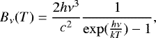
It is worth showing the graph of Planck derivative functions. As they all diverge at low frequencies as  , we can show instead x times the functions. In Fig. A.1 we show the Planck function and its three derivatives (with the index going from 0 to 3).
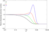 |
Fig. A.1 Four Planck functions (times x) as a functionof the dimensionless frequency parameter x. The Planck function has the 0 index, and the three indices label the three consecutive Planck function derivatives. Hence, we have plotted x f(x), x g(x), x g(x) (h(x) − 1), and |
![Mathematical equation: $x\,g(x)\,\left[(h(x)-1){}^{2}-h(x)+2x\,g(x)\right]$](/articles/aa/full_html/2022/03/aa42617-21/aa42617-21-eq58.png)
Appendix B The Sunyaev-Zel’dovich effect
The second derivative of the Planck function is linked to the SZ effect, a spectral distortion of the CMB through clusters of galaxies. The SZ effect is quantified by the Compton parameter, y, which is proportionalto the integrated thermal electron pressure along the line-of-sight. Indeed, if we specifically perform the substitution Δt = −3y and σ2 = 2y in Eq. 13, where T0 = TCMB is the present CMB temperature (Stebbins 2007), we recover the SZ non-relativistic thermal distortion:
 (B.1)
(B.1)
This gives a direct interpretation of the SZ distortion: the Compton effect (while maintaining the number of photons constant) shifts the CMB average temperature along the cluster line-of-sight by a relative factor of − 3y, and the Maxwellian electron velocity distribution interacts with the CMB photons as if they produced a Gaussian temperature distribution with a dispersion σ. This explains why the quadratic equivalent temperature dispersion in logarithm is proportional to the quadratic Maxwellian velocity distribution (i.e. the electron temperature, Te): 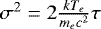 , where me is the electron mass and τ is the line-of-sight opacity to the Compton effect.
One of the differences between the SZ spectral distortion (in h − 4) and the Planck second derivative (in h − 1) is that the SZ effect has a negative relative distortion in the Rayleigh-Jeans part of the spectrum, the so-called SZ decrement:  .
.
References
- Bracco, A., Palmeirim, P., André, P., et al. 2017, A&A, 604, A52 [NASA ADS] [CrossRef] [EDP Sciences] [Google Scholar]
- Chluba, J., Hill, J. C., & Abitbol, M. H. 2017, MNRAS, 472, 1195 [NASA ADS] [CrossRef] [Google Scholar]
- da Cunha, E., Groves, B., Walter, F., et al. 2013, ApJ, 766, 13 [Google Scholar]
- Elfgren, E., & Désert, F. X. 2004, A&A, 425, 9 [NASA ADS] [CrossRef] [EDP Sciences] [Google Scholar]
- Galliano, F., Galametz, M., & Jones, A. P. 2018, ARA&A, 56, 673 [Google Scholar]
- Hensley, B. S., & Draine, B. T. 2021, ApJ, 906, 73 [NASA ADS] [CrossRef] [Google Scholar]
- Mangilli, A., Aumont, J., Rotti, A., et al. 2021, A&A, 647, A52 [NASA ADS] [CrossRef] [EDP Sciences] [Google Scholar]
- Pitrou, C., & Stebbins, A. 2014, Gen. Relativ. Gravit., 46, 1806 [CrossRef] [Google Scholar]
- Planck Collaboration XXX. 2014, A&A, 571, A30 [NASA ADS] [CrossRef] [EDP Sciences] [Google Scholar]
- Planck Collaboration Int. XIV. 2014, A&A, 564, A45 [NASA ADS] [CrossRef] [EDP Sciences] [Google Scholar]
- Rigby, A. J., Peretto, N., Adam, R., et al. 2018, A&A, 615, A18 [NASA ADS] [CrossRef] [EDP Sciences] [Google Scholar]
- Shetty, R., Kauffmann, J., Schnee, S., Goodman, A. A., & Ercolano, B. 2009, ApJ, 696, 2234 [Google Scholar]
- Stebbins, A. 2007, ArXiv e-prints, [arXiv:astro-ph/0703541] [Google Scholar]
- Tang, Y., Wang, Q. D., & Wilson, G. W. 2021, MNRAS, 505, 2377 [NASA ADS] [CrossRef] [Google Scholar]
This study was reported to the Planck mission consortium in 2014 but was never published.
All Figures
|
Fig. 1 Three elementary spectra of dust (see Eq. (13)) in a log-linear scale. For illustration purposes, we take the case of 20 K dust with an emissivity of
|
| In the text | |
|
Fig. A.1 Four Planck functions (times x) as a functionof the dimensionless frequency parameter x. The Planck function has the 0 index, and the three indices label the three consecutive Planck function derivatives. Hence, we have plotted x f(x), x g(x), x g(x) (h(x) − 1), and |
| In the text | |
Current usage metrics show cumulative count of Article Views (full-text article views including HTML views, PDF and ePub downloads, according to the available data) and Abstracts Views on Vision4Press platform.
Data correspond to usage on the plateform after 2015. The current usage metrics is available 48-96 hours after online publication and is updated daily on week days.
Initial download of the metrics may take a while.