| Issue |
A&A
Volume 659, March 2022
|
|
|---|---|---|
| Article Number | A82 | |
| Number of page(s) | 11 | |
| Section | Interstellar and circumstellar matter | |
| DOI | https://doi.org/10.1051/0004-6361/202142334 | |
| Published online | 09 March 2022 | |
Dust scattering halo around the CCO in HESS J1731–347: A detailed analysis
Institute for Astronomy and Astrophysics, Kepler Center for Astro- and Particle Physics, Eberhard Karls University,
Sand 1,
72076
Tübingen,
Germany
e-mail: This email address is being protected from spambots. You need JavaScript enabled to view it.
Received:
29
September
2021
Accepted:
27
January
2022
Abstract
The supernova remnant (SNR) HESS J1731−347 is one of the few objects exhibiting emission up to the TeV energy band and it stands as a prime target for the study of cosmic ray acceleration in SNRs. It also hosts a central compact object (CCO), which is of interest in the context of the ultra-dense matter equation of state in neutron stars. For both types of studies, however, the parameters of the respective models depend crucially on the assumed distance to the object and are affected to a certain extent by the assumed interstellar medium (ISM) properties around the SNR. Here, we report on the first quantitative analysis of the properties of the compact X-ray dust scattering halo that is assumed to be present around the CCO based on Chandra observations of the source. Our findings unambiguously confirm the presence of a compact halo around the CCO, and we show that the observed halo properties are consistent with expectations from independent measurements of the dust distribution along the line of sight and the distance to the source. Although we were not able to significantly improve those constraints, our results are important for future studies of the CCO itself. Indeed, the halo contribution is expected to affect the X-ray spectrum and the derived parameters of the neutron star when observed with moderate angular resolutions. Our results, which offer a quantitative characterization of the halo properties, will be useful in accounting for this effect.
Key words: stars: neutron / X-rays: general / ISM: supernova remnants / scattering
© ESO 2022
1 Introduction
The supernova remnant (SNR) HESS J1731−347 was discovered with the High Energy Stereoscopic System (H.E.S.S.) and is one of the few SNRs which, besides exhibiting radio synchrotron, also exhibits non-thermal X-ray and TeV emission (H.E.S.S. Collaboration 2011). This points to effective and ongoing particle acceleration and, thus, to a young age of the remnant (≈104 yr). Two scenarios have been considered to explain the observed very high-energy (VHE, ≳100 GeV) emission from the shell, namely: inverse Compton emission from relativistic electrons accelerated in the SNR shocks (“leptonic” scenario) or π0-decay from shock-accelerated protons (“hadronic” scenario). The latter is particularly appealing as it may help to pinpoint young SNRs as the main source of cosmic ray acceleration (H.E.S.S. Collaboration 2011). HESS J1731−347 is just one of a handful of objects where substantial evidence for the hadronic mechanism of TeV production has been offered.
Besides the cosmic ray acceleration, this SNR is also extremely interesting in the context of isolated neutron star studies (Klochkov et al. 2013, De Luca 2017). The remnant hosts a centrally located, radio-quiet, thermally X-ray emitting isolated neutron star with no detectable pulsations in the X-ray band. Such neutron stars are usually referred to as central compact objects (CCOs) and they are prime targets in studies of the equation of state of ultra-dense matter found in neutron stars (Klochkov et al. 2013, 2015). To fully exploit both science cases, a robust estimate of the distance to the object is essential.
As discussed by H.E.S.S. Collaboration (2011), the SNR is likely located in one of the Galactic spiral arms along the line of sight, which implies a location at either ~3 kpc (Norma arm), ~4.5 kpc (Scutum-Crux arm), or 5–6 kpc (3 kpc arm) distance from Earth. Larger distances beyond the Galactic center are disfavoured by arguments of the SNR’s energetics. From a comparison of the X-ray absorption column to several regions of the SNR with the expected absorption from atomic and molecular hydrogen integrated to different distances, H.E.S.S. Collaboration (2011) derived a lower distance limit of 3.2 kpc, placing HESS J1731−347 at the rear side of the Norma arm or beyond. This conclusion was corroborated by the observed alignment of dense clumps seen in carbon monosulfide (CS) and in infrared (IR) absorption with the SNR (Maxted et al. 2015, 2018; Doroshenko et al. 2017) and through a refined X-ray absorption analysis that also allowed Maxted et al. (2018) to exclude much larger distances. On the other hand, an upper limit of 4.5 kpc was estimated by Klochkov et al. (2013, 2015) based on the modeling of the compact object’s X-ray spectrum. We note that all of these estimates are in conflict with an association of the SNR with the 3 kpc arm and the implied distance of 5–6 kpc, as proposed by Fukuda et al. (2014). On the other hand, besides the 4.5 kpc upper limit, all estimates mentioned above depend on the assumed rotation curve of the Galaxy as the distance to the absorbing material was estimated based on the observed velocities of gas deduced from radio observations.
From a completely different perspective, the identification of a star in the optical band which is unambiguously associated with the SNR (Doroshenko et al. 2016) provided independent and more accurate ways to estimate the distance to all three objects. On the one hand, using the observed spectral energy distribution (SED) of the star itself and the massive dust shell surrounding it and illuminated by it, Doroshenko et al. (2016) estimated a distance of 3.8(7) kpc. On the other hand, in theGaia EDR3 release (Gaia Collaboration 2020; Bailer-Jones et al. 2021), a geometric distance of 2.5(3) kpc and a photo-geometric distance of 2.4(2), slightly lower than the other estimates discussed above, are reported.
H.E.S.S. Collaboration (2011) argued that the absorption pattern towards HESS J1731−347 is dominated by a molecular cloud (seen in carbon monoxide, CO) at 3.2 kpc distance in the line of sight towards the western part of the SNR, but from the lack of correlation of the TeV emission with the gas, they concluded that the remnant should not be in contact with the gas but is located behind it. On the other hand, as cited above, there is good evidence of an alignment of some gas tracers with the SNR in the same region of the SNR, and Doroshenko et al. (2017) even argued that there is evidence that the SNR is partially embedded in the 3.2 kpc cloud. This would support the case for a hadronic origin of at least a fraction of the observed TeV γ-ray emission. On the other hand, a repeated spatial correlation analysis between the observed X-ray absorption and the integrated CO emission in the same direction, carried out by Doroshenko et al. (2017), found that while the correlation significance vanishes beyond local standard of rest velocities υLSR ~−25 km s−1 (in agreement with the 3.2 kpc lower limit), the correlation remains high over the full range of lower velocities. This would suggest that the absorbing material is not necessarily concentrated at ~3 kpc, but may be more homogeneously distributed between this distance and the observer. Similarly, while the near-IR extinction in the direction of the SNR (Fig. 8 of Doroshenko et al. 2017) shows a peak near 3 kpc, the distribution might also indicate that the material is more widely distributed between source and observer.
Dust scattering halos around bright sources provide an alternative means of probing the material distribution between the source and the observer (Predehl et al. 1995), assuming that the gas-to-dust ratio stays constant along the line of sight or can be estimated, to the level of necessary accuracy. The presence of a dust scattering halo around the CCO in HESS J1731-347 has already been casually suggested by Halpern et al. (2010), but neither the halo interpretation nor a detailed analysis of its properties have been quantitatively justified up to now. Here, we report the first quantitative analysis of this kind, using Chandra data. To assess the accuracy by which the location of the target material can be probed through its co-located dust properties is one of the prime goals of the presented work.
In Sect. 2, we describe the observations and the data analysis and report the basic observed properties of the halo. In Sect. 3, we investigate the halo properties in detail and model its observed radial profile to investigate the distribution of the material along the line of sight and to either obtain an estimate of the relative distance of the scattering region or an estimate for the absolute distance to the CCO itself. In Sect. 4, we discuss the implication of the results.
2 Data analysis
The spatial analysis of the dust scattering halo presented below is based on Chandra observations of the source performed on April 28, 2008 and on April 4, 2021. These two observations are the longest Chandra observations of the source available, and furthermore, the prime goal of the second observation was to estimate the expansion rate of the SNR through differential imaging, and thus it was specifically set up to replicate the first observation with the highest accuracy possible to avoid potential systematic effects associated with a variation in the instrument’s point spread function (PSF) across the field of view.
As a first step, we conducted a standard spatial analysis and reduced the data using the Chandra Interactive Analysis of Observations software (CIAO v4.9, Fruscione et al. 2006). The raw data were reprocessed using the chandra_repro script, and the deflare script was used to remove background flaring in the observation. The effective exposure with the Advanced CCD Imaging Spectrometer (ACIS-I) after filtering amounted to 29.23 ks1, and 33.62 ks2, for the two observations, respectively. To detect the CCO and possible other sources (to remove them) and to estimate their positions, we used fluximage and wavdetect tools, respectively. Using the coordinates of the detected sources, both observations were then accurately aligned and merged using the merge_obs task. This allowed us to increase counting statistics when constructing the radial profile of the halo. The obtained sky map around the CCO is shown in Fig. 1.
Before proceeding to the analysis of the halo properties, we verified that the interpretation of the faint extended emission around the CCO as a dust scattering halo by Halpern et al. (2010) is indeed valid. In addition, we verified thatpotential alternative interpretations, such as a possible pulsar wind nebula (PWN) around the neutron star or locally enhanced extended emission from the SNR, are not consistent with the data. The spectrum of the observed emission appears to be rather soft and definitively inconsistent with a potential origin as part of the extended SNR emission or a PWN candidate. To illustrate that, we extracted source and background spectra from θ = 10″−30″ and θ = 50″−70″ annuli centered on the CCO (separately for both observations, co-adding results using the combine_spectra task), whichis shown in Fig. 2. The observed spectrum is consistent with a blackbody with kT = 0.41(3) keV (with NH = 1.7(3) × 1022 atoms cm−2 and χ2/d.o.f. = 31.12/34), that is, slightly softer than that of the CCO (0.5 keV, Klochkov et al. 2013), which is as expected for scattered emission. We emphasize that while the observed spectrum can also be formally modeled with a power law (with photon index Γ = 5.5(5), NH = 3.5(5) × 1022 atoms cm−2 and χ2/d.o.f. = 26.53/34), the resulting values for the photon index and absorption column are way too large to be related to the extended SNR emission or a potential PWN. Indeed, Doroshenko et al. (2017) reported a photon index of 2.66 withno significant variations over the SNR shell. Compact PWNe have an even harder spectrum (Γ ~ 1−2; Kargaltsev et al. 2015). Therefore, a scattering halo appears to be the only feasible interpretation.
In the next step, the radial profile of the emission around the CCO was extracted (this includes both the contribution of the point sourceand the dust scattering halo). Photon counts in 32 linearly spaced concentric annuli around the CCO for θ = 0−120″ were co-added and divided by the area of the respective region to obtain the surface brightness profile shown in Fig. 3. The contribution of the suggested companion of the CCO (Doroshenko et al. 2016) and another nearby point source was removed by masking the pixels within 5′′ from their location, respectively, as shown in Fig. 1. Considering the faintness of the halo with respect to the central point source, even a minor contribution of the latter in the wings of the instrument’s PSF is not negligible and needs to be accurately estimated and accounted for when modeling the observed radial profile. In practice, this means that the location in the detector plane, the source spectrum and the energy dependence of the instrument’s PSF need to be considered to estimate the point source contribution in a given energy range.
To do so, we first extracted the energy spectrum of the CCO using the specextract script and used this along with the measured position of the source as an input for the Chandra ray-tracer ChaRT v2 (Carter et al. 2003). Other parameters of the simulation were set to replicate the actual observations (which have an identical configuration) as described in the ChaRT2 documentation3. The aim of the simulation is to accurately estimate the expected contribution of a single point source with the spectrum and the position identical to that of the CCO to the observed image considering the energy dependence of the PSF. To do that, we used used the MARX package (Davis et al. 2012) to construct, based on the simulated photon list, an image containing only the point source, and then extracted its radial profile in the same way as described above for the observed radial profile. To improve counting statistics for the simulated PSF images, we increased the simulated exposure by a factor of 50 (with respect to the combined exposure of both observations used in the analysis), as recommended in the ChaRT2 documentation, and then divided the obtained radial profile of the point source by the same factor. The simulated PSF is also shown in Fig. 1.
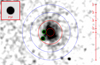 |
Fig. 1 Adaptively smoothed count image (derived from Chandra data) around the CCO showing the brightest part of the halo, with the simulated PSF (scaled accordingly) on top left. Additionally, the image is smoothed with a 5′′ kernel (which corresponds to the size of the small green circles denoting two point sources excluded from the analysis) to enhance the visual appearance. The red and blue annuli denote the source and background regions that were used to extract the halo spectrum, respectively. Within the source region, the contribution of the CCO is negligible, as also illustrated in Fig. 3. |
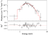 |
Fig. 2 Unfolded spectrum (black) and best-fit black body model (red) of the extendedhalo emission extracted from an annulus with inner and outer radii of 10′′ and 30′′, as describedin the text and residuals to the best fit (lower panel). |
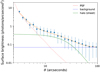 |
Fig. 3 Final newdust model (thin sheet approximation) of the halo (green), data points obtained from the observation (blue, with error bars), and the simulated image (red). All added components (orange) match the observation best with the derived parameters. |
3 Modeling
The extension of an X-ray halo depends mostly on the dust parameters and the distribution of dust between the source and the observer (Smith et al. 1998) and, thus, can be used to probe those. Several useful analytic approximations exist to describe the expected halo radial profile for simple cases, namely, for uniformly distributed dust or scattering in a thin sheet of dust somewhere between the source and the observer (Draine 2003). In the latter case, the halo extension is largest when the dust cloud is located close to the observer and gets more compact when the scatterer gets closer to the source (Draine 2003; Fig. 4). Moving then from relative to absolute distances, the modeling of the halo’s radial profile could thus be used to either constrain the distance to the source (if the distance to the scatterer were known) or to locate the scattering material (if the distance to the source were known).
In the case of the SNR HESS J1731−347, the halo around the CCO with an extension of only several tens of arc seconds (see below) appears to be rather compact (X-ray scattering halos are typically much larger and can extend up to thousands of arcseconds; Lamer et al. 2021). This means that the estimated dust distribution is a representative of the absorbing material towards the center of the SNR, and suggests a dominant contribution from a rather compact dust sheet close to the source. We model four potential distributions: a thin dust sheet somewhere between the source and the observer (i.e., only a contribution of a compact cloud such as the one seen towards the West of the SNR); a uniform distribution; a combination of the former two cases (reflecting some of the results in Doroshenko et al. 2017); and a realistic dust distribution which is derived from 3D extinction maps published by Lallement et al. (2019). In all cases, the dust density perpendicular to the line of sight was assumed to remain constant on scales that are relevant to the formation of a scattering halo.
In all four cases, the observed radial profile was modeled as a combination of a contribution from the point source, the background emission from the SNR, and the halo radial profile calculated for each case as described below. In all cases, in addition to the parameters describing the halo properties, we assumed the scaling of the simulated PSF and the background level to be free parameters to account for possible minor discrepancies between the absolute flux derived from the simulation and the actual observation and for possible spatial variations in the SNR emission (which would not be possible if the background would be simply subtracted using an off-source region). The modeling was conducted using the Bayesian inference nested sample package ultranest4 (Buchner 2021), which allows for the evaluation of marginal likelihoods (i.e., global Bayesian evidences) and thus meaningful comparisonsof non-nested models. For all described cases of dust distribution, details on the modeling and the results are given in the following.
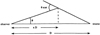 |
Fig. 4 Schematic drawing of the X-ray scattering geometry, whereby D denotes the distance to the source, xD the distance to the scattering cloud, θ the opening angle of the halo, and θscat the scattering angle (Mathis & Lee 1991). |
3.1 Thin sheet approximation
We considered two options to model the scattering halo’s radial profile using a thin sheet approximation in order to check the consistency of the modeling. First, we used the simple analytical approximation by Draine (2003), where the scattering cross section is approximated by use of a “median” scattering angle θs,50 for a given dust composition, which is expected to be a reasonably good approximation for photon energies E > 1 keV (and thus is satisfied in our case as most of the photons below this energy are in any case absorbed). For the WD01 dust composition (Weingartner & Draine 2001), we have θs,50~ 360′′ keV/E, and the differential scattering cross section is given by
![Mathematical equation: \begin{equation*} \frac{\textrm{d}\sigma}{\textrm{d}\Omega}\approx\frac{\sigma_{\textrm{sca}}}{\pi\theta^2_{\textrm{s,50}}\left[1+\left(\theta/\theta_{\textrm{s,50}}\right)^2\right]^2}. \end{equation*}](/articles/aa/full_html/2022/03/aa42334-21/aa42334-21-eq1.png)
If the scattering of X-rays from a point source at a distance D occurs in a thin sheet at a distance r = xD * D, a halo around the point source with the halo angle θh ~ (1 − xD)θs is produced, and the fraction of halo photons within this angle (i.e., the cumulative radial profile) g(θh) = Nhalo(≤ θh)∕Nhalo can be estimated as
In practice, we calculated the value of this function for each of the annuli used to obtain the observed differential radial profile, and subtracted the contribution of the inner parts from that of the outer parts to match the model with the data. The total halo intensity is then defined by the scattering optical depth τsca = ln(1 + Nhalo)∕Nsrc, which makes the model only dependent on the absorption column, the photon energy, E, the photon counts of the point source and the relative distance to the scatterer, xD. The scattering optical depth can also roughly be expressed as  (Corrales et al. 2016). This allowed us to use the absorption column derived from the spectral analysis of the CCO at NH = 2.00(3) × 1022 cm−2 (Klochkov et al. 2015) to define a Gaussian prior for the scattering optical depth (using a mean of 2 and a standard deviation of 0.03 for NH), which remained, however, a free parameter (denoted as NH below). For the other free parameters, namely, the background level (Abkg), the PSF scaling (APSF), and the relative distance to the scatterer xD, the following priors were assumed: a Gaussian prior with a mean of 1 and a standard deviation of 0.1 for PSF scaling, a Gaussian prior with a mean equal to the flux in the outermost ring and a standard deviation of half of that for the background, and a uniform prior in the range of [0...1] for xD.
We note that the assumption of constant energy we made above is, strictly speaking, not correct, and, in principle, we need to integrate over the spectrum of the scattered emission. Indeed, the halo profile itself, the PSF, and the effective area of a real telescope are all energy dependent, so neglecting this might lead to a distortion of the halo profile and thus lead to biased estimates. In our case this is not expected to be of significant importance as most of the source photons are detected in a relatively narrow energy band between 1 and 2 keV, but we still considered a more sophisticated numerical model for dust scattering (where integration over the energies is already implemented) developed by Corrales (2015) and available as the newdust code5 to verify if thisis indeed the case. We also took this opportunity to explore how using a different dust composition would affect the results (for the analytic model discussed above the WD01 dust composition is implicitly assumed). In particular, MRN (Mathis et al. 1977)was used for the modeling with the newdust code. The total scattering column in newdust is defined in units of g cm−2, so we adopted the same conversion of NH to mass as Corrales (2015), that is, we assumed
For both models, we limited the energy range to 1.2−2.5 keV for the analysis (i.e., we extracted radial profiles in this energy range), as this is reasonably close to be monochromatic, while still accounting for ~ 60 % of the CCO’s emitted photons. The best fit parameters for both models are reported in Table 1, and the posterior corner plots in Appendix A (which suggest to increase xD a bit, as it is clustered towards xD ≈ 0.8). The best-fit model profile for the newdust model is also shown in Fig. 3. As evident from Table 1, both models produce similar results and fit quality (as follows from the comparable marginal likelihoods log Z for each model) and adequately describe the observed radial profile. The observed halo intensity is consistent with the expected level given the observed X-ray absorption column, and the dust is concentrated towards the compact object as expected. Considering the greater detail of modeling with newdust, however, only the results obtained with this model are used below and for the modeling of other possible dust distributions.
Parameters of the best-fit Draine and newdust models considering different scattering components.
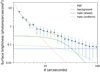 |
Fig. 5 Final newdust model (thin sheet + uniform distribution) of the halo (green), data points obtained from the observation (blue, with error bars), and the simulated image (red). All added components (orange) match the observation best with the derived parameters. |
3.2 Uniformly distributed dust approximation
So far, we have shown that if the majority of the scattering dust is (roughly) concentrated in one thin sheet, this sheet must be located close to the source, in line with a cloud in the Norma arm as suggested in H.E.S.S. Collaboration (2011) towards the West of the SNR. In a next step, we used the uniformly distributed dust model which is also implemented within the newdust code. In addition, wealso considered a combination of the two scenarios, namely: uniformly distributed dust plus a thin sheet at xD (Fig. 5). The modeling was conducted in the same way and with the same priors as described above for the thin sheet approximation, with the exception that xD is obviously not appearing in the purely uniformly distributed dust model. On the other hand, for the combined model, there is another parameter, namely, the fraction of uniformly distributed dust, funi/total, that appears. For this parameter, a uniform prior in range of [0...1] was used, whereas the prior derived from the observed X-ray absorption was still used for the total dust column as described above for the thin sheet approximation.
In both cases, it was possible to obtain an adequate fit with a level of quality similar to that for the thin sheet approximation (see Table 1 and Appendix A). This suggests that the quality of the available data does not allow us to discriminate between uniformly distributed dust and dust concentrated in a thin sheet. This conclusion is supported by the derived posterior distribution for funi/total in the combined model, which appears to spread over the entire allowed range. We note, however, that the posterior corner plot of the combined model (Fig. A.4) shows a wide spread of allowed values for xD, with the most probable values exhibiting xD ≥ 0.8.
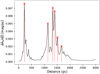 |
Fig. 6 Extinction along the line of sight in the direction to the CCO as reported in Lallement et al. (2019). The red vertical lines and crosses denote the locations and the relative amplitudes of the six thin sheets used to approximate the dust distribution for modeling of the halo radial profile. |
3.3 Realistic dust distribution
Considering that we were not able to arrive at a definitive conclusion regarding the dust distribution along the line of sight based on the analysis of the halo radial profile alone, we also attempted to incorporate prior information from other sources to obtain an improved distance estimate to the source. In particular, we used the 3D optical extinction maps based on Gaia and 2MASS data that were recently published by Lallement et al. (2019). We extracted the differential extinction profile along the line of sight in the direction to the CCO from the data cubes published by Lallement et al. (2019) and approximated it with six thin sheets corresponding to the most significant peaks in the obtained profile as illustrated in Fig. 6. We then assumed fixed distances to the individual sheets and the amount of material in each sheet was assumed to be proportional to the respective peak’s amplitude. The halo profile was then modeled as a sum of halos produced by each of the sheets using the Corrales (2015) model. The free parameters of the model were then set as the total amount of absorbing material, NH, (distributed among all six sheets) and the distance to the source D (which defines the relative distance for each of the sheets). Finally, similarly to the sheet and uniform models above, we also utilized the available prior information on the total scattering column. The results of the fit are presented in Fig. A.5 and Table 1.
As can be seen, the posterior distance estimate is fully consistent with the Gaia parallax estimate, so we conclude that the observed halo profile is consistent with what is expected from the estimated dust distribution along the line of sight and the observed absorption column. Additionally, the fitting quality analysis (Table 1) implies that this distribution is slightly more favorable than the previously mentioned ones given that it has the same number of free parameters.
4 Discussion and conclusions
Using archival Chandra observations, we were able to unambiguously confirm the presence of a scattering halo around the CCO and, for the first time, to quantitatively model it. In particular, we considered several alternative possibilities for the location of the scattering material, namely, assuming that: most of the scattering material is either confined to a thin sheet of dust somewhere between the X-ray source and the observer; distributed uniformly; a combination of the previous two possibilities; or a more realistic dust distribution derived from 3D optical extinction maps published by Lallement et al. (2019). Given previous reports, the fact that the X-ray absorption column towards the CCO is close to the maximum absorption towards the west of the SNR, and also taking into account the high angular-resolution gas maps of Maxted et al. (2018), we anticipated that the first possibility might be realized also in the line of sight towards the CCO, which would allow us to obtain an independent distance estimate to the CCO as the distance to the molecular cloud, which is likely to contain most of the scattering material is more or less known from radio measurements.
To model the halo radial profile, we used models developed by Draine (2003) and Corrales (2015). For the thin sheet approximation, both models yielded an estimated relative distance to the scatterer of xD ≈ 0.8 (Appendix A), namely, suggesting that it must be located close to the source. On the other hand, we also investigated the possibility of a uniform dust distribution, and a combination of both, uniformly distributed dust plus some material in a thin sheet, and found that both of these provide a similarly good description of the observed halo profile from a statistical point of view. Moreover, the combined model consisting of a thin sheet of dust plus some uniform composition was found to be weakly dependent on the assumed dust fraction in the sheet, which also strongly suggests that the available counting statistics is insufficient to discriminate between uniformly distributed dust and dust concentrated in a thin sheet.
Therefore, the only possibility to constrain the source distance is to adopt a dust distribution estimated from independent data. To this end, we used the 3D optical extinction maps from Lallement et al. (2019) and obtained a distance estimate to the CCO of DCCO = 2.79(62) kpc, which is fully independent of any of the estimates described in the introduction. The result is consistent with the Gaia parallax estimate to the counterpart. The latter model is also a slightly better description of the halo even if other representations are also fully consistent with the data. Most importantly, the presence of a compact scattering halo around the CCO was, for the first time, convincingly demonstrated and its parameters were quantitatively characterized.
We emphasize that the mere presence of the compact halo is an interesting result in itself, as most of its flux falls within the PSF of XMM-Newton telescopes, which, in the past, were used to constrain neutron star parameters through spectral analyses. Although the contribution of the halo to the observed spectrum is not large, it is expected to be significantly softer than the spectrum of the CCO itself and, thus, it could affect the observed spectral shape and potentially the conclusions drawn by Klochkov et al. (2013) and Suleimanov et al. (2014). We argue, therefore, that the presence of the halo must be accounted for in future investigations of the X-ray spectrum of the CCO in HESS J1731-347 and, possibly, other similar objects with significant absorption along the line of sight as well, using instruments with a moderate angular resolution such as XMM-Newton. The halo parameters reported here are based on the analysis of high-resolution Chandra imaging, proving to be useful for this purpose since a reconstruction of these based on the spectroscopy data alone might be problematic.
Acknowledgements
A.L. is supported by the German Aerospace Center (DLR, grant 50OR 1704). This work has made use of data from the European Space Agency (ESA) mission Gaia (https://www.cosmos.esa.int/gaia), processed by the Gaia Data Processing and Analysis Consortium (DPAC, https://www.cosmos.esa.int/web/gaia/dpac/consortium). Funding for the DPAC has been provided by national institutions, in particular the institutions participating in the Gaia Multilateral Agreement. This research has made use of data obtained from the Chandra Data Archive and the Chandra Source Catalog, and software provided by the Chandra X-ray Center (CXC) in the application packages CIAO and Sherpa.
Appendix A Figures
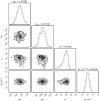 |
Fig. A.1 Posterior corner plots of the Draine model. Although clustered towards xD ≈ 0.8, lower values are allowed. |
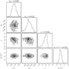 |
Fig. A.2 Posterior corner plots of the newdust thin sheet model. Although clustered towards xD ≈ 0.8, lower values are allowed. |
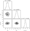 |
Fig. A.3 Posterior corner plots of the newdust pure uniform model. |
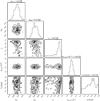 |
Fig. A.4 Posterior corner plots of the newdust combined uniform + thin sheet model. The wide spread of the dust mass fraction f (uni/total) implies that there is no clear preference towards any of both, i.e., modeling is possible with each of the components only. |
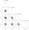 |
Fig. A.5 Posterior corner plots of the newdust model assuming a realistic dust distribution along the line of sight taken from Lallement et al. (2019) and priors on the total absorption column from Klochkov et al. (2015). |
References
- Anders, F., Khalatyan, A., Chiappini, C., et al. 2019, A&A, 628, A94 [NASA ADS] [CrossRef] [EDP Sciences] [Google Scholar]
- Arnaud, K. A. 1996, ASP Conf. Ser., 101, p17 [NASA ADS] [Google Scholar]
- Bailer-Jones, C. A. L., Rybizki, J., Fouesneau, M., et al. 2021, AJ, 161, 147B [NASA ADS] [CrossRef] [Google Scholar]
- Buchner, J. 2021, JOSS, 6, 3001 [NASA ADS] [CrossRef] [Google Scholar]
- Buchner, J., Georgakakis, A., Nandra, K., et al. 2014, A&A, 564, A125 [NASA ADS] [CrossRef] [EDP Sciences] [Google Scholar]
- Carter, C., Karovska, M., Jerius, D., et al. 2003, ASP Conf. Ser., 295, 477 [NASA ADS] [Google Scholar]
- Corrales, L. 2015, Astrophysics Source Code Library [record ascl:1503.005] [Google Scholar]
- Corrales, L. R., García, J., Wilms, J., & Baganoff, F. 2016, MNRAS, 458, 1345 [Google Scholar]
- Corrales, L. R., Mon, B., Haggard, D. M., et al., 2017, ApJ 839, 76C [NASA ADS] [CrossRef] [Google Scholar]
- Cui, Y., Pühlhofer, G., & Santangelo, A. 2016, A&A, 591, A68 [NASA ADS] [CrossRef] [EDP Sciences] [Google Scholar]
- Davis, J. E., Bautz, M. W., Dewey, D. H., et al. 2012, Proc. SPIE, 8443, 84431A [NASA ADS] [CrossRef] [Google Scholar]
- De Luca, A. 2017, JPhCS, 932, 012006 [NASA ADS] [Google Scholar]
- Doroshenko, V., Pühlhofer, G., Kavanagh, P., et al. 2016, MNRAS, 458, 2565 [NASA ADS] [CrossRef] [Google Scholar]
- Doroshenko, V., Pühlhofer, G., Bamba, A., et al. 2017, A&A, 608, A23 [NASA ADS] [CrossRef] [EDP Sciences] [Google Scholar]
- Draine, B. T. 2003, ApJ, 598, 1026 [Google Scholar]
- Freeman, P., Doe, S., & Siemiginowska, A. 2001, Astron. Data Anal., 4477, 76 [NASA ADS] [CrossRef] [Google Scholar]
- Fruscione, A., McDowell, J. C., Allen, G. E., et al. 2006, SPIE Conf. Ser., 6270, 62701V [Google Scholar]
- Fukuda, T., Yoshiike, S., Sano, H., et al. 2014, ApJ, 788, 94 [NASA ADS] [CrossRef] [Google Scholar]
- Gaia Collaboration (Brown, A. G. A., et al.) 2018, A&A, 616, A1 [NASA ADS] [CrossRef] [EDP Sciences] [Google Scholar]
- Gaia Collaboration (Brown, A. G. A., et al.) 2021, A&A 649, A1 [NASA ADS] [CrossRef] [EDP Sciences] [Google Scholar]
- Halpern, J. P., & Gotthelf, E. V. 2010, ApJ, 710, 941 [Google Scholar]
- H.E.S.S. Collaboration (Abramowski, A., et al.) 2011, A&A, 531, A81 [NASA ADS] [CrossRef] [EDP Sciences] [Google Scholar]
- Jin, C., Ponti, G., Li, G., & Bogensberger, D. 2019, ApJ, 875, 157 [NASA ADS] [CrossRef] [Google Scholar]
- Kargaltsev, O., Cerutti, B., Lyubarsky, Y., & Striani, E. 2015, Space Sci. Rev., 191, 391K [NASA ADS] [CrossRef] [Google Scholar]
- Klochkov, D., Pühlhofer, G., Suleimanov, V., et al., 2013 A&A 556, A41 [NASA ADS] [CrossRef] [EDP Sciences] [Google Scholar]
- Klochkov, D., Suleimanov, V., Pühlhofer, G., et al. 2015, A&A, 573, A53 [NASA ADS] [CrossRef] [EDP Sciences] [Google Scholar]
- Lallement, R., Babusiaux, C., Vergely, J. L., et al. 2019, A&A, 625, A135 [NASA ADS] [CrossRef] [EDP Sciences] [Google Scholar]
- Lamer, G., Schwope, A. D., Predehl, P., et al. 2021, A&A, 647, A7 [NASA ADS] [CrossRef] [EDP Sciences] [Google Scholar]
- Mathis, J. S., & Lee, C. W. 1991, ApJ, 376, 490 [Google Scholar]
- Mathis, J. S., Rumpl, W., & Nordsieck, K. H. 1977, ApJ, 217, 425 [Google Scholar]
- Maxted, N., Rowell, G., de Wilt, P., et al. 2015, ArXiv e-prints [arXiv:1503.06717] [Google Scholar]
- Maxted, N., Burton, M., Rowell, G., et al. 2018, MNRAS, 474, 662 [NASA ADS] [CrossRef] [Google Scholar]
- Predehl, P., & Schmitt, J. H. M. M. 1995, A&A, 293, 889 [NASA ADS] [Google Scholar]
- Smith, R. K., & Dwek, E. 1998, ApJ, 503, 831 [NASA ADS] [CrossRef] [Google Scholar]
- Smith, R. K., Valencic, L. A., & Corrales, L. 2016, ApJ, 818, 143 [NASA ADS] [CrossRef] [Google Scholar]
- Suleimanov, V. F., Klochkov, D., Pavlov, G. G., & Werner, K. 2014, ApJS, 210, 13S [Google Scholar]
- Thielemann, F.-K., Nomoto, K., & Hashimoto, M.-A. 1996, ApJ, 460, 408 [NASA ADS] [CrossRef] [Google Scholar]
- Valencic, L., Corrales, L., Heinz, S., et al. 2019, BAAS, 51, 24 [NASA ADS] [Google Scholar]
- Weingartner, J. C., & Draine, B. T. 2001, ApJ, 548, 296 [Google Scholar]
All Tables
Parameters of the best-fit Draine and newdust models considering different scattering components.
All Figures
|
Fig. 1 Adaptively smoothed count image (derived from Chandra data) around the CCO showing the brightest part of the halo, with the simulated PSF (scaled accordingly) on top left. Additionally, the image is smoothed with a 5′′ kernel (which corresponds to the size of the small green circles denoting two point sources excluded from the analysis) to enhance the visual appearance. The red and blue annuli denote the source and background regions that were used to extract the halo spectrum, respectively. Within the source region, the contribution of the CCO is negligible, as also illustrated in Fig. 3. |
| In the text | |
|
Fig. 2 Unfolded spectrum (black) and best-fit black body model (red) of the extendedhalo emission extracted from an annulus with inner and outer radii of 10′′ and 30′′, as describedin the text and residuals to the best fit (lower panel). |
| In the text | |
|
Fig. 3 Final newdust model (thin sheet approximation) of the halo (green), data points obtained from the observation (blue, with error bars), and the simulated image (red). All added components (orange) match the observation best with the derived parameters. |
| In the text | |
|
Fig. 4 Schematic drawing of the X-ray scattering geometry, whereby D denotes the distance to the source, xD the distance to the scattering cloud, θ the opening angle of the halo, and θscat the scattering angle (Mathis & Lee 1991). |
| In the text | |
|
Fig. 5 Final newdust model (thin sheet + uniform distribution) of the halo (green), data points obtained from the observation (blue, with error bars), and the simulated image (red). All added components (orange) match the observation best with the derived parameters. |
| In the text | |
|
Fig. 6 Extinction along the line of sight in the direction to the CCO as reported in Lallement et al. (2019). The red vertical lines and crosses denote the locations and the relative amplitudes of the six thin sheets used to approximate the dust distribution for modeling of the halo radial profile. |
| In the text | |
|
Fig. A.1 Posterior corner plots of the Draine model. Although clustered towards xD ≈ 0.8, lower values are allowed. |
| In the text | |
|
Fig. A.2 Posterior corner plots of the newdust thin sheet model. Although clustered towards xD ≈ 0.8, lower values are allowed. |
| In the text | |
|
Fig. A.3 Posterior corner plots of the newdust pure uniform model. |
| In the text | |
|
Fig. A.4 Posterior corner plots of the newdust combined uniform + thin sheet model. The wide spread of the dust mass fraction f (uni/total) implies that there is no clear preference towards any of both, i.e., modeling is possible with each of the components only. |
| In the text | |
|
Fig. A.5 Posterior corner plots of the newdust model assuming a realistic dust distribution along the line of sight taken from Lallement et al. (2019) and priors on the total absorption column from Klochkov et al. (2015). |
| In the text | |
Current usage metrics show cumulative count of Article Views (full-text article views including HTML views, PDF and ePub downloads, according to the available data) and Abstracts Views on Vision4Press platform.
Data correspond to usage on the plateform after 2015. The current usage metrics is available 48-96 hours after online publication and is updated daily on week days.
Initial download of the metrics may take a while.