| Issue |
A&A
Volume 659, March 2022
|
|
|---|---|---|
| Article Number | A48 | |
| Number of page(s) | 9 | |
| Section | Stellar structure and evolution | |
| DOI | https://doi.org/10.1051/0004-6361/202142066 | |
| Published online | 04 March 2022 | |
A NuSTAR observation of the eclipsing binary system OAO 1657-415: The revival of the cyclotron line
1
Facultad de Ciencias Astronómicas y Geofísicas, Universidad Nacional de La Plata, Paseo del Bosque, B1900FWA La Plata, Argentina
e-mail: This email address is being protected from spambots. You need JavaScript enabled to view it.
2
Instituto Argentino de Radioastronomía (CCT La Plata, CONICET; CICPBA; UNLP), C.C.5, (1894) Villa Elisa, Buenos Aires, Argentina
3
AIM, CEA, CNRS, Université Paris-Saclay, Université de Paris, 91191 Gif-sur-Yvette, France
4
Université de Paris, CNRS, Astroparticule et Cosmologie, 75013 Paris, France
Received:
22
August
2021
Accepted:
22
November
2021
Abstract
Context. OAO 1657-415 is an accreting X-ray pulsar with a high-mass companion that has been observed by several telescopes over the years, in different orbital phases. Back in 1999, observations performed with Beppo-SAX lead to the detection of a cyclotron-resonant-scattering feature, which has not been found again with any other instrument. A recent NuSTAR X-ray observation performed during the brightest phase of the source allows us to perform sensitive searches for cyclotron-resonant-scattering features in the hard X-ray spectrum of the source.
Aims. We aim to characterise the source by means of temporal and spectral X-ray analysis, and to confidently search for the presence of cyclotron-resonant-scattering features.
Methods. The observation was divided into four time intervals in order to characterise each one. Several timing analysis tools were used to obtain the pulse of the neutron star, and the light curves folded into the time intervals. The NuSTAR spectrum in the energy range 3–79 keV was used, which was modelled with a power-law continuum emission model with a high-energy cutoff.
Results. We identify the pulsations associated with the source in the full observation, and find these to be shifted due to the orbital Doppler effect. We show evidence that a cyclotron line at 35.6 ± 2.5 keV is present in the spectrum. We use this energy to estimate the dipolar magnetic field at the pulsar surface to be 4.0 ± 0.2 × 10¹² G. We further estimate a lower limit on the distance to OAO 1657-415 of ≃1 kpc. We also find a possible positive correlation between the luminosity and the energy associated with the cyclotron line.
Conclusions. We conclude that the cyclotron line at 35.6 ± 2.5 keV is the same as that detected by Beppo-SAX. Our detection has a significance of ∼ 3.4σ.
Key words: stars: neutron / X-rays: binaries / stars: individual: OAO 1657-415
© ESO 2022
1. Introduction
OAO 1657-415 is a neutron-star high-mass X-ray binary (NS-HMXB) formed by an accreting X-ray pulsar and an early massive stellar companion. The system was discovered with the Copernicus satellite (Polidan et al. 1978). Parmar et al. (1980) detected pulsations associated to the NS at ∼38 s using HEAO A-2 observations. The companion star is an Ofpe/WNL (Mason et al. 2009) characterised by slow winds, high mass-loss rates, and evidence of CNO-cycle. This spectral type is proposed as a transitional object between the main sequence OB stars and the Wolf-Rayet stars (Mason et al. 2009, 2012). The binary system has an orbital period of ∼10.4 days (Chakrabarty et al. 1993) along with an eclipse duration of ∼1.7 days. The associated orbital period decay is 9.74 × 10⁻⁸ s s−1 (Jenke et al. 2012). Based on the properties of a scattered dust halo associated to the source, Audley et al. (2000) estimated a distance of about 7.1 ± 1.3 kpc, which is consistent with that estimated by Chakrabarty et al. (2002) of 6.3 ± 1.5 kpc based on the infrared counterpart of the source. Mason et al. (2012), through near-infrared observations, reports a range of values in which the distance can be: 4.4 ≤d≤ 12 kpc. A recent analysis of Gaia observations (Gaia Collaboration 2018) using ultra-precise angular parallaxes of the optical companion showed a shorter distance of  kpc (Malacaria et al. 2020). This variability in values shows how problematic it can be to determine the distance from this source using conventional methods. Pradhan et al. (2014) suggests that OAO 1657-415 has characteristics of intermediate to normal supergiant systems and exhibits supergiant fast X-ray transient (SFXT) phenomena (Negueruela et al. 2006).
The X-ray spectrum of OAO 1657-415 shows high levels of absorption, which may be associated with being at a low Galactic latitude, or due to the large amount of circumstellar material. This scenario of high absorption levels is similar to the one reported in the source IGR J16320−4751 (García et al. 2018) and more extremely in IGR J1618−4848 hosting a rare companion star of spectral type sgB[e] (Fortin et al. 2020). The source OAO 1657-415 shows an Fe Kα fluorescence emission line at ∼6.4 keV and a corresponding Fe Kβ at ∼7.1 keV (Audley et al. 2000; Chakrabarty et al. 2002). Using Chandra observations, Pradhan et al. (2019) also showed the presence of He-like Fe at 6.7 keV, H-like Fe at 6.97 keV, and Ni Kα at 7.4 keV. This indicates a highly ionised surrounding medium, which is rare for this type of source (Kretschmar et al. 2019). The location of the Fe ionisation region is likely to be within or close to the accretion radius (Jaisawal & Naik 2014). Recently, Jaisawal et al. (2021), based on AstroSAT observations in orbital phase 0.8245 ± 0.1435 of OAO 1657-415, reported emission lines at 6.4 keV and 6.7 keV, with an equivalent width of ∼1 keV for both lines. A wind-driven accretion wake might be present in the last orbital phase. The presence of a cyclotron absorption line in Beppo-SAX observations at ∼36 keV was found by Orlandini et al. (1999). This absorption line is associated with resonant scattering of photons by electrons in the Landau levels at ∼1012 G in the polar caps of the NS. If the energy associated with the resonance is known, the magnetic field of the source can be calculated (Schwarm et al. 2017).
In this paper, we report results from a temporal and spectral X-ray analysis of the accreting X-ray pulsar with a high-mass companion OAO 1657-415 using an observation carried out with the NuSTAR observatory. The observational data and reduction procedures are described in Sect. 2. In Sect. 3 we present the results of the timing and spectral analyses. A discussion and conclusions are provided in Sect. 4 and Sect. 5, respectively.
2. Observation and data analysis
2.1. NuSTAR data
The NuSTAR telescope (Nuclear Spectroscopic Telescope Array; Harrison et al. 2013) is an X-ray satellite equipped with two detectors, FPMA and FPMB, operating in the 3 to 79 keV energy range. OAO 1657-415 was observed in June 11, 2019 (ObsID 30401019002), with a coverage time of 154 ks and livetime of 74 ks. Data were reduced using NuSTARDAS-v. 2.0.0 analysis software from the HEASoft v.6.28 task package and CALDB (V.1.0.2) calibration files. The source events were accumulated within a circular region of 125 arcsec radius around the focal point. The chosen radius encloses ∼90% of the point spread function (PSF). Background events were taken from a source-free circular region with a radius of 9 arcsec in the same CCD. The background events were detected with an average count rate of 4 c s−1 and a maximum count rate of 6 c s−1 in the 3–79 keV energy range. We extracted light curves in different energy ranges with different time groupings.
Light curves and spectra were extracted using nuproducts task. Barycentre-corrected light curves were extracted using barycorr task with nuCclock20100101v115 clock correction file. The coordinates for using the barycentric correction are right ascension: 255.2037 deg and declination: −41.6557 deg. Solar System ephemerides used for barycentre correction were JPL-DE200. Subtraction of the background light curve, and addition of the light curves of both detectors was done by means of the LCMATH task. Corrected observations were folded to obtain a final light curve.
The XSPEC v12.11.1 package (Arnaud 1996) was used to model the spectra. In order to analyse the spectral properties of the source, average and time-resolved spectra were extracted for each camera. The source spectra were rebinned to have at least 30 counts per energy bin in the 3–79 keV energy band in order to apply χ2 statistics. All the parameter errors are reported within the 90% confidence region.
2.2. Swift/BAT data
The Swift/BAT alert telescope is a transient monitor that is observing the hard X-ray sky in the 15–50 keV energy range with a detection sensitivity of 5.3 mCrab and a time resolution of 64 s (Harrison et al. 2013). In this work we use a cumulative up to date light curve for OAO 1657-415, which was first observed on February 14, 2005.
In Fig. 1 we show the cumulative Swift/BAT folded light curve using orbital ephemeris from Jenke et al. (2012). The orange vertical stripe indicates the corresponding orbital phase of the NuSTAR observation 30401019002. The width represents the total exposure time (ϕ = 0.662 ± 0.086). It is clear that the observation was scheduled to be near the apoastron of the source as phase 0 represents the mid-eclipse transition.
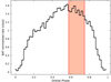 |
Fig. 1. Swift/BAT folded light curve of OAO 1657-415 using 50 phase bins, an orbital period of 10.45 days, and a reference epoch of 52298.01 MJD (Jenke et al. 2012). The vertical orange region corresponds to the NuSTAR observation used in this paper. The NuSTAR observation spans ∼17% of the orbit of OAO 1657-415, starting on phase 0.576. |
3. Results
3.1. Timing analysis
In Fig. 2 we show a light curve of the source with a binning of ten times the pulsar period (370 s) in the 3–79 keV energy range. Different variability patterns can be seen, that is, non-statistical changes in count rate, ranging from a few hundred seconds to several kiloseconds, with intensity increasing by up to five times. We identify four time periods (shown with different colours in Fig. 2) that we refer to from here on as intervals I, II, III, and IV.
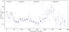 |
Fig. 2. Background-corrected light curve of OAO 1657-415 with a binning of 370 s, starting at 58645.5355 MJD. The light curve was further subdivided into four intervals (colour coded) in order to make a timing and spectral analysis. |
Light curves were extracted in different energy ranges associated with each interval: 3–15 keV, 15–30 keV, 30–50 keV, and 50–79 keV, respectively. Using the powspec task, we extracted power spectra associated with each interval. Figure 3 shows the power spectra associated with the complete observation, where the fundamental pulse and seven harmonics are identified. Features in the power spectra of intervals I to IV are similar to those of the complete observation.
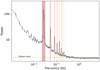 |
Fig. 3. Power spectra associated with the complete observation. The fundamental pulse and harmonics are highlighted with different colours. The same features are seen in the power spectra of the individual intervals. Spectra were normalised using Leahy’s normalisation. |
The efsearch task was used to estimate the best period associated to each fundamental pulse present in each interval. The period and uncertainties were estimated by performing 1000 simulations for each light curve using the observed count statistics, as described in Boldin et al. (2013). In Table 1 we present the best period and uncertainties derived from the mentioned procedure for each interval. There is a decay in the pulse throughout the observation, which is possibly due to a Doppler shift in the NS spin before the eclipse, which is similar to findings by Fogantini et al. (2021). This change in frequency is given by the following equation (Gong 2005):
 (1)
(1)
Best periods and uncertainties for each time interval derived from the algorithm described in Boldin et al. (2013).
where x is the projected semi-major axis (x = apsin(i)/c), K is semi-amplitude, e is the eccentricity, and Pb is the orbital period of the binary system. Taking the orbital ephemeris from Jenke et al. (2012), we obtain ΔP = 1/Δν ≈ 0.1 s. This equation returns the average change in frequency along the whole orbit. As the exposure time of the NuSTAR observation occupies ∼17% of the orbital period. On first approximation, we can weight the total average frequency change by the observed fraction. If we multiply by a factor 0.17 we get a value of ∼0.017 s variation, which provides an explanation for the period shifts given by the orbital Doppler effect.
With the efold task, we proceeded to fold light curves associated to each interval in different energy ranges. Figure 4 shows an example of this for interval I; the other intervals are similar. This analysis shows that pulses are detected up to the last defined interval associated with the maximum energy allowed by NuSTAR. It is probable that pulses are detected above 79 keV in all periods as already reported using INTEGRAL observations (Barnstedt et al. 2008).
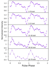 |
Fig. 4. Background-corrected energy-resolved pulse profiles for interval I. Profiles were folded with the best period found using efsearch. The NS spin period modulation is detected at all the energy bands. |
Light curves were also extracted for the complete observation at energy ranges: soft: 3–15 keV and hard: 15–50 keV. Figure 5 shows the hardness ratio obtained from these ranges. As can be seen, the brightness variations are followed by changes in the hardness ratio.
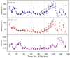 |
Fig. 5. NuSTAR light curve with 370s bin size. Each plot contains three panels: soft (upper panel) and hard (middle panel) light curves, and hardness ratio (lower panel). |
3.2. Spectral analysis
In order to characterise the spectrum of the source, we performed a spatially resolved spectral analysis, where the source and background were modelled simultaneously using the two NuSTAR detectors. A calibration constant was included which varies the FPMA and FPMB spectra by 2%. The source broad-band spectrum in NS-HMXBs has a relatively complicated shape and can be appropriately fitted by a composite model with two continuum components: blackbody emission with the kT at low energies, and a power law with an exponential cut-off at high energies. In particular, for OAO 1657−415, the spectrum was fitted using different models for the high-energy component: highecut, bknpow, cutoffpl, and comptt (Titarchuk 1994). After several tests, we found that the best fit is consistent with a cutoffpl. For the lower energy component we tested the bbody and diskbb models (Mitsuda et al. 1984). This ensures that the emission comes from the NS or the accretion disk. The best fit was obtained with a bbody at ∼0.2 keV. The interstellar absorption was modelled using the Tuebingen-Boulder interstellar absorption model (tbabs), with solar abundances set according to Wilms et al. (2000), and the effective cross-sections given by Verner et al. (1996). Two emission lines are present at ∼6.4 keV and ∼7 keV (Audley et al. 2000; Chakrabarty et al. 2002). The Kβ emission line width was left frozen to the best fit value. The final model results in a χ2/d.o.f.: 2434.83/2249.
We included a Lorentzian cyclotron line component cyclabs to the model (Mihara et al. 1990; Makishima et al. 1990). A count flux deficit can be seen around ∼35 keV (see Fig. 6) if we fix the depth to zero. We obtain a very large value for the cyclotron line width of σcyc ∼ 25 keV, which is statistically equal to the value obtained by Orlandini et al. (1999) using Beppo-SAX observations. For subsequent fits we left the line width fixed at 10 keV. This is consistent with the correlation between the width and the energy centroid of the cyclotron lines for different X-ray binaries (Staubert et al. 2020). The final fit gives χ2/d.o.f.: 2398.51/2247, which is significantly better than the model without the cyclotron absorption component.
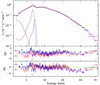 |
Fig. 6. Top panel: NuSTAR’s FPMA and FPMB average energy spectrum for OAO 1657-415. The continuum can be described by contributions of an absorbed cut-off power law and a blackbody. Gaussian distributions were used to model emission lines seen at ∼6.4 keV and ∼7 keV. Middle panel: residuals associated with the continuum model. Bottom panel: residuals associated with the continuous model plus cyclabs with depth equal to zero. A clear count flux deficit can be seen at around ∼35 keV. |
Final model parameters and uncertainties are listed in Table 2. The cutoffpl normalisation reported is in units of photons keV−1 cm−2 s−1 at 1 keV. The blackbody normalisation reported is in units of  where L39 is the source luminosity in units of 1039 erg s−1 and D10 is the distance to the source in units of 10 kpc. The Gaussian normalisations reported are in units of total photons cm−2 s−1 in the line. The equivalent widths of the Kα and Kβ emission lines are 0.257 ± 0.01 keV and 0.0248 ± 0.009 keV respectively. Jaisawal et al. (2021) reports an equivalent width of 1 keV. This value does not differ from the one found here, as it is poorly constrained, and depends on the observation and segments considered. The unabsorbed flux was computed using the cflux convolution model, yielding 1.17 × 10⁻⁹ erg cm−2 s−1 in the 3–79 keV energy range for the total continuum spectrum and the emission lines inclusively.
Final parameters of the average energy spectrum associated with the described models.
To analyse the spectral characteristics of each time interval, the spectra associated with these were extracted. The four periods were described with a cutoffpl+bbody model for the continuum and two Gaussian distributions to account for the Fe emission lines. In addition, a Lorentzian cyclotron line component was included in three of the four intervals. Interval III could not be correctly fitted with the addition of the cyclotron component, and so the centroid energy line had to be fixed at best fit, which was ∼34 keV. The final model parameters for each interval are listed in Table 3, and their associated spectra are shown in Fig. 7. The centroid energy Ecyc can vary between 31.3 keV and 38.2 keV.
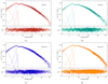 |
Fig. 7. Time-resolved spectra for each defined interval fitted with Model bbody+cutoffpl+gauss plus cyclabs. Bottom panel: each subplot indicates the model residuals. |
Parameters associated with the models in different time intervals.
To test the significance of the cyclotron absorption line we use the F-test routine in XSPEC by comparing the model bbody+cutoffpl+gauss with the same model but with the additional cyclotron absorption line. This results in an F-statistic of 17.01 and a probability of 4.6 × 10⁻⁸. However, this analysis is not correct for the detection of multiplicative components or absorption/emission lines (Orlandini et al. 1999; Protassov et al. 2002). It was decided that another strategy be used: simulations were performed with the fake-it task of xspec. The line energy and depth were adjusted, leaving fixed width at 10 keV. With this, we drew 5 × 10⁴ sampled spectra with identical model and continuum parameters, and then counted how many of the sampled spectra had a depth greater than that of the adjusted line of the real spectra. The ratio, r, between the latter number and the total sampled spectra gives an estimate of the probability of obtaining a greater depth than the actual spectra simply by chance. The lower this ratio, the more confidently we can assume the genuine presence of a cyclotron absorption line. The results of this evaluation for the total observation and each time interval chosen are presented in Table 4. We note that the presence of the line decreases with the passage of observation time. This is to be expected as the NS is eclipsed. We consider the presence of the cyclotron line to be significant in intervals I and II with a significance of 99.96% and 97.67%, respectively. For intervals III and IV, we consider that the presence is not significant. It is unusual that the width of the absorption line is very large since the range of widths in the literature varies from 0 to 15 keV. Only in Orlandini et al. (1999) is the width of the absorption line reported to be larger than what is found in the literature. We consider that the absorption line is weak, and therefore the width is affected by this. This weak component of the line can be reflected in the large errors associated with the width and its decreasing depth over time.
Cyclotron absorption line significance, σcyc = 1 − r, for each time interval.
The obtained differences in the model parameters between intervals are typical for NS-HMXBs (i.e. Ding et al. 2021). These differences give us information about the relationship between the geometry of the pulsar beam and the magnetic field (Maitra 2017).
4. Discussion
Figure 8 shows the folded light curves associated with each time interval in the 3–79 keV energy range. These were obtained using light curves folded at the intervals shown in Table 1. The epoch for all pulsations was defined as 58645.5 MJD in order to be able to compare them. As can be seen, all the pulsations are out of phase. The observed phase shift is due to the different pulse periods adopted for the epoch folding in each interval. Different time folding using the same epoch but different pulses introduces a false pulse phase shift:
 (2)
(2)
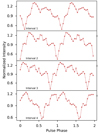 |
Fig. 8. Background-corrected pulse profiles associated with each interval folded with the best periods found (see Table 1). |
where Δt is the time distance between the midpoints of the two time intervals and ΔP is the difference in length between the two periods. The phase shift of the pulses observed in Fig. 8 is compatible with the formula above. The pulsations of intervals I, II, and III are similar to each other. The pulse in interval IV is the most unusual; it also has a lower intensity than the other pulsations. Moreover, the spectral index in interval IV drops noticeably by half with respect to interval III. This is accompanied by a change in the hardness ratio diagram, as shown in Fig. 5. Also, the light curve of interval IV presents a flare feature.
4.1. Cyclotron resonant scattering features
Cyclotron resonant scattering features (CRSFs) or cyclotron absorption lines are produced near the magnetic poles of an accreting NS. Electrons move perpendicularly to the magnetic field lines, assuming discrete energy levels referred to as Landau levels. Resonance features are generated when photons are scattered by electrons at resonance energy, which is commonly seen in the X-ray spectrum as a deficit in the continuum flux at energies between 10 and 80 keV (Jaisawal & Naik 2017). The energy of the fundamental level corresponds to the energy gap between two adjacent Landau levels. The detection of this line can be used to estimate the dipolar surface magnetic field of a pulsar (Christodoulou et al. 2018):
 (3)
(3)
Using Ecyc = 35.6 ± 2.5 keV as the fundamental energy (n = 1), and assuming a canonical gravitational redshift for the NS of zg = 0.306 (Christodoulou et al. 2019), we estimate a dipolar surface magnetic field of Bcyc ≈ 4.0 ± 0.2 × 10¹² G, consistent with other NS-HMXB sources (Jaisawal & Naik 2017; Staubert et al. 2019).
4.2. Distance to OAO 1657-415
From the derived dipolar magnetic field intensity, we can estimate the distance to OAO 1657-415 through the equation (Cui 1997):
where Fx is the minimum bolometric X-ray flux at which the X-ray pulsations are still detectable. In our case, we get 1.17 ± 0.01 × 10⁻⁹ erg cm−2 s−1, in the 3–79 keV energy range. Assuming a NS mass of 1.8 ± 0.3 M⊙ (Falanga et al. 2015), a standard radius of 10 km, and a spin period P of 37.03 ± 0.01 s, we obtain an approximate distance to OAO 1657-415 of 1.05 ± 0.08 kpc. This method is not as accurate as others, given that the error in Fx can be significant, leading to an error on the distance much larger than indicated, see the explanation of the source location in the Corbet diagram for a possible explanation of flux variation (see Fig. 9). Also, Fx may not be the minimum bolometric X-ray flux. Barnstedt et al. (2008) analysed energy-resolved pulse profiles using INTEGRAL observations, where the authors note that the pulses are detected in the 120–160 keV energy range. We take Fx obtained in this work as an approximate upper limit. Therefore, we consider this value to be a rough lower limit compared to distances already established with other methods. The distance obtained with Gaia based on ultra-precise angular parallaxes of the optical companion, which is  kpc, is consistent with the value obtained by this method (Malacaria et al. 2020). Mason et al. (2009) report a distance using a luminosity range between 1.5 × 1036 erg s−1 and 1037 erg s−1. The lower limit is compatible with the distance obtained with Gaia, and therefore with the rough lower limit reported in this work.
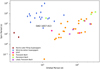 |
Fig. 9. Corbet diagram for the different population of NS-HMXB with measured Porb and Pspin periods. Brown diamonds represent the Roche-lobe-filling supergiant systems. Blue diamonds represent the wind-accretion supergiant systems. Pink dots represent the SFXTs. Orange dots represent the transients Be/X systems while green crosses represent the persistent Be/X systems. The violet crosses represent the transient Be/X candidates. Diagram adapted from Jenke et al. (2012). |
4.3. Possible weak dependence between luminosity and the CRSF
In systems where a cyclotron absorption line appears there may be a positive or negative correlation between cyclotron line energy Ecyc and X-ray luminosity (Kretschmar et al. 2019). In order to check the statistical significance of such a relationship in the NuSTAR data, we used the average unabsorbed luminosity and the unabsorbed luminosities associated with each interval, assuming a distance to the source of  kpc (Malacaria et al. 2020). The average 3–79 keV unabsorbed luminosity is ∼6.81 × 1035erg s−1. The unabsorbed luminosities associated with each interval are listed in Table 5. If we exclude interval IV, we find a positive correlation with a Pearson r2 coefficient of ∼0.8, with a p-value of 0.416, which is high as it arises from a small population. However, if interval IV is taken into account then the Pearson correlation coefficient is ∼0.52. In both cases we find a relationship with a positive r2. Similarly, Bahal et al. (2019) reported a weak relationship between these two variables.
Estimated cyclotron line energies from spectral fits in units of keV.
4.4. OAO 1657-415 in the Corbet diagram
The HMXBs can be classified as Roche lobe-filling supergiants, wind accretion supergiants, and Be-HMXBs, with these latter being found in large numbers (Liu et al. 2006; Chaty 2013).
The Corbet diagram compares the orbital period to the spin period of the accreting pulsar (Corbet 1984, 1986). This can be interpreted as a ‘tidal’ lock between the rotational velocity of the magnetospheric radius and the Keplerian velocity, i.e. the equilibrium period. For short spin periods, matter cannot be accretted due to the propeller mechanism (Illarionov & Sunyaev 1975). For spin periods longer than the equilibrium period, matter can be accreted onto the pulsar, thus reducing the angular momentum and hence the spin period.
The values of the spin and orbital periods of OAO 1657-415 put it in an interesting position in the Corbet diagram; in between three types of sources: wind accretion systems, Roche lobe overflow systems, and Be X-ray binaries (Chakrabarty et al. 1993) (see Fig. 9). Its position in the Corbet diagram is related to its spectral type: Ofpe/WNL. These stars exhibit slower wind velocities and higher mass-loss rates (Martins et al. 2007). The combination of these characteristics allows for a higher accretion rate, which drives a transfer of angular momentum to the pulsar (Mason et al. 2009). This spectral type occurs at the transition of main sequence OB stars and hydrogen-depleted Wolf-Rayet stars. Humphreys & Davidson (1994) proposed that this spectral type is the hot quiescent state of the luminous blue variables stars (LBVs). This could explain the significant X-ray luminosity variability over months, as it would increase the mass-loss rate or stellar radius, generating a closer approach to the Roche lobe and therefore increasing the mass-transfer rate (see Kuulkers et al. 2007).
5. Conclusions
In this work we analyse the spectral and timing properties of OAO 1657-415 observed by the NuSTAR observatory on June 10, 2019, during the brightest orbital phase. We also included the Swift/BAT cumulative light curve spanning ∼16 years. The NuSTAR light curve was divided into four intervals in order to characterise each spectral period. Power spectra were extracted for each interval, detecting the NS spin period (pulse) in all of them. At the same time, different light curves were taken in different energy ranges in order to analyse the extent to which the pulse was detected. We find that the pulse is detected up to ∼80 keV in all time intervals.
The spectrum of OAO 1657-415 can be approximately described by a power law with an exponential cut-off. The Comptonisation of soft X-rays above the surface of the NS can explain the continuum emission. Iron Kα and Kβ emission lines are present in the spectra. No emission lines associated with ionised material were detected (Pradhan et al. 2014), which is probably due to the low to moderate spectral resolution of NuSTAR. At the same time, a flux deficit at around 35 keV was observed in the residual spectrum. This indicates the presence of a cyclotron absorption feature. An absorption model was included, resulting in a better fit than the continuum and emission lines only. We found that the cyclotron absorption line has a significance of ∼3.4σ. This absorption line coincides with one found by Orlandini et al. (1999) detected with Beppo-SAX. We interpret this second finding as evidence of the presence of this absorption feature on the X-ray spectra of OAO 1657-415.
By obtaining the energy centroid of the absorption line, the magnetic field on the surface of the NS was estimated to be 4.0 ± 0.2 × 10¹² G. By combining the magnetic field and the X-ray flux, we get a lower limit on the estimated distance of ≳1 kpc. This distance is compatible with the distance obtained from Gaia observations, and in turn from near-infrared observations estimated by Mason et al. (2009). As already seen in other sources, we find a possible positive relationship between the cyclotron energy and the X-ray luminosity. Finally, we mention the striking position of OAO 1657-415 in the Corbet diagram. This position can be attributed to its spectral type, which also explains the significant variability in its X-ray luminosity.
Acknowledgments
We thank the anonymous reviewer for their valuable comments on this manuscript. FAF, JAC and FG acknowledge support by PIP 0113 (CONICET). FAF is fellow of CONICET. JAC and FG are CONICET researchers. This work received financial support from PICT-2017-2865 (ANPCyT). This work was partly supported by the Centre National d’Etudes Spatiales (CNES), and based on observations obtained with MINE: the Multi-wavelength INTEGRAL NEtwork. JAC was also supported by grant PID2019-105510GB-C32/AEI/10.13039/501100011033 from the Agencia Estatal de Investigación of the Spanish Ministerio de Ciencia, Innovación y Universidades, and by Consejería de Economía, Innovación, Ciencia y Empleo of Junta de Andalucía as research group FQM-322, as well as FEDER funds.
References
- Arnaud, K. A. 1996, in Astronomical Data Analysis Software and Systems V, eds. G. H. Jacoby, & J. Barnes, ASP Conf. Ser., 101, 17 [NASA ADS] [Google Scholar]
- Audley, M. D., Nagase, F., Mitsuda, K., Angelini, L., & Kelley, R. L. 2000, Am. Astron. Soc. Meeting Abstracts, 197, 84.05 [NASA ADS] [Google Scholar]
- Bahal, V., Pradhan, P., Maitra, C., Raichur, H., & Paul, B. 2019, ApJ, submitted [arXiv:1906.02917] [Google Scholar]
- Barnstedt, J., Staubert, R., Santangelo, A., et al. 2008, A&A, 486, 293 [NASA ADS] [CrossRef] [EDP Sciences] [Google Scholar]
- Boldin, P. A., Tsygankov, S. S., & Lutovinov, A. A. 2013, Astron. Lett., 39, 375 [NASA ADS] [CrossRef] [Google Scholar]
- Chakrabarty, D., Grunsfeld, J. M., Prince, T. A., et al. 1993, ApJ, 403, L33 [CrossRef] [Google Scholar]
- Chakrabarty, D., Wang, Z., Juett, A. M., Lee, J. C., & Roche, P. 2002, ApJ, 573, 789 [NASA ADS] [CrossRef] [Google Scholar]
- Chaty, S. 2013, Adv. Space Res., 52, 2132 [NASA ADS] [CrossRef] [Google Scholar]
- Christodoulou, D. M., Laycock, S. G. T., Kazanas, D., & Contopoulos, I. 2018, Res. Astron. Astrophys., 18, 142 [Google Scholar]
- Christodoulou, D. M., Laycock, S. G. T., & Kazanas, D. 2019, Res. Astron. Astrophys., 19, 146 [Google Scholar]
- Corbet, R. H. D. 1984, A&A, 141, 91 [NASA ADS] [Google Scholar]
- Corbet, R. H. D. 1986, MNRAS, 220, 1047 [NASA ADS] [CrossRef] [Google Scholar]
- Cui, W. 1997, ApJ, 482, L163 [NASA ADS] [CrossRef] [Google Scholar]
- Ding, Y. Z., Wang, W., Epili, P. R., et al. 2021, MNRAS, 506, 2712 [NASA ADS] [CrossRef] [Google Scholar]
- Falanga, M., Bozzo, E., Lutovinov, A., et al. 2015, A&A, 577, A130 [NASA ADS] [CrossRef] [EDP Sciences] [Google Scholar]
- Fogantini, F. A., García, F., Combi, J. A., & Chaty, S. 2021, A&A, 647, A75 [NASA ADS] [CrossRef] [EDP Sciences] [Google Scholar]
- Fortin, F., Chaty, S., & Sander, A. 2020, ApJ, 894, 86 [NASA ADS] [CrossRef] [Google Scholar]
- Gaia Collaboration (Brown, A. G. A., et al.) 2018, A&A, 616, A1 [NASA ADS] [CrossRef] [EDP Sciences] [Google Scholar]
- García, F., Fogantini, F. A., Chaty, S., & Combi, J. A. 2018, A&A, 618, A61 [NASA ADS] [CrossRef] [EDP Sciences] [Google Scholar]
- Gong, B. 2005, Phys. Rev. Lett., 95, 261101 [NASA ADS] [CrossRef] [Google Scholar]
- Harrison, F. A., Craig, W. W., Christensen, F. E., et al. 2013, ApJ, 770, 103 [Google Scholar]
- Humphreys, R. M., & Davidson, K. 1994, PASP, 106, 1025 [NASA ADS] [CrossRef] [Google Scholar]
- Illarionov, A. F., & Sunyaev, R. A. 1975, A&A, 39, 185 [NASA ADS] [Google Scholar]
- Jaisawal, G. K., & Naik, S. 2014, Bull. Astron. Soc. India, 42, 147 [NASA ADS] [Google Scholar]
- Jaisawal, G. K., & Naik, S. 2017, in 7 years of MAXI: monitoring X-ray Transients, eds. M. Serino, M. Shidatsu, W. Iwakiri, & T. Mihara, 153 [Google Scholar]
- Jaisawal, G. K., Naik, S., Epili, P. R., et al. 2021, JApA, 42, 72 [NASA ADS] [Google Scholar]
- Jenke, P. A., Finger, M. H., Wilson-Hodge, C. A., & Camero-Arranz, A. 2012, ApJ, 759, 124 [NASA ADS] [CrossRef] [Google Scholar]
- Kretschmar, P., Fürst, F., Sidoli, L., et al. 2019, New Astron. Rev., 86, 101546 [Google Scholar]
- Kuulkers, E., Shaw, S. E., Paizis, A., et al. 2007, A&A, 466, 595 [NASA ADS] [CrossRef] [EDP Sciences] [Google Scholar]
- Liu, Q. Z., van Paradijs, J., & van den Heuvel, E. P. J. 2006, A&A, 455, 1165 [NASA ADS] [CrossRef] [EDP Sciences] [Google Scholar]
- Maitra, C. 2017, JApA, 38, 50 [NASA ADS] [Google Scholar]
- Makishima, K., Mihara, T., Ishida, M., et al. 1990, ApJ, 365, L59 [NASA ADS] [CrossRef] [Google Scholar]
- Malacaria, C., Jenke, P., Roberts, O. J., et al. 2020, ApJ, 896, 90 [NASA ADS] [CrossRef] [Google Scholar]
- Martins, F., Genzel, R., Eisenhauer, F., et al. 2007, Highlights Astron., 14, 207 [NASA ADS] [Google Scholar]
- Mason, A. B., Clark, J. S., Norton, A. J., Negueruela, I., & Roche, P. 2009, A&A, 505, 281 [NASA ADS] [CrossRef] [EDP Sciences] [Google Scholar]
- Mason, A. B., Clark, J. S., Norton, A. J., et al. 2012, MNRAS, 422, 199 [NASA ADS] [CrossRef] [Google Scholar]
- Mihara, T., Makishima, K., Ohashi, T., Sakao, T., & Tashiro, M. 1990, Nature, 346, 250 [NASA ADS] [CrossRef] [Google Scholar]
- Mitsuda, K., Inoue, H., Koyama, K., et al. 1984, PASJ, 36, 741 [NASA ADS] [Google Scholar]
- Negueruela, I., Smith, D. M., Reig, P., Chaty, S., & Torrejón, J. M. 2006, in The X-ray Universe 2005, ed. A. Wilson, ESA Spec. Publ., 604, 165 [NASA ADS] [Google Scholar]
- Orlandini, M., dal Fiume, D., del Sordo, S., et al. 1999, A&A, 349, L9 [NASA ADS] [Google Scholar]
- Parmar, A. N., Branduardi-Raymont, G., Pollard, G. S. G., et al. 1980, MNRAS, 193, 49P [NASA ADS] [CrossRef] [Google Scholar]
- Polidan, R. S., Pollard, G. S. G., Sanford, P. W., & Locke, M. C. 1978, Nature, 275, 296 [NASA ADS] [CrossRef] [Google Scholar]
- Pradhan, P., Maitra, C., Paul, B., Islam, N., & Paul, B. C. 2014, MNRAS, 442, 2691 [Google Scholar]
- Pradhan, P., Raman, G., & Paul, B. 2019, MNRAS, 483, 5687 [NASA ADS] [CrossRef] [Google Scholar]
- Protassov, R., van Dyk, D. A., Connors, A., Kashyap, V. L., & Siemiginowska, A. 2002, ApJ, 571, 545 [NASA ADS] [CrossRef] [Google Scholar]
- Schwarm, F. W., Schönherr, G., Falkner, S., et al. 2017, A&A, 597, A3 [NASA ADS] [CrossRef] [EDP Sciences] [Google Scholar]
- Staubert, R., Trümper, J., Kendziorra, E., et al. 2019, A&A, 622, A61 [NASA ADS] [CrossRef] [EDP Sciences] [Google Scholar]
- Staubert, R., Ducci, L., Ji, L., et al. 2020, A&A, 642, A196 [NASA ADS] [CrossRef] [EDP Sciences] [Google Scholar]
- Titarchuk, L. 1994, ApJ, 434, 570 [NASA ADS] [CrossRef] [Google Scholar]
- Verner, D. A., Ferland, G. J., Korista, K. T., & Yakovlev, D. G. 1996, ApJ, 465, 487 [Google Scholar]
- Wilms, J., Allen, A., & McCray, R. 2000, ApJ, 542, 914 [Google Scholar]
All Tables
Best periods and uncertainties for each time interval derived from the algorithm described in Boldin et al. (2013).
Final parameters of the average energy spectrum associated with the described models.
All Figures
|
Fig. 1. Swift/BAT folded light curve of OAO 1657-415 using 50 phase bins, an orbital period of 10.45 days, and a reference epoch of 52298.01 MJD (Jenke et al. 2012). The vertical orange region corresponds to the NuSTAR observation used in this paper. The NuSTAR observation spans ∼17% of the orbit of OAO 1657-415, starting on phase 0.576. |
| In the text | |
|
Fig. 2. Background-corrected light curve of OAO 1657-415 with a binning of 370 s, starting at 58645.5355 MJD. The light curve was further subdivided into four intervals (colour coded) in order to make a timing and spectral analysis. |
| In the text | |
|
Fig. 3. Power spectra associated with the complete observation. The fundamental pulse and harmonics are highlighted with different colours. The same features are seen in the power spectra of the individual intervals. Spectra were normalised using Leahy’s normalisation. |
| In the text | |
|
Fig. 4. Background-corrected energy-resolved pulse profiles for interval I. Profiles were folded with the best period found using efsearch. The NS spin period modulation is detected at all the energy bands. |
| In the text | |
|
Fig. 5. NuSTAR light curve with 370s bin size. Each plot contains three panels: soft (upper panel) and hard (middle panel) light curves, and hardness ratio (lower panel). |
| In the text | |
|
Fig. 6. Top panel: NuSTAR’s FPMA and FPMB average energy spectrum for OAO 1657-415. The continuum can be described by contributions of an absorbed cut-off power law and a blackbody. Gaussian distributions were used to model emission lines seen at ∼6.4 keV and ∼7 keV. Middle panel: residuals associated with the continuum model. Bottom panel: residuals associated with the continuous model plus cyclabs with depth equal to zero. A clear count flux deficit can be seen at around ∼35 keV. |
| In the text | |
|
Fig. 7. Time-resolved spectra for each defined interval fitted with Model bbody+cutoffpl+gauss plus cyclabs. Bottom panel: each subplot indicates the model residuals. |
| In the text | |
|
Fig. 8. Background-corrected pulse profiles associated with each interval folded with the best periods found (see Table 1). |
| In the text | |
|
Fig. 9. Corbet diagram for the different population of NS-HMXB with measured Porb and Pspin periods. Brown diamonds represent the Roche-lobe-filling supergiant systems. Blue diamonds represent the wind-accretion supergiant systems. Pink dots represent the SFXTs. Orange dots represent the transients Be/X systems while green crosses represent the persistent Be/X systems. The violet crosses represent the transient Be/X candidates. Diagram adapted from Jenke et al. (2012). |
| In the text | |
Current usage metrics show cumulative count of Article Views (full-text article views including HTML views, PDF and ePub downloads, according to the available data) and Abstracts Views on Vision4Press platform.
Data correspond to usage on the plateform after 2015. The current usage metrics is available 48-96 hours after online publication and is updated daily on week days.
Initial download of the metrics may take a while.