| Issue |
A&A
Volume 658, February 2022
|
|
|---|---|---|
| Article Number | A199 | |
| Number of page(s) | 10 | |
| Section | Galactic structure, stellar clusters and populations | |
| DOI | https://doi.org/10.1051/0004-6361/202140921 | |
| Published online | 24 February 2022 | |
Hot Jupiters, cold kinematics
High phase space densities of host stars reflect an age bias
1
Lund Observatory, Department of Astronomy and Theoretical Physics, Lund University, Box 43 221 00 Lund, Sweden
e-mail: This email address is being protected from spambots. You need JavaScript enabled to view it.
2
Centre for Mathematical Sciences, Lund University, Box 118 221 00 Lund, Sweden
Received:
29
March
2021
Accepted:
24
November
2021
Abstract
Context. The birth environments of planetary systems are thought to influence planet formation and orbital evolution through external photoevaporation and stellar flybys. Recent work has claimed observational support for this, in the form of a correlation between the properties of planetary systems and the local Galactic phase space density of the host star. In particular, hot Jupiters are overwhelmingly present around stars in regions of high phase space density, which may reflect a formation environment with high stellar density.
Aims. We aim to investigate whether the high phase space density may have a Galactic kinematic origin: hot Jupiter hosts may be biased towards being young and therefore kinematically cold, because tidal inspiral leads to the destruction of the planets on gigayear timescales, and the velocity dispersion of stars in the Galaxy increases on similar timescales.
Methods. We used 6D positions and kinematics from Gaia for the hot Jupiter hosts and their neighbours, and we constructed distributions of the phase space density. We investigated correlations between the stars’ local phase space density and peculiar velocity.
Results. We find a strong anti-correlation between the phase space density and the host star’s peculiar velocity with respect to the Local Standard of Rest. Therefore, most stars in ‘high-density’ regions are kinematically cold, which may be caused by the aforementioned bias towards detecting hot Jupiters around young stars before the planets’ tidal destruction.
Conclusions. We do not find evidence in the data for hot Jupiter hosts preferentially being in phase space overdensities compared to other stars of similar kinematics, nor therefore for their originating in birth environments of high stellar density.
Key words: planetary systems / open clusters and associations: general / planet-star interactions / stars: kinematics and dynamics / Galaxy: disk / solar neighborhood
© ESO 2022
1. Introduction
The birth environment of a planetary system, that is, the size and density of the stellar cluster or association where the system forms, is thought to have an impact on the nature of the planetary system. This can occur through external photoevaporation of the protoplanetary disc and/or through stellar flybys truncating the disc or perturbing formed systems (de La Fuente Marcos & de La Fuente Marcos 1997; Laughlin & Adams 1998; Adams et al. 2006; Malmberg et al. 2007a; Winter et al. 2018; Li et al. 2019, 2020a,b). Direct evidence of the impact of birth environments on planetary system formation is hard to obtain, because of the low number (in absolute terms) of planets found in clusters compared to the field, and the challenges of detecting planets around young stars. Winter et al. (2020, henceforth W20) recently proposed an ingenious way around this using the local phase space density (the density of nearby stars in the 6D phase space of Galactic position and velocity) of an exoplanet host star as a proxy for the crowdedness of its birth environment. By assuming that the current density reflects the past density at birth, W20 could look for correlations between this density and the properties of planetary systems.
One of the most significant results from W20 was that the host stars of hot Jupiters are nearly always in high-density regions of phase space. This is naturally explained if the primary migration channel for hot Jupiters is dynamical excitation through planet–planet scattering and/or Lidov–Kozai cycles, followed by tidal dissipation (Rasio & Ford 1996; Weidenschilling & Marzari 1996; Wu & Murray 2003; Fabrycky & Tremaine 2007). Here, the external dynamical perturbations in a dense birth environment would provide the trigger for this high-eccentricity migration to begin (Malmberg et al. 2007b, 2011; Parker & Goodwin 2009; Parker & Quanz 2012; Brucalassi et al. 2016; Rodet et al. 2021). Disc migration offers an alternative channel to produce hot Jupiters (Lin et al. 1996), which might also be affected by the environment through photoevaporation of the protoplanetary disc (Winter et al. 2018).
This interpretation of W20’s finding, however, relies on the assumption that a high local phase space density for a star at the present time reflects a high density of its formation environment. Here, we examine this assumption. In Hamiltonian mechanics, Liouville’s Theorem indeed states that phase space density is constant along trajectories, implying it would be inherited from a star’s formation site. Yet, this does not apply to stars in the Galaxy on gigayear timescales, because the Galactic potential is not time-independent, and the dynamics are not completely collisionless, violating the conditions for Liouville’s Theorem to hold. In particular, stellar populations are ‘heated’ with age and increase their velocity dispersion and vertical scale height, through interactions with giant molecular clouds and spiral arms (Spitzer & Schwarzschild 1951; Wielen 1977; De Simone et al. 2004; Nordström et al. 2004). Numerical simulations (Kamdar et al. 2019a,b) find that the imprint of a birth cluster, in comoving conatal pairs and phase space overdensities, largely disappear after ∼1 Gyr. Hence, it is not clear that the foundational assumption of W20 holds. Instead, it is possible that a star’s phase space density reflects coarser features of Galactic structure and kinematics, such as disc heating with age, or the existence of a Galactic thick disc of larger scale height than the thin disc to which the Sun belongs (Gilmore & Reid 1983), rather than the nature of the birth cluster. While noting that Galactic dynamics could play a role in determining the phase space density, W20 interpreted their results in the context of the birth environment hypothesis.
Here we show that, in general, the majority of stars that are currently in high-density regions of phase space as defined by W20 simply have cold kinematics in the Galactic disc: near-circular orbits and little vertical motion. The high-density classification thus relates to the lower average age and lesser kinematic heating of the stars, and not to a memory of their birth environment.
2. Methods: Mahalanobis distance and description of the phase space density distribution
We followed W20 in using the Mahalanobis distance (Mahalanobis 1936) in 6D phase space to construct the phase space density. This is essentially a reoriented and stretched Euclidean metric, represented by the quadratic form
 (1)
(1)
where x1 and x2 are two (6D) phase space positions and C is the 6 × 6 covariance matrix of the whole sample:
 (2)
(2)
for i, j = 1…6, where ⟨⋯⟩ denotes the mean. It has the advantage of defining a distance in a space whose dimensions have different dynamic ranges and different physical dimensions. However, as it returns a rescaled, dimensionless quantity, its physical interpretation is not obvious. We will therefore relate the density derived from this metric to the host stars’ corresponding physical quantities, especially the peculiar velocity: the star’s velocity with respect to that of a circular orbit in the Galactic plane (the Local Standard of Rest).
To begin, we followed W20 as closely as possible to ensure a direct comparison with their work. For each target star, we first queried all objects in Gaia Data Release 2 (DR2) or Early Data Release 3 (EDR3; Gaia Collaboration 2016, 2018, 2021a) within 80 pc of the target. The criterion for inclusion was that the star possess a radial velocity measured by Gaia as well as a positive parallax. We then converted the astrometric, positional, and RV information from Gaia to a heliocentric Cartesian position and velocity. The distance was obtained by inverting the parallax. A velocity correction from the heliocentric rest frame to the Local Standard of Rest (the velocity of a body on a circular orbit at the Sun’s position in the Galaxy) from Schönrich et al. (2010) was then applied: (U, V, W)⊙ = (11.1, 12.24, 7.25) km s−1.
We then defined the Mahalanobis metric on the sample using the covariance matrix of the positions and velocities of all stars within 80 pc of the target. For stars with at least 400 neighbours within 40 pc, we randomly chose up to 600 such neighbours. For each of these, as well as the target, we found the 20th nearest neighbour by the Mahalanobis distance dM, 20 and used this to define the local 6D phase space density  . We then normalised ρ20 so that the median of the distribution is 1. Next, we fitted a two-component Gaussian mixture model to the distribution of the logarithm of the rescaled density. Outliers greater than two standard deviations from the mean, or with densities ρ20 > 50, were clipped before fitting the model. We removed systems where a one-component model is a good fit to the density distribution (p > 0.05 on a KS test); three such systems were removed. Finally, we calculated the probability that the target star was drawn from the high-density or the low-density component of the Gaussian mixture model. If ρ > 50, we assigned it to the high-density population.
After this, W20 analysed differences between the high-density population (Phigh > 0.84) and the low-density population (Phigh < 0.16). The power of this approach is illustrated in Fig. 1, where we show the semi-major axes and eccentricities of known exoplanets1 whose hosts were cross-matched to Gaia EDR3 and whose masses and ages are between 0.7 − 2.0 M⊙ and 1.0 − 4.5 Gyr, respectively (as in W20). As W20, we see noticeable differences between the distributions of planets orbiting high-density and low-density hosts. In this paper, we focus on the overabundance of hot Jupiters orbiting the high-density hosts: the ratio of hot-to-cold Jupiter hosts is 1.4 for the high-density hosts and only 0.4 for the low-density hosts (in this paper, following W20, we defined hot Jupiters as planets with a mass M > 50 M⊕ and a semi-major axis a < 0.2 au, and cold Jupiters as planets with a mass M > 50 M⊕ and a semi-major axis a > 0.2 au). As we later argue that tidal effects are likely responsible for the difference between hot and cold Jupiters, we also chose a cut between hot and cold Jupiters of 0.1 au. This yields similar ratios (for high-density hosts, the hot-to-cold Jupiter ratio is 1.2; for low-density hosts, it is again 0.4). However, in the bottom panels of Fig. 1 we show the same sample of planets but with hosts broken down by membership into a high- or low-density component of the distribution of peculiar velocities |v| relative to the Local Standard of Rest, using the same Gaussian mixture procedure that we used for the densities. Although the difference between the planet populations is not as pronounced as when the hosts are broken down by phase space density, the same trends are seen. This suggests that the stars’ peculiar motions are in fact conveying most of the information. With this in mind, we now step back and investigate what the non-dimensionalised, rescaled phase space density is telling us physically.
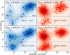 |
Fig. 1. Semi-major axes and masses of planets whose host stars have masses between 0.7 and 2.0 M⊙ and ages between 1.0 and 4.5 Gyr. Top panels: they are separated by the host stars’ phase space density; in the bottom panel, they are separated by the host stars’ peculiar velocity. Typically, a low velocity corresponds to a high phase space density and vice versa. We see an abundance of hot Jupiters in the high-density and the low-velocity populations. We note that stars that cannot be unambiguously assigned to one of the populations are not included, and that some stars have multiple planets. |
3. Phase space density and Galactic velocities
We begin by taking the Sun as a case study. W20 identified the Sun as belonging to a phase-space overdensity. This may reflect the Sun’s origin in a reasonably large, dense cluster (Adams 2010; Pfalzner et al. 2015). However, we note here that the Sun has a rather low peculiar motion for its age (Wielen et al. 1996; Gonzalez 1999). The colour–magnitude diagram for our sample of solar neighbours from Gaia EDR3 is shown in Fig. A.1.
From the solar neighbours within 40 pc, we randomly selected 600 and calculated their local phase space density as described above. We show histograms of the phase space density distribution in Fig. A.2. In common with the distributions for the neighbourhoods of other target stars, the distribution is poorly fit by a single lognormal. Instead, there is typically a steep cut-off at high density, plus a few high-density outliers often associated with known clusters or moving groups, and a shallower tail towards lower densities. A two- (or even higher) component fit is usually superior; in fact, three or more components are often favoured by the Aikake and/or Bayesian Information Criteria, suggesting that the distribution is rather a continuous spectrum than the sum of a high-density and a low-density lognormal. The middle panel of Fig. A.2 shows the decomposition into two components. The Sun lies near the peak of the high-density component. Finally, the right panel shows the probability that the Sun belongs to the high-density component, which we calculate to be 0.88. The probability of belonging to the high-density component actually decreases slightly at high densities on account of the breadth of the low-density component. Visual inspection of several distributions showed that this is usually not too extreme a problem. It was helped by clipping the outliers before fitting the Gaussian mixture model as described above. The Sun is found to have a high probability of belonging to the high-density population, as W20 found. In Fig. A.3, we show the equivalent Gaussian mixture models for the velocity distribution; here, the Sun belongs to the low-velocity component (the probability it belongs to the high-velocity component is 0.03).
As the Mahalanobis density is constructed from both spatial and kinematic information, we now ask which of these is most significant. We begin with the velocities, as suggested in Fig. 1. Figure 2 shows the local phase space density for neighbours of the Sun and BD+20 2184 (alias Pr0201, a hot Jupiter host in the Præsepe open cluster, Quinn et al. 2012), as a function of the stars’ peculiar velocities. In each case, we see a strong correlation: the phase space density is primarily determined by a star’s peculiar velocity. High-density stars are those with low peculiar velocities, low-density stars are those with high peculiar velocities. In Fig. 2, we show the approximate velocity ranges corresponding to membership in the Galactic thin disc, thick disc, and halo via the background colouring (Bensby et al. 2014). The low-density stars appear to be a heterogeneous mix of dynamically hot thin disc stars, thick disc stars, and a handful of halo stars, while the high-density stars are lower velocity thin disc stars. A natural interpretation, then is that stars move from the high-density population to the low-density population as they age and are kinematically heated in the disc.
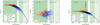 |
Fig. 2. Relationship between a star’s phase space density and its peculiar velocity. Left: local 20th-nearest neighbour phase space density and probability of membership in the high-density population, for 600 stars within 40 pc of the Sun. We show the fitted quartic trend of the density as a function of peculiar velocity. The outlier at ρ ∼ 150 is Gaia EDR3 3277270538903180160 (LP 533-57, HIP 17766), a Hyades member. Centre: residuals to the fit, after the trend is removed. Right: densities and peculiar velocities of 600 neighbours of Pr0201 (BD+20 2184), a hot Jupiter host in the Præsepe cluster. Pr0201 and other Præsepe members stand out from the trend. Green background shading shows the approximate bounds for membership in the Galactic thin disc, thick disc, and halo from Bensby et al. (2014). |
We also see in Fig. 2 the Præsepe cluster at |v|≈30 − 40 km s−1, standing out from the field star trend. The field star population is rather smooth; we detrend this in the next section.
In contrast, large-scale spatial structure (i.e. 10s of pc) has little influence on the phase space density. Figure A.4 shows the local phase space density for neighbours of the Sun and BD+20 2184. For the Sun, we see little large-scale spatial structure; the Mahalanobis phase space density of a star is not strongly dependent on its distance to the Sun. For the neighbours of BD+20 2184, the other Præsepe members are clearly identified by the Mahalanobis density measure as a distinct group, attaining densities of ≳103 within around 10 pc of the target. However, most of the high-density stars as defined by the Gaussian mixture model are not cluster members; 167 high-density stars lie beyond 20 pc of BD+20 2184, and only 74 within 20 pc, those beyond 20 pc having furthermore densities only a little higher than the rest of the field star population, rather than orders of magnitude higher, as is the case for the cluster members.
4. Hunting for a trend in the residuals
We now investigate whether there is any correlation of phase space density with the presence of a hot Jupiter after correcting for the dependence of phase space density on peculiar velocity. Are hot Jupiter hosts high density when compared to stars of similar kinematics? This could be the case if, for example, stars are born from regions of similar |v| but different densities, and this density difference persists as the stars are heated in the disc.
First we detrended the log ρ − log|v| relation. For each of our host stars, we fitted a quartic polynomial to log ρ as a function of log|v| for each of its sample of neighbours. The example of the Sun is shown in Fig. 2. In performing this fit, we excluded densities greater than 50 to avoid the fit being biased by clusters: we wish to fit only field stars. We see in Fig. 2 that, although the Sun is a high-density host, it lies very close to the fitted trend and is quite unremarkable given its cold kinematics.
We repeated this detrending for each of a sample of hot Jupiter hosts (planet mass ≥50 M⊕, planet semi-major axis ≤0.2 au, stellar mass ∈[0.7, 2.0] M⊙2), as well as for a control sample of cold Jupiter hosts (same criteria, except with a semi-major axis > 0.2 au). We show the phase space densities as a function of peculiar velocity in the left-hand panel in Fig. 3; both populations follow a similar trend to the Solar neighbours in Fig. 2. The marginal distributions of both peculiar velocity and phase space density differ significantly (p = 7.6 × 10⁻⁴ and p = 1.1 × 10⁻⁴ on KS tests), with the hot Jupiter hosts having lower velocities and higher densities. Our velocity dispersions for the hot and cold Jupiter hosts are 37.2 km s−1 and 43.3 km s−1 respectively, which are similar to the values obtained by Hamer & Schlaufman (2019)3. In the right-hand panel, we show the residuals of each host star to its fitted trend. The marginal distributions of these residuals are statistically indistinguishable (p = 0.40 on a KS test). Thus, after accounting for the lower velocity dispersion, there is no evidence that the hot Jupiter hosts are located in denser regions of phase space compared to the cold Jupiter control sample.
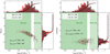 |
Fig. 3. Comparison of velocities and phase space densities for hot Jupiter and cold Jupiter hosts. Left: phase space density versus peculiar velocity for hot Jupiter host stars (HJs) and for cold Jupiter host stars (CJs). Both marginal distributions (top and right sub-panels) are statistically significantly different. The KS-test p values are shown in the figure. HJ hosts have lower velocity and higher density than CJ hosts. Right: residuals to the detrended phase space density versus peculiar velocity for the same stars. The difference in the distribution of residuals between the hot and cold Jupiter populations is not significant (pKS, residuals = 0.40). |
In Appendix A.4, we describe an alternative control experiment, in which we compare the hot Jupiter hosts to the 600 randomly chosen neighbours of the Sun. Again, we find that after accounting for the dependence of the phase space density on velocity, there is no evidence that hot Jupiter hosts are in regions of high density compared to stars with similar kinematics.
5. Discussion
We have now demonstrated that the main determinant of a star’s 6D phase space density is the magnitude of its peculiar motion, that is, how much its Galactic orbit deviates from a circular orbit exactly in the Galactic plane. At the present time, and for the past ∼8 Gyr, stars have been typically born close to the Galactic midplane with a low peculiar velocity, and they are heated with age through interactions with matter inhomogeneities in the Galaxy. This heating occurs on a timescale of Gyr; for eample, with the good asteroseismic ages derivable from Kepler data, Miglio et al. (2021) find that the vertical velocity dispersion for thin disc stars rises from ≈10 km s−1 at an age of 1 Gyr to ≈20 km s−1 at an age of 10 Gyr. The age–velocity relation for the exoplanet host stars with ages given in the NASA Exoplanet Archive is shown in Fig. 4. We caution that these ages come with large errors, as most exoplanet hosts are main-sequence stars and are, moreover, not derived homogeneously (see Adibekyan et al. 2021a for discussion on this). Nonetheless, we do see an increase in the velocity dispersion with age.
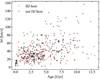 |
Fig. 4. Age–velocity relation for exoplanet host stars with ages given in the NASA Exoplanet Archive. Stars are divided into hot Jupiter hosts and non-hot Jupiter hosts. Error bars on the ages are not shown (indeed, they are not always available) but can easily reach several Gyr. |
This age–velocity relation pertains to the Galactic thin disc. A chemically distinct and kinematically hotter stellar population also exists (the thick disc,), and its stars have a higher velocity dispersion even than thin disc stars of comparable age (Miglio et al. 2021). However, the existence of a clean kinematic separation and the exact relation of kinematics to abundances and to the early history of the Galaxy are still debated (see, e.g. discussion in Agertz et al. 2021). In principle, a clean kinematic separation between thin and thick discs could be a natural way to interpret the stellar phase space densities, with high-density stars being thin disc members and low-density stars being thick disc members. However, when we use the rough kinematic classifications from Bensby et al. (2014), that is, thin disc stars at |v|< 50 km s−1 and thick disc stars at 70 km s−1 ≲ |v|≲180 km s−1, we see that the low-density stars are drawn from both the thick disc and the heated end of the thin disc, with a handful of halo stars as well (see Fig. 2). It is likely that the thick disc stars formed on kinematically hot orbits early in the Galaxy’s history due to early mergers and the turbluent nature of the gas disc at early times (Bird et al. 2013; Agertz et al. 2021; Renaud et al. 2021), and they have maintained their higher velocity dispersion (e.g. Miglio et al. 2021) to the present day. This does not affect our argument, since these stars are all old and kinematically hot, and thus have a low phase space density.
As the high-density stars are kinematically cold and, therefore, young on average, and the low-density stars are a mix of old thick disc stars and old heated thin disc stars, the stellar age naturally suggests itself as an explanation for the overabundance of hot Jupiters orbiting high-density hosts. Hot Jupiters can spiral into their host stars under tidal drag (e.g. Jackson et al. 2009; Levrard et al. 2009; Collier Cameron & Jardine 2018), and if the tidal dissipation is effective enough, the timescale for this is also ≲ Gyrs, similar to that for kinematic heating of the host star. Hamer & Schlaufman (2019) previously identified that hot Jupiter hosts have colder kinematics than cold Jupiter hosts, with similar values of the velocity dispersions to those we have found, and they found that this difference corresponds to tidal decay of hot Jupiter orbits if the tidal quality factor  . Hot Jupiter hosts, then, are predominantly in high-density regions of phase space because of a bias towards detecting the hot Jupiters around young stars before their tidal destruction, a bias noted by Collier Cameron & Jardine (2018). A potential confounding factor we did not consider is stellar metallicity, which has a strong influence on the probability of forming a giant planet (Fischer & Valenti 2005). However, in the solar neighbourhood the age–metallicity relation is rather flat back to ages of around 10 Gyr (Freeman & Bland-Hawthorn 2002; Sahlholdt & Lindegren 2021); for very old stars such as the thick disc, both metallicity and α-element abundance may affect planet formation (Adibekyan et al. 2021b).
We note that we do not show that there is no impact of birth environment on planetary system architecture, only that the differences found through the phase space method primarily arise as a result of age and that nothing is seen when this confounding factor is removed, at least for the hot Jupiters. Surveys directly looking at planets in clusters (e.g. Rizzuto et al. 2020; Nardiello et al. 2020) could address this, but conclusions may be tentative because of the low yield of discoveries. Brucalassi et al. (2016, 2017) found a higher hot Jupiter rate in the M67 open cluster than in the field, but this relies on only three hot Jupiters found in the cluster. There are also other trends found by W20 and subsequent papers (Kruijssen et al. 2020; Chevance et al. 2021; Longmore et al. 2021) that must be explained; we note, however, that the finding of Chevance et al. (2021) that there is a stronger gradient in planetary radius in multi-planet systems orbiting low-density hosts may also be an age effect, as this gradient can result from photoevaporation of the planets’ atmospheres (Owen & Wu 2013), and the older low-density stars have more time for this process to proceed. The trend in multiplicity found by Longmore et al. (2021) is harder to explain: they found that low-density hosts have more multiple systems than high-density hosts. This would seem to go against an age dependence (multiplicity should reduce with time), but we note that their good-quality low-density samples had only five or six stars, and a larger sample would be required to confirm or refute this.
We followed W20 in using the heterogeneous sample of exoplanets provided by the NASA Exoplanet Archive. Recently, Adibekyan et al. (2021a) used a smaller homogeneous sample to look for differences between the high-density and low-density populations; the sample was unfortunately too small to see a significant difference. A difference did emerge in a larger sample, although Adibekyan et al. (2021a) noted that the low-density hosts are older (with a homogeneous age determination) than the low-density hosts. This again underlines the importance of correcting for age. We finish with two further caveats for further studies that may wish to look for trends after the age dependence is removed: first, the differential completeness of Gaia across a target star’s neighbourhood should be accounted for (see Fig. A.5); and second, coherent structures can arise in velocity space among stars of varying ages through interactions with matter inhomogeneities in the Galaxy (e.g. De Simone et al. 2004; Antoja et al. 2018; Kushniruk et al. 2020), so phase space overdensities need not reflect a coeval origin in a dense environment4.
6. Conclusions
We revisited the recent finding that hot Jupiters are preferentially found orbiting stars which are located in high-density regions of Galactic phase space in order to independently verfiy this result and attempt to identify the likely explanation. To do so, we made use of stellar kinematic data from Gaia EDR3. Our main findings are as follows:
-
In classifying stars according to their local 6D phase space densities, we verify that hot Jupiter hosts preferentially belong to the population of high phase space density.
-
Phase space density shows an extremely strong anti-correlation with a star’s peculiar velocity with respect to the Local Standard of Rest in the Galaxy. The high phase space density of hot Jupiter hosts is primarily a manifestation of their cold kinematics.
-
After correcting for the dependency of phase space density on peculiar motion, there is no evidence that hot Jupiter hosts lie in denser regions of phase space than other stars.
-
The observed correlation is likely to arise from the bias towards detecting hot Jupiters around younger (and therefore kinematically colder) host stars, before the hot Jupiters are destroyed by tidal orbital decay. We suggest, therefore, that stellar age, and not formation environment, is the dominant factor linking the presence of a hot Jupiter to the host star’s Galactic kinematics.
A Jupyter notebook and ancillary files to reproduce these results are available on Github5. Details about the contents can be found at the link.
From https://exoplanetarchive.ipac.caltech.edu/index.html, accessed 2021 Mar 11.
This is the same definition of hot Jupiters as that used by W20, except that we have removed the age constraint: when including the age constraint, the sample was too small to see a significant difference in either ρ or |v|.
Taking the semi-major axis cut at a = 0.1 au, we find 35.3 km s−1 and 43.7 km s−1, respectively.
While this paper was under review, Kruijssen et al. (2021) submitted a paper linking the phase space densities to features of Galactic dynamics: the ripples within the Galactic disc generated by matter inhomogeneities such as the bar, arms, and satellite galaxies.
Acknowledgments
AJM acknowledges funding from the Swedish Research Council (grant 2017-04945), the Swedish National Space Agency (grant 120/19C), and the Fund of the Walter Gyllenberg Foundation of the Royal Physiographic Society in Lund. This research has made use of the Aurora cluster hosted at LUNARC at Lund University. AJM wishes to thank Ross Church, Sofia Feltzing, Diederik Kruijssen, Steve Longmore, Paul McMillan, Pete Wheatley, Andrew Winter and the anonymous referee for useful comments and discussions. This work has made use of data from the European Space Agency (ESA) mission Gaia (https://www.cosmos.esa.int/gaia), processed by the Gaia Data Processing and Analysis Consortium (DPAC) (https://www.cosmos.esa.int/web/gaia/dpac/consortium). Funding for the DPAC has been provided by national institutions, in particular the institutions participating in the Gaia Multilateral Agreement. This research made use of Astropy, (http://www.astropy.org) a community-developed core Python package for Astronomy (Astropy Collaboration 2013, 2018). This research made use of NumPy (Harris et al. 2020), SciPy (Virtanen et al. 2020), MatPlotLib (Hunter 2007), and Scikit-learn (Pedregosa et al. 2011). This research has made use of the NASA Exoplanet Archive, which is operated by the California Institute of Technology, under contract with the National Aeronautics and Space Administration under the Exoplanet Exploration Program.
References
- Adams, F. C. 2010, ARA&A, 48, 47 [NASA ADS] [CrossRef] [Google Scholar]
- Adams, F. C., Proszkow, E. M., Fatuzzo, M., & Myers, P. C. 2006, ApJ, 641, 504 [NASA ADS] [CrossRef] [Google Scholar]
- Adibekyan, V., Santos, N. C., Demangeon, O. D. S., et al. 2021a, A&A, 649, A111 [NASA ADS] [CrossRef] [EDP Sciences] [Google Scholar]
- Adibekyan, V., Dorn, C., Sousa, S. G., et al. 2021b, Science, 374, 330 [NASA ADS] [CrossRef] [Google Scholar]
- Agertz, O., Renaud, F., Feltzing, S., et al. 2021, MNRAS, 503, 5826 [NASA ADS] [CrossRef] [Google Scholar]
- Antoja, T., Helmi, A., Romero-Gómez, M., et al. 2018, Nature, 561, 360 [Google Scholar]
- Astropy Collaboration (Robitaille, T. P., et al.) 2013, A&A, 558, A33 [NASA ADS] [CrossRef] [EDP Sciences] [Google Scholar]
- Astropy Collaboration (Price-Whelan, A. M., et al.) 2018, AJ, 156, 123 [Google Scholar]
- Bensby, T., Feltzing, S., & Oey, M. S. 2014, A&A, 562, A71 [NASA ADS] [CrossRef] [EDP Sciences] [Google Scholar]
- Bird, J. C., Kazantzidis, S., Weinberg, D. H., et al. 2013, ApJ, 773, 43 [Google Scholar]
- Brucalassi, A., Pasquini, L., Saglia, R., et al. 2016, A&A, 592, L1 [NASA ADS] [CrossRef] [EDP Sciences] [Google Scholar]
- Brucalassi, A., Koppenhoefer, J., Saglia, R., et al. 2017, A&A, 603, A85 [NASA ADS] [CrossRef] [EDP Sciences] [Google Scholar]
- Carrasco, J. M., Evans, D. W., Montegriffo, P., et al. 2016, A&A, 595, A7 [NASA ADS] [CrossRef] [EDP Sciences] [Google Scholar]
- Casagrande, L., & VandenBerg, D. A. 2018, MNRAS, 479, L102 [NASA ADS] [CrossRef] [Google Scholar]
- Chevance, M., Kruijssen, J. M. D., & Longmore, S. N. 2021, ApJ, 910, L19 [NASA ADS] [CrossRef] [Google Scholar]
- Collier Cameron, A., & Jardine, M. 2018, MNRAS, 476, 2542 [Google Scholar]
- de La Fuente Marcos, C., & de La Fuente Marcos, R. 1997, A&A, 326, L21 [NASA ADS] [Google Scholar]
- De Simone, R., Wu, X., & Tremaine, S. 2004, MNRAS, 350, 627 [NASA ADS] [CrossRef] [Google Scholar]
- Fabrycky, D., & Tremaine, S. 2007, ApJ, 669, 1298 [NASA ADS] [CrossRef] [Google Scholar]
- Fischer, D. A., & Valenti, J. 2005, ApJ, 622, 1102 [NASA ADS] [CrossRef] [Google Scholar]
- Freeman, K., & Bland-Hawthorn, J. 2002, ARA&A, 40, 487 [Google Scholar]
- Gaia Collaboration (Prusti, T., et al.) 2016, A&A, 595, A1 [NASA ADS] [CrossRef] [EDP Sciences] [Google Scholar]
- Gaia Collaboration (Brown, A. G. A.) 2018, A&A, 616, A1 [NASA ADS] [CrossRef] [EDP Sciences] [Google Scholar]
- Gaia Collaboration (Brown, A. G. A., et al.) 2021a, A&A, 649, A1 [NASA ADS] [CrossRef] [EDP Sciences] [Google Scholar]
- Gaia Collaboration (Smart, R. L., et al.) 2021b, A&A, 649, A6 [EDP Sciences] [Google Scholar]
- Gilmore, G., & Reid, N. 1983, MNRAS, 202, 1025 [Google Scholar]
- Gonzalez, G. 1999, MNRAS, 308, 447 [NASA ADS] [CrossRef] [Google Scholar]
- Hamer, J. H., & Schlaufman, K. C. 2019, AJ, 158, 190 [Google Scholar]
- Harris, C. R., Millman, K. J., van der Walt, S. J., et al. 2020, Nature, 585, 357 [NASA ADS] [CrossRef] [Google Scholar]
- Hunter, J. D. 2007, Comput. Sci. Eng., 9, 90 [NASA ADS] [CrossRef] [Google Scholar]
- Jackson, B., Barnes, R., & Greenberg, R. 2009, ApJ, 698, 1357 [Google Scholar]
- Kamdar, H., Conroy, C., Ting, Y.-S., et al. 2019a, ApJ, 884, 173 [NASA ADS] [CrossRef] [Google Scholar]
- Kamdar, H., Conroy, C., Ting, Y.-S., et al. 2019b, ApJ, 884, L42 [NASA ADS] [CrossRef] [Google Scholar]
- Kruijssen, J. M. D., Longmore, S. N., & Chevance, M. 2020, ApJ, 905, L18 [Google Scholar]
- Kruijssen, J. M. D., Longmore, S. N., Chevance, M., et al. 2021, ApJ, submitted [arXiv:2109.06182] [Google Scholar]
- Kushniruk, I., Bensby, T., Feltzing, S., et al. 2020, A&A, 638, A154 [NASA ADS] [CrossRef] [EDP Sciences] [Google Scholar]
- Laughlin, G., & Adams, F. C. 1998, ApJ, 508, L171 [NASA ADS] [CrossRef] [Google Scholar]
- Levrard, B., Winisdoerffer, C., & Chabrier, G. 2009, ApJ, 692, L9 [NASA ADS] [CrossRef] [Google Scholar]
- Li, D., Mustill, A. J., & Davies, M. B. 2019, MNRAS, 488, 1366 [NASA ADS] [CrossRef] [Google Scholar]
- Li, D., Mustill, A. J., & Davies, M. B. 2020a, MNRAS, 499, 1212 [Google Scholar]
- Li, D., Mustill, A. J., & Davies, M. B. 2020b, MNRAS, 496, 1149 [Google Scholar]
- Lin, D. N. C., Bodenheimer, P., & Richardson, D. C. 1996, Nature, 380, 606 [Google Scholar]
- Longmore, S. N., Chevance, M., & Kruijssen, J. M. D. 2021, ApJ, 911, L16 [NASA ADS] [CrossRef] [Google Scholar]
- Mahalanobis, P. C. 1936, Proc. National Inst. Sci. India, 2, 49 [Google Scholar]
- Malmberg, D., de Angeli, F., Davies, M. B., et al. 2007a, MNRAS, 378, 1207 [NASA ADS] [CrossRef] [Google Scholar]
- Malmberg, D., Davies, M. B., & Chambers, J. E. 2007b, MNRAS, 377, L1 [NASA ADS] [CrossRef] [Google Scholar]
- Malmberg, D., Davies, M. B., & Heggie, D. C. 2011, MNRAS, 411, 859 [Google Scholar]
- Miglio, A., Chiappini, C., Mackereth, J. T., et al. 2021, A&A, 645, A85 [NASA ADS] [CrossRef] [EDP Sciences] [Google Scholar]
- Nardiello, D., Piotto, G., Deleuil, M., et al. 2020, MNRAS, 495, 4924 [Google Scholar]
- Nordström, B., Mayor, M., Andersen, J., et al. 2004, A&A, 418, 989 [Google Scholar]
- Owen, J. E., & Wu, Y. 2013, ApJ, 775, 105 [Google Scholar]
- Parker, R. J., & Goodwin, S. P. 2009, MNRAS, 397, 1041 [CrossRef] [Google Scholar]
- Parker, R. J., & Quanz, S. P. 2012, MNRAS, 419, 2448 [Google Scholar]
- Pedregosa, F., Varoquaux, G., Gramfort, A., et al. 2011, J. Mach. Learn. Res., 12, 2825 [Google Scholar]
- Pfalzner, S., Davies, M. B., Gounelle, M., et al. 2015, Phys. Scr., 90, 068001 [NASA ADS] [CrossRef] [Google Scholar]
- Quinn, S. N., White, R. J., Latham, D. W., et al. 2012, ApJ, 756, L33 [NASA ADS] [CrossRef] [Google Scholar]
- Rasio, F. A., & Ford, E. B. 1996, Science, 274, 954 [Google Scholar]
- Renaud, F., Agertz, O., Andersson, E. P., et al. 2021, MNRAS, 503, 5868 [NASA ADS] [CrossRef] [Google Scholar]
- Rizzuto, A. C., Newton, E. R., Mann, A. W., et al. 2020, AJ, 160, 33 [Google Scholar]
- Rodet, L., Su, Y., & Lai, D. 2021, ApJ, 913, 104 [NASA ADS] [CrossRef] [Google Scholar]
- Sahlholdt, C. L., & Lindegren, L. 2021, MNRAS, 502, 845 [CrossRef] [Google Scholar]
- Schönrich, R., Binney, J., & Dehnen, W. 2010, MNRAS, 403, 1829 [NASA ADS] [CrossRef] [Google Scholar]
- Spitzer, L., Jr., & Schwarzschild, M. 1951, ApJ, 114, 385 [NASA ADS] [CrossRef] [Google Scholar]
- Virtanen, P., Gommers, R., Oliphant, T. E., et al. 2020, Nat. Methods, 17, 261 [Google Scholar]
- Weidenschilling, S. J., & Marzari, F. 1996, Nature, 384, 619 [Google Scholar]
- Wielen, R. 1977, A&A, 60, 263 [NASA ADS] [Google Scholar]
- Wielen, R., Fuchs, B., & Dettbarn, C. 1996, A&A, 314, 438 [NASA ADS] [Google Scholar]
- Winter, A. J., Clarke, C. J., Rosotti, G., et al. 2018, MNRAS, 478, 2700 [Google Scholar]
- Winter, A. J., Kruijssen, J. M. D., Longmore, S. N., & Chevance, M. 2020, Nature, 586, 528 [Google Scholar]
- Wu, Y., & Murray, N. 2003, ApJ, 589, 605 [Google Scholar]
Appendix A: Additional figures
A.1. Colour–magnitude diagram for solar neighbours
We show the colour–magnitude diagram for our sample of solar neighbours in Figure A.1. We have, in keeping with W20, imposed no quality cuts on the Gaia data (other than the need for parallax to be positive); however, we note that moving from DR2 to EDR3 cleans the CMD considerably, especially of spurious objects below the main sequence. The blob at MG ∼ 8, below the main sequence, is discussed in Gaia Collaboration (2021b), who attributed it to a change at G = 13 in the window of pixels on the CCD surrounding the target (Carrasco et al. 2016). In this paper, we work with the EDR3 data.
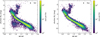 |
Fig. A.1. Colour–magnitude diagrams for all stars within 80 pc of the Sun with Gaia RVs. Left: DR2. Right: EDR3. The Gaia colour and magnitude for the Sun are taken from Casagrande & VandenBerg (2018). |
A.2. Gaussian mixture model
In Figure A.2, we show the Gaussian mixture model for the Sun and 600 of its neighbours, together with the stars’ probability of belonging to the high-density population. We note that this probability begins to decrease slightly for stars with moderately high densities, on account of the breadth of the low-density distribution. Stars at ρ > 50 are assigned Phigh = 1 to alleviate this. We show the equivalent decomposition in velocities in Figure A.3.
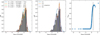 |
Fig. A.2. Gaussian mixture models for the local phase space density of the Sun. Left: One- to ten-component models, together with Aikake and Bayesian information criteria values relative to the best fit. Middle: One- and two-component models, together with the decomposition of the latter. Right: Probability of each star belonging to the high-density component of the two-component model. |
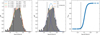 |
Fig. A.3. Gaussian Mixture models for the local peculiar velocity distribution of neighbours of the Sun. Left: One- to ten-component models, together with Aikake and Bayesian information criteria values relative to the best fit. Middle: One- and two-component models, together with the decomposition of the latter. Right: Probability of each star belonging to the high-velocity component of the two-component model. |
A.3. Spatial structure
In Figure A.4, we show the phase space density as a function of distance to the target star, for 600 neighbours of the Sun and of the Præsepe member BD+20 2184. There is little structure seen among the neighbours of the Sun, although there may be a weak trend from 25 to 40 pc; this disappears if we restrict attention to stars with an absolute magnitude MG ≤ 8, and it may reflect the decreasing completeness of Gaia with distance. For BD+20 2184, fellow cluster members stand out at high density close to the target.
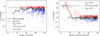 |
Fig. A.4. Local 20th-nearest neighbour phase space density and probability of membership to the high-density population for 600 stars within 40 pc of the Sun (left) and Pr0201 (BD+20 2184, right). We show these as a function of the distance to the target star. |
In Figure A.5, we show the differential completeness of the Gaia EDR3 RV catalogue across a sphere of 80 pc centred on BD+20 2184. Looking at the top panels, we see that the 3D spatial density of stars in the RV catalogue falls by a factor of three between the near side of the sphere and the far side of the sphere. This seems not to induce a strong bias in the spatial density as a function of distance from BD+20 2184 itself, shown in the bottom right panel. The Præsepe cluster clearly stands out as a significant spatial overdensity, beyond which the density is constant. Nevertheless, the potential for the differential completeness to induce a bias should be borne in mind as a potential confounding factor once the main velocity dependence of the phase space density is accounted for.
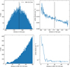 |
Fig. A.5. Differential completeness of the Gaia EDR3 RV catalogue across a sphere of 80 pc centred on BD+20 2184. Left-hand panels show histograms of the number of stars per distance bin, measured from the Sun (top) and from BD+20 2184 (bottom). Right-hand panels show the corresponding 3D spatial density. |
A.4. Alternative detrending comparison
In the main body of the paper (§4), we showed that the phase space density residuals, after the velocity trend is removed, are identical for the hot and cold Jupiter hosts. This implicitly puts all of the phase space densities on the same scale, despite their being constructed from different samples. While the densities are all normalised such that the median of each distribution is unity, and the fitted trends are all quite similar, there is nevertheless a small scatter in the fitted trends. Here, we describe an alternative test that relies only on the ranks of stars within their populations of neighbours, both in terms of phase space density and the residuals after detrending.
As each sample may contain a different number of stars, we first defined fractional ranks between 0 and 1, such that
 (A.1)
(A.1)
and
 (A.2)
(A.2)
where rρ and rres are the ranks (1 being high) of each star in density and in the residuals, and Nsample is the number of stars in the sample. We then compared the hot Jupiter hosts to the neighbours of the Sun. For each hot Jupiter host, we calculated its fractional ranks and paired it up with the nearest-ranked neighbour of the Sun, with rank (in density)
 (A.3)
(A.3)
where Ncontrol = 600 is the number of neighbours of the Sun and fρ,HJ is the fractional density rank of the hot Jupiter host. We then constructed a control distribution of residuals by selecting the fractional residuals ranks of the solar neighbours whose density ranks are given by rcomp.
This procedure is illustrated in Figure A.6. The fractional ranks for the hot Jupiter hosts are shown in the left-hand panel. The density of points increases towards the bottom left. The increase towards the left reflects the tendency for hot Jupiter hosts to have high phase space densities. The increase towards the bottom shows that they tend to have high residuals after detrending. However, even an unbiased sample can show a tendency for high density to correspond with high residuals. This is demonstrated in the middle panel of Figure A.6, where we show the equivalent rankings for the 600 neighbours of the Sun. In the right-hand panel of Figure A.6, we show the comparison between the hot Jupiter sample and the control sample drawn from the centre panel. The hot Jupiter sample and the control sample are then indistinguishable on a KS test (p = 0.32). We note that a set of randomly-selected neighbours of the Sun would give a uniform distribution.
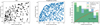 |
Fig. A.6. Comparison between hot Jupiter hosts and a control sample of stars near the Sun. Left: The fractional rank (rank among neighbours divided by number of neighbours) in phase space density, and in residuals to the detrended phase space density, for all 198 hot Jupiter hosts. Darker symbols are stars with more neighbours in Gaia EDR3. Centre: Same, but for 600 neighbours of the Sun. Right: Histogram of the fractional residuals rank for the hot Jupiter hosts (blue for differential, orange for cumulative) and for the fractional residuals rank of 198 neighbours of the Sun chosen to have the same density fractional rank as the hot Jupiter hosts (green for differential, red for cumulative). The KS test p-value comparing the two distributions is also displayed, showing that they are statistically indistinguishable. |
All Figures
|
Fig. 1. Semi-major axes and masses of planets whose host stars have masses between 0.7 and 2.0 M⊙ and ages between 1.0 and 4.5 Gyr. Top panels: they are separated by the host stars’ phase space density; in the bottom panel, they are separated by the host stars’ peculiar velocity. Typically, a low velocity corresponds to a high phase space density and vice versa. We see an abundance of hot Jupiters in the high-density and the low-velocity populations. We note that stars that cannot be unambiguously assigned to one of the populations are not included, and that some stars have multiple planets. |
| In the text | |
|
Fig. 2. Relationship between a star’s phase space density and its peculiar velocity. Left: local 20th-nearest neighbour phase space density and probability of membership in the high-density population, for 600 stars within 40 pc of the Sun. We show the fitted quartic trend of the density as a function of peculiar velocity. The outlier at ρ ∼ 150 is Gaia EDR3 3277270538903180160 (LP 533-57, HIP 17766), a Hyades member. Centre: residuals to the fit, after the trend is removed. Right: densities and peculiar velocities of 600 neighbours of Pr0201 (BD+20 2184), a hot Jupiter host in the Præsepe cluster. Pr0201 and other Præsepe members stand out from the trend. Green background shading shows the approximate bounds for membership in the Galactic thin disc, thick disc, and halo from Bensby et al. (2014). |
| In the text | |
|
Fig. 3. Comparison of velocities and phase space densities for hot Jupiter and cold Jupiter hosts. Left: phase space density versus peculiar velocity for hot Jupiter host stars (HJs) and for cold Jupiter host stars (CJs). Both marginal distributions (top and right sub-panels) are statistically significantly different. The KS-test p values are shown in the figure. HJ hosts have lower velocity and higher density than CJ hosts. Right: residuals to the detrended phase space density versus peculiar velocity for the same stars. The difference in the distribution of residuals between the hot and cold Jupiter populations is not significant (pKS, residuals = 0.40). |
| In the text | |
|
Fig. 4. Age–velocity relation for exoplanet host stars with ages given in the NASA Exoplanet Archive. Stars are divided into hot Jupiter hosts and non-hot Jupiter hosts. Error bars on the ages are not shown (indeed, they are not always available) but can easily reach several Gyr. |
| In the text | |
|
Fig. A.1. Colour–magnitude diagrams for all stars within 80 pc of the Sun with Gaia RVs. Left: DR2. Right: EDR3. The Gaia colour and magnitude for the Sun are taken from Casagrande & VandenBerg (2018). |
| In the text | |
|
Fig. A.2. Gaussian mixture models for the local phase space density of the Sun. Left: One- to ten-component models, together with Aikake and Bayesian information criteria values relative to the best fit. Middle: One- and two-component models, together with the decomposition of the latter. Right: Probability of each star belonging to the high-density component of the two-component model. |
| In the text | |
|
Fig. A.3. Gaussian Mixture models for the local peculiar velocity distribution of neighbours of the Sun. Left: One- to ten-component models, together with Aikake and Bayesian information criteria values relative to the best fit. Middle: One- and two-component models, together with the decomposition of the latter. Right: Probability of each star belonging to the high-velocity component of the two-component model. |
| In the text | |
|
Fig. A.4. Local 20th-nearest neighbour phase space density and probability of membership to the high-density population for 600 stars within 40 pc of the Sun (left) and Pr0201 (BD+20 2184, right). We show these as a function of the distance to the target star. |
| In the text | |
|
Fig. A.5. Differential completeness of the Gaia EDR3 RV catalogue across a sphere of 80 pc centred on BD+20 2184. Left-hand panels show histograms of the number of stars per distance bin, measured from the Sun (top) and from BD+20 2184 (bottom). Right-hand panels show the corresponding 3D spatial density. |
| In the text | |
|
Fig. A.6. Comparison between hot Jupiter hosts and a control sample of stars near the Sun. Left: The fractional rank (rank among neighbours divided by number of neighbours) in phase space density, and in residuals to the detrended phase space density, for all 198 hot Jupiter hosts. Darker symbols are stars with more neighbours in Gaia EDR3. Centre: Same, but for 600 neighbours of the Sun. Right: Histogram of the fractional residuals rank for the hot Jupiter hosts (blue for differential, orange for cumulative) and for the fractional residuals rank of 198 neighbours of the Sun chosen to have the same density fractional rank as the hot Jupiter hosts (green for differential, red for cumulative). The KS test p-value comparing the two distributions is also displayed, showing that they are statistically indistinguishable. |
| In the text | |
Current usage metrics show cumulative count of Article Views (full-text article views including HTML views, PDF and ePub downloads, according to the available data) and Abstracts Views on Vision4Press platform.
Data correspond to usage on the plateform after 2015. The current usage metrics is available 48-96 hours after online publication and is updated daily on week days.
Initial download of the metrics may take a while.