| Issue |
A&A
Volume 657, January 2022
|
|
|---|---|---|
| Article Number | L3 | |
| Number of page(s) | 11 | |
| Section | Letters to the Editor | |
| DOI | https://doi.org/10.1051/0004-6361/202142276 | |
| Published online | 07 January 2022 | |
Letter to the Editor
Gyrochronological dating of the stellar moving group Group X
1
INAF-Catania Astrophysical Observatory, Via S. Sofia, 78, 95123 Catania, Italy
e-mail: This email address is being protected from spambots. You need JavaScript enabled to view it.
2
Aix Marseille Univ., CNRS, CNES, LAM, Marseille, France
3
Istituto Nazionale di Astrofisica – Osservatorio Astronomico di Padova, Vicolo dell’Osservatorio 5, 35122 Padova, Italy
4
Dipartimento di Fisica e Astronomia Galileo Galilei, Vicolo dell’Osservatorio 3, 35122 Padova, Italy
5
INAF – Astronomical Observatory of Palermo, Piazza del Parlamento 1, 90134 Palermo, Italy
6
INAF – Osservatorio Astronomico di Roma, Via Frascati 33, 00040 Monte Porzio Catone, RM, Italy
Received:
22
September
2021
Accepted:
6
December
2021
Abstract
Context. Gyrochronology is one of the methods currently used to estimate the age of stellar open clusters. Hundreds of new clusters, associations, and moving groups unveiled by Gaia and complemented by accurate rotation period measurements provided by recent space missions such as Kepler and TESS are allowing us to significantly improve the reliability of this method.
Aims. We use gyrochronology, that is, the calibrated age-mass-rotation relation valid for low-mass stars, to measure the age of the recently discovered moving group Group X.
Methods. We extracted the light curves of all candidate members from the TESS full frame images and measured their rotation periods using different period search methods.
Results. We measured the rotation period of 168 of a total of 218 stars and compared their period-colour distribution with those of two age-benchmark clusters, the Pleiades (125 Myr) and Praesepe (625 Myr), as well as with the recently characterised open cluster NGC 3532 (300 Myr).
Conclusions. As result of our analysis, we derived a gyro age of 300 ± 60 Myr. We also applied as independent methods the fitting of the entire isochrone and of the three brightest candidate members individually with the most precise stellar parameters, deriving comparable values of 250 Myr and 290 Myr, respectively. Our dating of Group X allows us to definitively rule out the previously proposed connection with the nearby but much older Coma Berenices cluster.
Key words: stars: low-mass / stars: rotation / stars: activity / stars: pre-main sequence / stars: evolution / open clusters and associations: general
© ESO 2022
1. Introduction
Stellar age is a key parameter in several astrophysical contexts, from exo-planetary science, where the derived values of the planet’s physical parameters depend on the age of the host star (see e.g. Carleo et al. 2021), to Milky Way studies, where Galactic formation and evolution models can be constrained if the age of numerous field and cluster stars is known (see e.g. Hayden et al. 2020). An accurate estimate of the ages of coeval stars in stellar clusters and associations is more reliable if compared to the results obtained for Galactic field stars. Some techniques for the estimation of the ages of cluster members are based on the comparison between measurable stellar parameters and stellar evolutionary models (e.g. main-sequence and turn-off isochrone fitting; Pont & Eyer 2004), and lithium-depletion boundary fitting (Stauffer et al. 1998; Messina et al. 2016). Other methods make use of calibrated empirical relationships (e.g. the gyrochronology; Angus et al. 2019; Barnes 2007), specific element abundance ratios (e.g. Maldonado et al. 2015), and activity proxies (e.g. Zhang et al. 2019; Messina 2021). Asteroseismic analysis allows us to obtain the age of single stars in our Galaxy (Lebreton & Montalbán 2009). Firm calibrations are required in the case of methods based on empirical calibrations, and, usually, different approaches are suitable for limited regions of the parameter space, making age determination a particularly challenging task (see Soderblom 2010 for a review). However, a combination of different techniques for the estimate of the ages allows us to obtain a final robust result (see e.g. Desidera et al. 2015).
The recent Gaia Early Third Data Release (Bailer-Jones et al. 2021) is unveiling a plethora of stellar open clusters and associations (e.g. Cantat-Gaudin et al. 2018). Complementary measurements of rotation periods of the candidate members of newly discovered clusters and associations from all-sky ground-based projects (e.g. SuperWASP; Pollacco et al. 2006) and space-borne missions (e.g. Kepler/K2, Borucki 2018), not only allow the membership to be solidified through gyrochronology but also provide the opportunity to get a robust calibration of the gyrochronology over a large range of ages.
Usually, as first step, the rotation period-colour distribution of newly discovered clusters is compared with known age-benchmark clusters, such as the Pleiades and Praesepe. Then, the isochrone fitting and any other available age diagnostics are also used to secure consistent results. In a following step, the inferred ages of the new clusters are used to improve the age sampling of the gyrochronology. This approach allowed Curtis et al. (2019) to discover the Pisces-Eridanus stellar stream and to estimate a gyrochronological age of about 120 Myr and allowed Bouma et al. (2021) to discover a halo for the open cluster NGC 2516 and estimate a gyrochronological age of about 150 Myr, to mention just a couple recent studies. In this framework, we present the results of our analysis of the newly discovered moving group Group X.
Group X is a nearby moving group (d ∼ 101 pc; Tang et al. 2018). Based on the Gaia Data Release 1 TGAS (Tycho-Gaia Astrometric Solution) data, Oh et al. (2017) first discovered an initial sample of 27 candidate members, which were subsequently confirmed as a group by Faherty et al. (2018). The most recent analysis was carried out by Tang et al. (2019), who discovered up to 218 candidate members, including the 27 candidates listed by Oh et al. (2017). Moreover, they ruled out the previously proposed connection with the nearby Coma Berenices group, providing clear evidence that they are two dynamically distinct systems. Group X is an interesting example of a moving group at the final stage of disruption by the Galactic tides, as evidenced by the irregular and elongated space distribution of its members. The isochrone fitting method applied by Tang et al. (2019) yielded an age estimate of 400 Myr.
In this work we used astrometric and kinematic data made available by Gaia, rotation periods from TESS (Transiting Exoplanet Survey Satellite), colour-magnitude diagrams (CMDs) suitable for isochrone fitting, and other age diagnostics (such as the lithium line and activity indicators), which we are collecting for a selection of members to estimate the age and to add a new age tick mark in the rotation-mass-age relation of low-mass stars.
In Sect. 2 we describe the photometric data on which our analysis is based. In Sect. 3 we present the CMD and the results of our period search analysis. Discussion and conclusions are presented in Sects. 4 and 5.
2. Data
We used the data collected by TESS in the second year of its main mission (Sectors 14–26) between July 18, 2019, and July 4, 2020. We obtained the light curves of the stars from the full frame images (FFIs) by using the PATHOS pipeline described in Nardiello et al. (2019). Briefly, we used the software img2lc (written in FORTRAN 90/95 + OPENMP) developed by Nardiello et al. (2015, 2016) for ground-based instruments to extract the light curves from the FFIs. This software takes as input the FFIs, empirical point spread function (PSF) arrays, and an input catalogue, and, after modelling and subtracting the neighbour stars to each target source in the input catalogue, it measures the flux of the target star with four different apertures (1-px, 2-px, 3-px, 4-px aperture) and PSF-fitting photometry. Different apertures work better for stars of different magnitudes, and we selected the best aperture for each target, comparing their mean rms distributions as described in detail by Nardiello (2020). The light curves are then corrected by using the cotrending basis vectors as described in Nardiello et al. (2020, 2021). As input catalogue we used the list of stars published by Tang et al. (2019), which contains 218 likely members of Group X. We extracted 770 light curves: only 3 stars are observed in a single sector, 18 stars are observed in 2 sectors, 88 stars are observed in 3 sectors, 89 stars are observed in 4 sectors, 14 stars in 5 sectors, 5 stars in 6 sectors, and 1 star is observed in 11 sectors.
Light curves will be released on the Mikulski Archive for Space Telescopes (MAST) as a High Level Science Product (HLSP) under the project PATHOS1. A detailed description of the light curves is given in Nardiello et al. (2019).
3. Analysis
3.1. Colour-magnitude diagram
The CMD presented in Fig. 1 was obtained using the Gaia Data Release 2 (DR2) parallaxes and G magnitudes complemented with 2MASS (Two Micron All-Sky Survey) Ks magnitudes (Cutri et al. 2003). Black and red bullets are used to distinguish between non-periodic and periodic candidate members, respectively (see the following subsection). Seven periodic candidate members with a nearby companion (separation ρ < 3″) are unresolved in the 2MASS photometry. For these candidates, we computed the correction to be applied to the G − Ks colour, using the G magnitudes and parallaxes of the components and the PARSEC models of Bressan et al. (2012) computed for an age of 400 Myr and deriving the expected Ks magnitudes for both components (see e.g. Sect. 3 in Messina 2019). Finally, colours were corrected for interstellar reddening. We first calculated the E(B − V) of each star by using the PYTHON routine mwdust2 (Bovy et al. 2016) and the Combined19 dust map (Drimmel et al. 2003; Marshall et al. 2006; Green et al. 2019), and then we transformed it into E(G − K) according to the method presented in Bessell & Brett (1988). We found that the correction for the interstellar reddening results in a slightly smaller scatter from the isochrone (see ahead) if the average value, ⟨E(G − Ks)⟩ = 0.015 ± 0.006 mag (E(B − V) = 0.005 mag), is applied instead of correcting each target for its own reddening. For instance, this reddening is very close to the null reddening computed for the nearby Coma Berenices cluster (Tang et al. 2018). In the following analysis, the average reddening is applied.
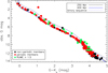 |
Fig. 1. CMD for the Group X candidate members (Tang et al. 2019), with the 250 Myr (solid black line) and 400 Myr (solid blue line) isochrones overplotted. Dashed lines represent the sequence of equal-mass main-sequence binaries. Errors on magnitudes and colours are smaller than the symbol size. |
The CMD was compared with a series of isochrones based on PARSEC models of Bressan et al. (2012), which span a range of ages from 150 Myr to 700 Myr. The isochrone that best describes the observed CMD has an age of 250 Myr. A slightly better description, but of only the upper bluer part of the CMD, is provided by the isochrone of 400 Myr.
We also plot, as dotted lines, the sequences of equal-mass binaries for both ages. We note a number of candidates (27) that lie either significantly above the equal-mass binary isochrone (#89, #102, and #103) or in the magnitude interval between the single and the equal-mass binary sequence. To further investigate their nature and to unveil the presence of unresolved close binaries among them, we used the re-normalised unit weight error (RUWE; see Lindegren et al. 2018). All candidates with RUWE > 1.5 (a total of 22) are overplotted in green. The following candidates, although significantly displaced from the single star sequence, were not classified according to the RUWE as close binaries: #27, #38, #40, #47, #58, #102, #143, #158, #170, #173, #183, #184, #201, and #208.
These outliers may be still members but may be suffering from an underestimated correction for reddening. Justifying the position in the CMD of star #102 is more problematic. On the other side, the inability of the isochrone to adequately fit the bottom end of the sequence is a known problem (see e.g. Bell et al. 2012; Morrell & Naylor 2019), and its discussion is beyond the scope of the present study.
As a complementary approach to estimating the age of Group X, we also considered the three brightest candidate members individually with the most precise determination of their stellar parameters (#51: 84 UMa, #28: HD 118214, and #45: HD 119765), exploiting the PARAM online tool for the Bayesian estimation of stellar parameters (da Silva et al. 2006) to obtain the most probable age. The individual ages are 240 ± 100, 320 ± 110, and 300 ± 110 Myr, respectively. This supports an age with a mean value of 290 Myr as the most probable one.
3.2. Rotation period search
We analysed the TESS light curves of the Group X candidate members to measure the rotation period using three different methods: generalised Lomb-Scargle (GLS; Zechmeister & Kürster 2009), (CLEAN; Roberts et al. 1987), and the autocorrelation function (ACF; McQuillan et al. 2013). Details and examples of the use of these methods can be found in Messina et al. (2017) for GLS and CLEAN, and McQuillan et al. (2013) for ACF. We used more than one method in order to provide a ‘grade’ of confidence on the correctness of the measured rotation periods. If the values of the rotation periods were found by all three methods to be similar within the respective uncertainties, we assigned a quality grade ‘A’; when only two methods found the same value, we assigned a grade ‘B’. Period estimates differing in all three methods were not considered. Since most stars were observed in more TESS sectors, our period search was performed in each available sector. Generally, the same rotation period was found in subsequent sectors, increasing the robustness of our measurement results. An example case of periodogram analysis is given in Fig. 2.
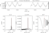 |
Fig. 2. Example case of periodogram analysis of target #57. Top panel: TESS magnitude time series. Bottom: GLS periodogram (left), CLEAN periodogram (middle), and ACF (right), with the solid vertical red lines indicating the rotation period. |
We selected only rotation periods with false alarm probability (FAP) < 0.1%. The FAP was computed using the analytical formulae of Horne & Baliunas (1986), which are valid for evenly spaced time series data. We followed the method used by Lamm et al. (2004) to compute the errors associated with the period determinations (see e.g. Messina et al. 2010, for details). From a total sample of 218 stars, we measured 150 periods with grade A and 18 periods with grade B. In Fig. 3 we plot the rotation period distribution of Group X. We use different symbols to indicate grade A (filled circles) and grade B (diamonds) periods and squared symbols to indicate the mentioned outliers in the CMD (red for RUWE > 1.5 and blue for RUWE < 1.5). In Table A.1 we list the rotation periods with respective uncertainty, grade, and the TESS sector in which the same value of period was measured.
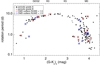 |
Fig. 3. Distribution of stellar rotation periods versus de-reddened colour for the periodic candidate members of Group X. |
As mentioned, the PATHOS pipeline subtracts from the target the flux of any neighbour star in the adjacent pixels (i.e. at distances ρ > 10″). As a consequence of this and the dilution effect, any effect of variability in the residual flux of the nearby stars becomes negligible. On the contrary, the flux of neighbour stars at distances ρ < 10″ is not removed by the pipeline and it may contribute significantly to the observed variability.
A total of 17 periodic stars in our sample (marked with an asterisk in Table A.1) have one visual companion detected in the Gaia DR2 but are unresolved in the TESS photometry at a separation of ρ ≲ 10″ and with a magnitude difference of ΔG < 3 mag (all have RUWE < 1.5). We inspected the periodograms of these 17 candidate members and found nine cases (stars #12, #17, #27, #137, and #141 and the systems #29&30 and #148&149) with a significant secondary period. The secondary period can be interpreted as the rotation period of the nearby companion (see e.g. Messina 2019; Bonavita et al. 2021; Tokovinin & Briceño 2018). On the other hand, stars #39 and #63, which have no detected nearby companion in the Gaia DR2, have clear evidence of a secondary period, P = 0.3639 d and P = 0.4646 d, respectively.
4. Discussion
As mentioned in Sect. 1, the main scope of the present work is to estimate the age of Group X via gyrochronology, providing independent support to the membership by Tang et al. (2019). This is accomplished by comparing the distribution of the rotation period with those of primary age-benchmark open clusters, specifically the Pleiades with an age of ∼125 Myr (Stauffer et al. 1998) and Praesepe with an age of ∼625 Myr (Brandt & Huang 2015). A comparison with the NGC 3532 (∼300 Myr; Fritzewski et al. 2021) and M 48 (∼450 Myr; Barnes et al. 2015) clusters is also done. Rotation periods of Pleiades members are taken from Rebull et al. (2016), those of Praesepe from Rebull et al. (2017), those of NGC 3532 from Fritzewski et al. (2021), and those of M 48 from Barnes et al. (2015).
Colours were de-reddened by adopting a colour excess E(B − V) = 0.045 mag for the Pleiades and E(B − V) = 0.027 mag for Praesepe (Gaia Collaboration 2018) and E(B − V) = 0.035 mag for NGC 3532 (Fritzewski et al. 2021) and E(B − V) = 0.08 mag for M 48 (Barnes et al. 2015). Finally, (G − Ks)0 colours were transformed into B − V colours using the calibration by Pecaut & Mamajek (2013).
To compare the period distribution of Group X with those of the Pleiades and Praesepe and to derive a quantitative estimate of the age of Group X, we selected the sequence of slow rotators, that is, the colour range 0.5 < (B − V)0 < 1.3 mag, where the dependence on the age of the rotation period is better defined (an almost one-to-one correspondence between colour and period). As shown in Fig. 3, both single stars and candidate binaries that lie between the single and binary sequences follow the same period distribution. Therefore, we opted to include all of them in the process of age estimate. We adopted a colour binning of 0.10 mag, then for each bin we computed the median rotation period, and, finally, we fitted a polynomial to the sequence of median values (the solid blue and red lines in the bottom panel of Fig. 4). We assumed that in the age interval between the Pleiades and Praesepe the period slowdown has a functional form of the type
 (1)
(1)
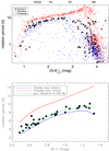 |
Fig. 4. Comparison of colour-period distribution of Group X with age-benchmark open clusters. Top panel: distribution of stellar rotation periods of Group X with the Pleiades and Praesepe distributions overplotted. Bottom panel: distribution of the rotation periods of slow rotators of Group X versus B − V colour, with the polynomial fits to median rotation periods of slow rotators in the Praesepe (red line) and Pleiades (blue line) clusters and, as an example, the gyro-sequence corresponding to an age of 300 Myr (green line), according to the Mamajek & Hillenbrand (2008) coefficients, overplotted. |
We inferred the age of each candidate member, finding, as shown in Fig. 5, a bimodal-like distribution with the bulk of members at an age of 350 Myr (∼360 Myr using Mamajek & Hillenbrand 2008 coefficients) and a minority, ∼25%, at an age of about 230 Myr. For the whole moving group, we obtain an average value of 309 ± 60 Myr using the a, b, c, and n coefficients from Mamajek & Hillenbrand (2008) and 297 ± 50 Myr using the Angus et al. (2015) coefficients. Their average value of 303 ± 60 Myr is in agreement within the uncertainties with the isochronal age derived by us (i.e. 250 Myr) and in agreement with the age of the three brightest stars derived with PARAM (i.e. 290 Myr). We note that in the selected colour range for the gyrochronological estimate of age (0.5 < (B − V)0 < 1.3 mag), all visual binaries have their components at distances ρ > 150 au, which is sufficiently distant to neglect any effects of tides on the rotation period evolution (see e.g. Messina 2019).
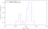 |
Fig. 5. Distribution of ages of individual candidate members as derived by the relations of Angus et al. (2015, solid blue line) and by Mamajek & Hillenbrand (2008, dotted red line). |
Finally, the age of ∼300 Myr for Group X is also supported by the comparison with the rotation period distribution of the NGC 3532 open cluster, which has an estimated age of 300 Myr. As shown in Fig. 6, the two distributions are almost undistinguishable for (G − Ks)0 < 2.3 mag. However, in the colour range 2.3 < (G − Ks)0 < 3.3 mag, the Group X candidate members, which are all found to be periodic, all rotate faster than their counterpart slow-rotator members of NGC 3532. In the mentioned colour range, all candidate members being periodic, it is unlikely that the absence of longer rotation periods arises from the insensitivity of TESS data to rotation periods longer than 10−12 days.
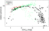 |
Fig. 6. Comparison of the rotation period distributions of Group X with the coeval NGC 3532 and with the older M 48 open clusters. |
It is worth noting that the possibility of measuring the age of stellar clusters by means of gyrochronology makes the search for exo-planets around their members especially relevant. This is the case of one TESS target of interest identified among the candidate members of Group X and whose characterisation (Nardiello et al., in prep.) greatly benefits from the age determined in the present study.
5. Conclusions
We have explored the rotational properties of the late-type candidate members of the recently discovered moving group Group X, which has a total of 218 candidate members. All the candidate members were observed by TESS in one or more sectors, and we extracted the light curves from the FFIs using the PATHOS pipeline. The rotation period search was done using three different methods, GLS, CLEAN, and ACF, which provided rotation period measurements for 168 stars (150 with grade A and 18 with grade B). The colour-period distribution was compared with those of two age-benchmark clusters, the Pleiades with a quoted age of 125 Myr and Praesepe with a quoted age of 625 Myr. Assuming a temporal evolution of the rotation period in this age range as expressed by Eq. (1), we inferred for Group X an age of 300 ± 60 Myr. The comparison was limited to the slow rotators whose rotation period minimum dispersion allows a more accurate comparison among clusters of different ages. Our age estimate is further supported by the similarity of the period distribution with that of NGC 3532, an open cluster of 300 Myr. The gyro age we derived is in agreement with the isochronal age of 250 Myr derived by us and definitively younger than the 400 Myr age previously estimated by Tang et al. (2019). Our dating of Group X allows us to definitively rule out the previously proposed connection with the nearby Coma Berenices cluster (∼700−800 Myr), further confirming the earlier conclusions by Tang et al. (2019) that they are two dynamically distinct systems.
Acknowledgments
Research on stellar activity at INAF is supported by MUR (Ministero dell’Università e della Ricerca). This research has made use of the Simbad database operated at CDS (Strasbourg, France). Financial support from the INAF-ASI agreement (n.2018-16-HH.0) and the PRIN-INAF “PLATEA” (P.I. S. Desidera) are acknowledged. DN acknowledges the support from the French Centre National d’Etudes Spatiales (CNES). SM thanks the Referee whose comments helped to improve the quality of the paper.
References
- Angus, R., Aigrain, S., Foreman-Mackey, D., & McQuillan, A. 2015, MNRAS, 450, 1787 [Google Scholar]
- Angus, R., Morton, T. D., Foreman-Mackey, D., et al. 2019, AJ, 158, 173 [Google Scholar]
- Bailer-Jones, C. A. L., Rybizki, J., Fouesneau, M., Demleitner, M., & Andrae, R. 2021, AJ, 161, 147 [Google Scholar]
- Barnes, S. A. 2007, ApJ, 669, 1167 [Google Scholar]
- Barnes, S. A., Weingrill, J., Granzer, T., Spada, F., & Strassmeier, K. G. 2015, A&A, 583, A73 [NASA ADS] [CrossRef] [EDP Sciences] [Google Scholar]
- Bell, C. P. M., Naylor, T., Mayne, N. J., Jeffries, R. D., & Littlefair, S. P. 2012, MNRAS, 424, 3178 [NASA ADS] [CrossRef] [Google Scholar]
- Bessell, M. S., & Brett, J. M. 1988, PASP, 100, 1134 [Google Scholar]
- Bonavita, M., Gratton, R., Desidera, S., et al. 2021, A&A, accepted [arXiv:2103.13706] [Google Scholar]
- Borucki, W. J. 2018, in Space Missions for Exoplanet Science: Kepler/K2, eds. H. J. Deeg, & J. A. Belmonte, 80 [Google Scholar]
- Bouma, L. G., Curtis, J. L., Hartman, J. D., Winn, J. N., & Bakos, G. Á. 2021, AJ, 162, 197 [NASA ADS] [CrossRef] [Google Scholar]
- Bovy, J., Rix, H.-W., Green, G. M., Schlafly, E. F., & Finkbeiner, D. P. 2016, ApJ, 818, 130 [Google Scholar]
- Brandt, T. D., & Huang, C. X. 2015, ApJ, 807, 24 [NASA ADS] [CrossRef] [Google Scholar]
- Bressan, A., Marigo, P., Girardi, L., et al. 2012, MNRAS, 427, 127 [NASA ADS] [CrossRef] [Google Scholar]
- Cantat-Gaudin, T., Jordi, C., Vallenari, A., et al. 2018, A&A, 618, A93 [NASA ADS] [CrossRef] [EDP Sciences] [Google Scholar]
- Carleo, I., Desidera, S., Nardiello, D., et al. 2021, A&A, 645, A71 [EDP Sciences] [Google Scholar]
- Curtis, J. L., Agüeros, M. A., Mamajek, E. E., Wright, J. T., & Cummings, J. D. 2019, AJ, 158, 77 [Google Scholar]
- Cutri, R. M., Skrutskie, M. F., van Dyk, S., et al. 2003, VizieR Online Data Catalog: II/246 [Google Scholar]
- da Silva, L., Girardi, L., Pasquini, L., et al. 2006, A&A, 458, 609 [NASA ADS] [CrossRef] [EDP Sciences] [Google Scholar]
- Desidera, S., Covino, E., Messina, S., et al. 2015, A&A, 573, A126 [NASA ADS] [CrossRef] [EDP Sciences] [Google Scholar]
- Drimmel, R., Cabrera-Lavers, A., & López-Corredoira, M. 2003, A&A, 409, 205 [NASA ADS] [CrossRef] [EDP Sciences] [Google Scholar]
- Faherty, J. K., Bochanski, J. J., Gagné, J., et al. 2018, ApJ, 863, 91 [NASA ADS] [CrossRef] [Google Scholar]
- Fritzewski, D. J., Barnes, S. A., James, D. J., & Strassmeier, K. G. 2021, A&A, 652, A60 [NASA ADS] [CrossRef] [EDP Sciences] [Google Scholar]
- Gaia Collaboration (Babusiaux, C., et al.) 2018, A&A, 616, A10 [NASA ADS] [CrossRef] [EDP Sciences] [Google Scholar]
- Green, G. M., Schlafly, E., Zucker, C., Speagle, J. S., & Finkbeiner, D. 2019, ApJ, 887, 93 [NASA ADS] [CrossRef] [Google Scholar]
- Hayden, M. R., Bland-Hawthorn, J., Sharma, S., et al. 2020, MNRAS, 493, 2952 [Google Scholar]
- Horne, J. H., & Baliunas, S. L. 1986, ApJ, 302, 757 [Google Scholar]
- Lamm, M. H., Bailer-Jones, C. A. L., Mundt, R., Herbst, W., & Scholz, A. 2004, A&A, 417, 557 [NASA ADS] [CrossRef] [EDP Sciences] [Google Scholar]
- Lebreton, Y., & Montalbán, J. 2009, in The Ages of Stars, eds. E. E. Mamajek, D. R. Soderblom, & R. F. G. Wyse, 258, 419 [Google Scholar]
- Lindegren, L., Hernández, J., Bombrun, A., et al. 2018, A&A, 616, A2 [NASA ADS] [CrossRef] [EDP Sciences] [Google Scholar]
- Maldonado, J., Eiroa, C., Villaver, E., Montesinos, B., & Mora, A. 2015, A&A, 579, A20 [NASA ADS] [CrossRef] [EDP Sciences] [Google Scholar]
- Mamajek, E. E., & Hillenbrand, L. A. 2008, ApJ, 687, 1264 [Google Scholar]
- Marshall, D. J., Robin, A. C., Reylé, C., Schultheis, M., & Picaud, S. 2006, A&A, 453, 635 [NASA ADS] [CrossRef] [EDP Sciences] [Google Scholar]
- McQuillan, A., Aigrain, S., & Mazeh, T. 2013, MNRAS, 432, 1203 [Google Scholar]
- Messina, S. 2019, A&A, 627, A97 [NASA ADS] [CrossRef] [EDP Sciences] [Google Scholar]
- Messina, S. 2021, A&A, 645, A144 [NASA ADS] [CrossRef] [EDP Sciences] [Google Scholar]
- Messina, S., Desidera, S., Turatto, M., Lanzafame, A. C., & Guinan, E. F. 2010, A&A, 520, A15 [NASA ADS] [CrossRef] [EDP Sciences] [Google Scholar]
- Messina, S., Lanzafame, A. C., Feiden, G. A., et al. 2016, A&A, 596, A29 [NASA ADS] [CrossRef] [EDP Sciences] [Google Scholar]
- Messina, S., Millward, M., Buccino, A., et al. 2017, A&A, 600, A83 [NASA ADS] [CrossRef] [EDP Sciences] [Google Scholar]
- Morrell, S., & Naylor, T. 2019, MNRAS, 489, 2615 [NASA ADS] [CrossRef] [Google Scholar]
- Nardiello, D. 2020, MNRAS, 498, 5972 [Google Scholar]
- Nardiello, D., Bedin, L. R., Nascimbeni, V., et al. 2015, MNRAS, 447, 3536 [CrossRef] [Google Scholar]
- Nardiello, D., Libralato, M., Bedin, L. R., et al. 2016, MNRAS, 455, 2337 [NASA ADS] [CrossRef] [Google Scholar]
- Nardiello, D., Borsato, L., Piotto, G., et al. 2019, MNRAS, 490, 3806 [NASA ADS] [CrossRef] [Google Scholar]
- Nardiello, D., Piotto, G., Deleuil, M., et al. 2020, MNRAS, 495, 4924 [Google Scholar]
- Nardiello, D., Deleuil, M., Mantovan, G., et al. 2021, MNRAS, 505, 3767 [NASA ADS] [CrossRef] [Google Scholar]
- Oh, S., Price-Whelan, A. M., Hogg, D. W., Morton, T. D., & Spergel, D. N. 2017, AJ, 153, 257 [NASA ADS] [CrossRef] [Google Scholar]
- Pecaut, M. J., & Mamajek, E. E. 2013, ApJS, 208, 9 [Google Scholar]
- Pollacco, D., Skillen, I., Collier Cameron, A., et al. 2006, Ap&SS, 304, 253 [NASA ADS] [CrossRef] [Google Scholar]
- Pont, F., & Eyer, L. 2004, MNRAS, 351, 487 [Google Scholar]
- Rebull, L. M., Stauffer, J. R., Bouvier, J., et al. 2016, AJ, 152, 114 [NASA ADS] [CrossRef] [Google Scholar]
- Rebull, L. M., Stauffer, J. R., Hillenbrand, L. A., et al. 2017, ApJ, 839, 92 [Google Scholar]
- Roberts, D. H., Lehar, J., & Dreher, J. W. 1987, AJ, 93, 968 [Google Scholar]
- Soderblom, D. R. 2010, ARA&A, 48, 581 [Google Scholar]
- Stauffer, J. R., Schultz, G., & Kirkpatrick, J. D. 1998, ApJ, 499, L199 [NASA ADS] [CrossRef] [Google Scholar]
- Tang, S.-Y., Chen, W. P., Chiang, P. S., et al. 2018, ApJ, 862, 106 [CrossRef] [Google Scholar]
- Tang, S.-Y., Pang, X., Yuan, Z., et al. 2019, ApJ, 877, 12 [Google Scholar]
- Tokovinin, A., & Briceño, C. 2018, AJ, 156, 138 [NASA ADS] [CrossRef] [Google Scholar]
- Zechmeister, M., & Kürster, M. 2009, A&A, 496, 577 [CrossRef] [EDP Sciences] [Google Scholar]
- Zhang, J., Zhao, J., Oswalt, T. D., et al. 2019, ApJ, 887, 84 [NASA ADS] [CrossRef] [Google Scholar]
Appendix A: Table
In the following Table A.1, the Group X members with ID number, G magnitude, de-reddened colour, rotation period and uncertainty, grade of confidence, and TESS sector of observations are listed.
Rotation periods of Group X candidate members.
All Tables
All Figures
|
Fig. 1. CMD for the Group X candidate members (Tang et al. 2019), with the 250 Myr (solid black line) and 400 Myr (solid blue line) isochrones overplotted. Dashed lines represent the sequence of equal-mass main-sequence binaries. Errors on magnitudes and colours are smaller than the symbol size. |
| In the text | |
|
Fig. 2. Example case of periodogram analysis of target #57. Top panel: TESS magnitude time series. Bottom: GLS periodogram (left), CLEAN periodogram (middle), and ACF (right), with the solid vertical red lines indicating the rotation period. |
| In the text | |
|
Fig. 3. Distribution of stellar rotation periods versus de-reddened colour for the periodic candidate members of Group X. |
| In the text | |
|
Fig. 4. Comparison of colour-period distribution of Group X with age-benchmark open clusters. Top panel: distribution of stellar rotation periods of Group X with the Pleiades and Praesepe distributions overplotted. Bottom panel: distribution of the rotation periods of slow rotators of Group X versus B − V colour, with the polynomial fits to median rotation periods of slow rotators in the Praesepe (red line) and Pleiades (blue line) clusters and, as an example, the gyro-sequence corresponding to an age of 300 Myr (green line), according to the Mamajek & Hillenbrand (2008) coefficients, overplotted. |
| In the text | |
|
Fig. 5. Distribution of ages of individual candidate members as derived by the relations of Angus et al. (2015, solid blue line) and by Mamajek & Hillenbrand (2008, dotted red line). |
| In the text | |
|
Fig. 6. Comparison of the rotation period distributions of Group X with the coeval NGC 3532 and with the older M 48 open clusters. |
| In the text | |
Current usage metrics show cumulative count of Article Views (full-text article views including HTML views, PDF and ePub downloads, according to the available data) and Abstracts Views on Vision4Press platform.
Data correspond to usage on the plateform after 2015. The current usage metrics is available 48-96 hours after online publication and is updated daily on week days.
Initial download of the metrics may take a while.