| Issue |
A&A
Volume 657, January 2022
|
|
|---|---|---|
| Article Number | A59 | |
| Number of page(s) | 10 | |
| Section | Planets and planetary systems | |
| DOI | https://doi.org/10.1051/0004-6361/202142166 | |
| Published online | 10 January 2022 | |
Centaur 2013 VZ70: Debris from Saturn’s irregular moon population?
1
Universidad Complutense de Madrid, Ciudad Universitaria,
28040
Madrid, Spain
e-mail: This email address is being protected from spambots. You need JavaScript enabled to view it.
2
AEGORA Research Group, Facultad de Ciencias Matemáticas, Universidad Complutense de Madrid, Ciudad Universitaria,
28040
Madrid, Spain
Received:
6
September
2021
Accepted:
8
October
2021
Abstract
Context. Saturn has an excess of irregular moons. This is thought to be the result of past collisional events. Debris produced during such episodes in the neighborhood of a host planet can evolve into co-orbitals trapped in quasi-satellite and/or horseshoe resonant states. A recently announced centaur, 2013 VZ70, follows an orbit that could be compatible with those of prograde Saturn’s co-orbitals.
Aims. We perform an exploration of the short-term dynamical evolution of 2013 VZ70 to confirm or reject a co-orbital relationship with Saturn. A possible connection with Saturn’s irregular moon population is also investigated.
Methods. We studied the evolution of 2013 VZ70 backward and forward in time using N-body simulations, factoring uncertainties into the calculations. We computed the distribution of mutual nodal distances between this centaur and a sample of moons.
Results. We confirm that 2013 VZ70 is currently trapped in a horseshoe resonant state with respect to Saturn but that it is a transient co-orbital. We also find that 2013 VZ70 may become a quasi-satellite of Saturn in the future and that it may experience brief periods of capture as a temporary irregular moon. This centaur might also pass relatively close to known irregular moons of Saturn.
Conclusions. Although an origin in trans-Neptunian space is possible, the hostile resonant environment characteristic of Saturn’s neighborhood favors a scenario of in situ formation via impact, fragmentation, or tidal disruption as 2013 VZ70 can experience encounters with Saturn at very low relative velocity. An analysis of its orbit within the context of those of the moons of Saturn suggests that 2013 VZ70 could be related to the Inuit group, particularly Siarnaq, the largest and fastest rotating member of the group. Also, the mutual nodal distances of 2013 VZ70 and the moons Fornjot and Thrymr are below the first percentile of the distribution.
Key words: celestial mechanics / minor planets, asteroids: general / minor planets, asteroids: individual: 2013 VZ70 / planets and satellites: individual: Saturn / methods: data analysis / methods: numerical
© ESO 2022
1 Introduction
Ashton et al. (2021) found that Saturn has an excess of irregular moons compared to expectations based on Jupiter’s irregular moon population. They interpreted this excess as resulting from relatively recent collisional events.
Although not gravitationally bound to a host planet like a natural satellite, co-orbitals populate the 1:1 mean motion resonance that makes them complete one revolution around a central star in almost exactly one sidereal orbital period of their host (see for example Murray & Dermott 1999). Jedicke et al. (2018) have argued that within the inner Solar System some co-orbital minor bodies of Venus, Earth, and Mars may have an origin as impact ejecta. Such objects tend to approach their host planets at speeds close to the planetary escape velocity. In general, catastrophic disruptions of small bodies in the neighborhood of a host planet may lead to the production of co-orbitals and transient moons.
Among the known planets of the Solar System and excluding Mercury, which has neither known natural satellites nor co-orbitals, Saturn has the largest number of known moons (see for example Ashton et al. 2021) but also the smallest number of documented co-orbitals (see for example Gallardo 2006). Saturn co-orbitals are indeed rare, and the dynamically hostile resonant environment characteristic of Saturn’s neighborhood may lead to their quick removal when they are either captured from the population of Saturn-crossing minor bodies – the centaurs and certain comets – or produced in situ via impacts, fragmentations, or tidal disruptions within Saturn’s population of irregular moons. Although the origin of this population is still disputed, Turrini et al. (2008, 2009) explored the evolution of the irregular satellites of Saturn, concluding that the collisional capture scenario may explain their origin.
In this work, we perform an exploration of the short-term dynamical evolution of 2013 VZ70, a recently announced1 centaur that follows an orbit that could be compatible with those of prograde Saturn’s co-orbitals. This paper is organized as follows. In Sect. 2 we provide the context of our research, review our methodology, and present the data and tools used in our analyses. In Sect. 3 we apply our methodology and, in Sect. 4, discuss its results. Our conclusions are summarized in Sect. 5.
2 Context, methods, and data
In the following, we provide some theoretical background to help navigate the reader through the presented results as well as the basic detailsof our approach and the data and the tools used to obtain the results.
2.1 Context
Co-orbital objects are engaged in a 1:1 mean-motion resonance with a host (see for example Murray & Dermott 1999). In the Solar System, co-orbital minor bodies go around the Sun in almost exactly one sidereal orbital period of a planetary host. There are four main resonant states. Co-orbitals that follow prograde or direct paths (orbital inclination, i, < 90°) can describe tadpole (trojans), horseshoe, or quasi-satellite orbits; those in retrograde trajectories (i > 90°) have trisectrix orbits, and this case is called the 1:−1 mean-motion resonance (Morais & Namouni 2017). These orbital shapes are observed in a frame of reference centered on the Sun and rotating with the host planet, projected onto the ecliptic plane. In the case of prograde co-orbitals, hybrids of the three fundamental resonant states are possible (Namouni et al. 1999; Namouni & Murray 2000), as are transitions between the various co-orbital states, elementary or hybrid (Namouni 1999; Namouni & Murray 2000). The retrograde co-orbital problem has been further studied by, for example, Morais & Namouni (2019) and Sidorenko (2020).
Co-orbital bodies are customarily identified by studying the evolution over time of a critical angle, whose value oscillates or librates when the object under study is engaged in resonant behavior. For prograde orbits, this key parameter is the difference between the mean longitude of the minor body (asteroid or comet) and that of its host planet. The mean longitude is given by λ = Ω + ω + M, where Ω is the longitude of the ascending node, ω is the argument of perihelion, and M is the mean anomaly (see for example Murray & Dermott 1999). For Saturn, the critical angle is λr = λ − λS. When the value of λr oscillates about 0°, the body is a quasi-satellite (or retrograde satellite, but it is not gravitationally bound) to the planet (see for example Mikkola et al. 2006; Sidorenko et al. 2014). When the libration is about 180°, often with an amplitude much wider than 180°, the minor body follows a horseshoe path. If it librates around 60°, the object is called an L4 trojan and leads the planet in its orbit. When it librates around −60° (or 300°), it is an L5 trojan, and it trails the planet (see for example Murray & Dermott 1999). For the 1:−1 mean-motion resonance, the mean longitude of the retrograde body is given by λ* = −Ω + ω + M, and the critical angle is λr = λ*− λS − 2ϖ*, where ϖ* = ω − Ω and λr oscillates about 0° or 180° (Morais & Namouni 2013a,b).
The existence of Saturn’s co-orbitals, particularly trojans, has been studied for decades (see for example Everhart 1973; Innanen & Mikkola 1989; de la Barre et al. 1996; Wiegert et al. 2000; Melita & Brunini 2001; Marzari et al. 2002; Nesvorný & Dones 2002; Hou et al. 2014; Huang et al. 2019). Most studies concluded that, in general, the stability of Saturn’s co-orbitals is significantly weaker than that of their Jovian counterparts. Gallardo (2006) pointed out that 15504 (1999 RG33) could be a quasi-satellite of Saturn, but de la Fuente Marcos & de la Fuente Marcos (2016) used an improved orbit determination to show that 15504 is a co-orbital but not a quasi-satellite. Centaur 63252 (2001 BL41) is a true transient quasi-satellite of Saturn (de la Fuente Marcos & de la Fuente Marcos 2016). Li et al. (2018) found several robust candidates to being trapped in the 1:−1 mean-motion resonance with Saturn: centaurs 2006 RJ2, 2006 BZ8, 2017 SV13, and 2012 YE8.
2.2 Methodology
The assessment of the past, present, and future orbital evolution of 2013 VZ70 should be based on the analysis of results from a representative sample of N-body simulations that take the uncertainties in the orbit determination into account. Here, we carried out such calculations using a direct N-body code implemented by Aarseth (2003) that is publicly available from the website of the Institute of Astronomy of the University of Cambridge2. This software uses the Hermite integration scheme devised by Makino (1991). Results from this code were extensively discussed by de la Fuente Marcos & de la Fuente Marcos (2012). Our calculations included the perturbations by the eight major planets, the Moon, the barycenter of the Pluto-Charon system, and the three largest asteroids, (1) Ceres, (2) Pallas, and (4) Vesta. When studying the dynamics of minor bodies in the region of the giant planets, it is particularly important to include all of them in the physical model because they form a strongly coupled resonant subsystem (Ito & Tanikawa 1999, 2002; Tanikawa & Ito 2007). Jupiter’s and Saturn’s semimajor axes experience a periodic modulation induced by a near 5:2 mean-motion resonance, a phenomenon known as the “Great Inequality” (see for example Musen 1971; Zink et al. 2020). Results obtained under three- or four-body approximations may not be applicable to objects such as 2013 VZ70.
Heliocentric Keplerian orbital elements of 2013 VZ70.
2.3 Data, data sources, and tools
The discovery of 2013 VZ70 was announced on 2021 August 23 (Bannister et al. 2021), but it had first been observed on 2013 November 1 by the Outer Solar System Origins Survey (OSSOS)3, which is a survey aimed at carefully sampling important trans-Neptunian populations in order to verify various models of giant planet migration during the early stages of the formation of the Solar System (Bannister et al. 2016). Although not formally announced until 2021, this object had previously been mentioned by Alexandersen et al. (2018, 2020). Its current orbit determination is shown in Table 1, and it is based on 36 observations spanning a data arc of 946 d. Its trajectory is unusual among those of objects in the orbital neighborhood of Saturn (but not gravitationally bound to it) as it has both low eccentricity, e, and inclination, i. Saturn’s co-orbital zone goes, in terms of semimajor axis, a, from ~9 AU to ~10 AU (see for example Hou et al. 2014). Therefore, considering the values of a and e in Table 1, 2013 VZ70 is a robust candidate to being engaged in a 1:1 mean-motion resonance with Saturn.
Here, we work with publicly available data (orbit determinations, input Cartesian vectors, and ephemerides) from the Jet Propulsion Laboratory (JPL) Small-Body Database (SBDB)4 and the Horizons online Solar System data and ephemeris computation service5, both provided by the Solar System Dynamics Group6 (Giorgini 2011, 2015). Most data were retrieved from JPL’s SBDB and Horizons using tools provided by the Python package Astroquery (Ginsburg et al. 2019).
In order to evaluate data clustering for the sample of Saturnian moons in Sect. 4.1, we applied the unsupervised machine-learning algorithm k-means++ as implemented by the Python library Scikit-learn (Pedregosa et al. 2011); we used the elbow method to determine the optimal value of clusters, k (for details, see de la Fuente Marcos & de la Fuente Marcos 2021a). Some figures have been produced using the Matplotlib library (Hunter 2007) and statistical tools provided by NumPy (van der Walt et al. 2011; Harris et al. 2020). Sets of bins in histograms were computed using NumPy via the application of the Freedman and Diaconis rule (Freedman & Diaconis 1981); instead of using frequency-based histograms, we consider counts to form a probability density such that the area under the histogram will sum to one.
3 Results
Figure 1 shows the results of our integrations, focusing on the evolution of λr and summarizing our findings for representative orbits, the nominal one (in black) and those with Cartesian vectors separated ± 1σ, ± 3σ, and ± 9σ from the nominal values (see Table A.1 for input values). The top panel shows that the orbital evolution of 2013 VZ70 was as chaotic in the past as it will be in the future. The middle panel shows that the nominal orbit in Table 1 displays horseshoe behavior for about 1.2 × 10⁴ yr, but most control orbits only remained in the horseshoe resonant state for a fraction of that time. It also shows that the evolution of the nominal orbit of 2013 VZ70 was far more stable in the past than it will be in the future.
However, the bottom panel provides the most comprehensive evaluation of the current dynamical status of this object. All the control orbits, even those separated by ± 9σ from the nominal values, show consistent co-orbital behavior in the time interval (−1000, 1000) yr. Any prediction beyond that time window based on the current orbit determination is very uncertain. All the control orbits show that 2013 VZ70 remains trapped in the horseshoe resonant state during the interval (−1000, 900) yr. Therefore, we can confirm that 2013 VZ70 is indeed a temporary or transient co-orbital to Saturn and that it currently follows a horseshoe-type path in a frame of reference centered on the Sun and rotating with Saturn. This centaur can experience deep and slow encounters with Saturn and become temporarily captured by the ringed planet as a short-lived moon (see below). For the nominal orbit, the bottom panel of Fig. 1 shows that after one such flyby, 2013 VZ70 becomes a quasi-satellite of Saturn for nearly 200 yr, starting at about 975 yr into the future. This episode is analyzed in more detail below.
Figure 2 illustrates how 2013 VZ70 will pursue its horseshoe path as Saturn’s co-orbital in the future for the nominal orbit, and for other control orbits the evolution is very similar. The horseshoe orbital period is nearly 900 yr, which is also the period of the perturbation associated with the Great Inequality (see for example Musen 1971). After a close encounter with Saturn and for the nominal orbit, 2013 VZ70 will transition from the horseshoe resonant state to a quasi-satellite orbit that may approach Saturn more closely and more slowly.
The top panel of Fig. 3 shows that the Keplerian Saturnocentric energy of 2013 VZ70 (relative binding energy) became negative during the abovementioned encounter (twice, for about 3 yr each), so it became a temporary (retrograde) irregular moon of Saturn. However, the relative binding energy was not negative for the full length of a loop around Saturn (the loops are traveled in the clockwise direction), so, following the terminology in Fedorets et al. (2017), we may speak of a temporarily captured flyby as the centaur does not complete an entire loop around Saturn with negative relative binding energy. Other control orbits (not shown) may lead to temporary captures (temporarily captured flybys and orbiters) when integrating both into the past and forward in time (including recurrent episodes).
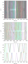 |
Fig. 1 Evolution of the value of the relative mean longitude, λr, of 2013 VZ70 with respect to Saturn. The results corresponding to the nominal orbit are shown in black, and the results of control orbits with Cartesian vectors separated by +1σ (in red), −1σ (in orange), +3σ (in green), −3σ (in cyan), +9σ (in purple), and −9σ (in violet) from the nominal values are also displayed. The output time-step size is 0.5 yr. The three panels show different time ranges to make the visualization easier. The input data (Cartesian vectors for all the Solar System objects) have JPL’s SBDB as a source and are referred to epoch 2459396.5 Barycentric Dynamical Time, which is also the origin of time in the calculations. |
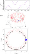 |
Fig. 2 Future horseshoe behavior for the nominal orbit. Top panel: future evolution of the value of the relative mean longitude, λr, with respect to Saturn for the nominal orbit of 2013 VZ70. Middle panel: Trajectory in three-dimensional space during the time interval (0, 800) yr in a frame of reference centered on the Sun and rotating with Saturn. Bottom panel: the path followed by 2013 VZ70 (which moves counterclockwise) is in a frame of reference centered on the Sun and rotating with Saturn, projected onto the ecliptic plane, during the same time interval. Since Saturn follows an eccentric orbit, it is represented in the panels by a blue trace (middle) or ellipse (bottom). The output time-step size is 0.01 yr. |
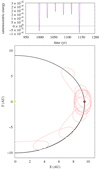 |
Fig. 3 Top panel: evolution of the Keplerian Saturnocentric energy of 2013 VZ70. Satellite captures happen when the relative binding energy becomes negative. The unit of energy is such that the unit of mass is 1 M⊙, the unit of distance is 1 AU, and the unit of time is one sidereal year divided by 2π. Bottom panel: path followed by 2013 VZ70 (which moves counterclockwise) in a frame of reference centered on the Sun (in yellow) and rotating with Saturn (in brown, its orbit in black), projected onto the ecliptic plane, during the time interval (950, 1200) yr, shown in pink. The output time-step size is 0.01 yr. |
4 Discussion
Alexandersen et al. (2018, 2020, 2021) favor an origin for 2013 VZ70 in the trans-Neptunian populations. One of Saturn’s irregular moons, Phoebe, is believed to be a captured centaur with a trans-Neptunian origin (see for example Johnson & Lunine 2005; Jewitt & Haghighipour 2007). Although such an origin is indeed possible, here we argue that the hostile resonant environment characteristic of Saturn’s neighborhood favors a scenario of in situ formation via impact, fragmentation, or tidal disruption within the population of irregular moons as 2013 VZ70 can experience encounters with Saturn at very low relative velocity (see above). Supporting arguments for a scenario of in situ formation come from two sides. In both cases, we used a relevant sample of natural satellites of Saturn. Given the fact that the orbit determinations of some moons of Saturn are somewhat poor and that their uncertainties are far from well characterized, we initially restricted our statistical analyses to the nominal orbits.
Heliocentric Keplerian orbital elements of Saturnian moons with e < 0.25.
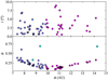 |
Fig. 4 Color-coded clusters generated by the k-means++ algorithm applied to the data set made of 64 Saturnian moons. The figure shows the heliocentric values (a, e, i). The range ini has been restricted to the one relevant to this work. Heliocentric Keplerian orbital elements refer to epoch JD 2459396.5. Source: JPL’s SBDB and Horizons. |
4.1 Natural satellites of Saturn: Orbital context
We retrieved the heliocentric orbital elements of the known natural satellites of Saturn from JPL’s SBDB for the epoch JD 2459396.5. Our sample included 64 moons with heliocentric e < 1 and a < 20 AU. The subsample with e < 0.25 is shown in Table 2. Figure 4 shows the result of applying the k-means algorithm and the elbow method to the data set of Saturn’s moon. Three clusters are found: The plum and fuchsia points include members of the Inuit and Gallic groups that follow Saturnocentric prograde orbits as well as members of the Norse group that follow Saturnocentric retrograde orbits (see Table 2), and the azure points include inner moons such as Atlas, Pan, and Polydeuces, but also Rhea (not shown in the top panel).
Table 2 shows that the heliocentric orbital elements of multiple irregular moons of Saturn resemble those of 2013 VZ70 in Table 1. However, most moons with provisional designations may correspond to lost objects that may have to be rediscovered (see for example Jacobson et al. 2012). Therefore, and among the moons in Table 2, we would like to single out Tarqeq and Siarnaq. Tarqeq (originally named S/2007 S 1 or Saturn LII; Sheppard et al. 2007a,b) has a size ofabout 6 km (Denk & Mottola 2019) and is a member of the Inuit group of irregular satellites of Saturn that also follow a low-eccentricity, low-inclination heliocentric orbit (see Table 2), like 2013 VZ70. Another object with similar orbital properties is Siarnaq (originally named S/2000 S 3 or Saturn XXIX; Gladman et al. 2000; Holman et al. 2001), which is the largest member of the Inuit group of Saturnian satellites, at about 39 km (Grav et al. 2015), and one of the fastest rotators, with a period of 10 h (Denk & Mottola 2019).
Centaur 2013 VZ70 could be similar in size to Tarqeq and other irregular satellites of Saturn, and its heliocentric orbit is consistent in terms of e and i with those of other moons. We interpret these facts as supportive of an origin among one of the groups of irregular satellites of Saturn.
4.2 Saturnian moons versus 2013 VZ70: Relative nodal distances
We computed the distribution of the absolute values of the mutual nodal distances of 2013 VZ70 and the sample of Saturnian moons using Eqs. (16) and (17) from Saillenfest et al. (2017) – Δ+ for the ascending nodes and Δ− for the descending nodes – and data from JPL’s SBDB and Horizons referred to epoch JD 2459396.5. Our results are shown in Fig. 5, and they indicate that the heliocentric orbits of some irregular satellites of Saturn pass rather close to the trajectory of 2013 VZ70. The first percentile of the distribution of Δ+ is 0.062 AU, and the mutual nodal distance between the ascending nodes of 2013 VZ70 and Thrymr is 0.058 AU. On the other hand, the first percentile of the distribution of Δ− is 0.059 AU, and the mutual nodal distance between the descending nodes of 2013 VZ70 and Fornjot is 0.015 AU. Both cases are clear outliers.
Thrymr and Fornjot are members of the Norse group (see Table 2) of irregular satellites of Saturn that follow Saturnocentric retrograde orbits. Thrymr (originally named S/2000 S 7 or Saturn XXX; Petit et al. 2001) is believed to be debris released during an impact on Phoebe (Denk & Mottola 2019). Fornjot (originally named S/2004 S 8 or Saturn XLII; Jewitt et al. 2006)is one of the outermost natural satellites of Saturn and also one of the fastest rotators, with a period of 7 or 9.5 h (Denk & Mottola 2019).
We interpret the existence of these low probability, short mutual nodal distances as an indication of a collisional origin for 2013 VZ70. However, for a given pair of objects, a present-day short mutual nodal distance does not imply an equally short value in the past or the future. In addition, although it is true that close flybys take place in the vicinity of the mutual nodes, short mutual nodal distances may not translate into actual flybys if there are active protection mechanisms such as mean-motion or secular resonances like in the cases of Neptune’s trojans or Pluto (see for example Milani et al. 1989; Wan et al. 2001).
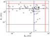 |
Fig. 5 Distribution of mutual nodal distances (Δ+, ascending; Δ−, descending) between 2013 VZ70 and a sample of Saturn satellites. The median values are shown in blue and the 1st and 99th percentiles in red. |
4.3 Possible past encounters of 2013 VZ70 with Fornjot and Thrymr
The present-day short mutual nodal distances of 2013 VZ70 and Fornjotand Thrymr are indicative of a possible past collisional evolution of 2013 VZ70. The assessment of the concurrent past orbital evolution of 2013 VZ70 and Fornjot and Thrymr should be based on the statistical analysis of results from a representative sample of N-body simulations. Unfortunately, in this case the effect of the uncertainties is not easy to include in the calculations.
The current orbit determination of 2013 VZ70 in Table 1 is based on data collected for less than 10% of its sidereal orbital period. Although it can certainly be improved, the relative errors in the orbital elements are in the range 10−4–10−5, and this makes any short-term ephemerides (for example, present-day Cartesian state vectors) computed from it reasonably robust. However, this centaur moves in a very unstable region, and the results presented in Sect. 3 indicate that control orbits relatively close to the nominal one lead to a rather different orbital evolution both into the past and forward in time outside the time interval (−1000, 1000) yr. In sharp contrast, the orbit determinations of known irregular moons of Saturn have uncertainties affected by poorly characterized systematics present in sparse observation sets. Figure 1 in Jacobson et al. (2012) shows that the on-sky position uncertainty of these irregular moons may oscillate over time. Table 3 in Jacobson et al. (2012) shows that this uncertainty could be as high as 0.′′7 and 5.′′7 for Thrymr and Fornjot, respectively, after three orbital periods beyond 2012 January. In such cases, there is no reliable procedure for computing meaningful 1σ uncertainties for a given set of barycentric Cartesian state vectors.
The planetary satellite ephemeris SAT368 computed by RA Jacobson in 2014 updated the irregular satellites of Saturn with Earth-based data through early 2014 and all Cassini imaging through 2013, and they are utilized by Horizons to provide Cartesian state vectors that can be used as input data to perform the required N-body simulations. Horizons cannot provide estimates of the associated 1σ uncertainties, but the barycentric Cartesian state vectors are shown in Tables A.2 and A.3. We used a sample of 1500 pairs of Gaussian-distributed control orbits (see Appendix A) based on the Cartesian vectors in Tables A.1 and A.2 and integrated backwards in time for 1500 yr (assuming uncertainties of 10% and 5% for Fornjot), considering the same physical model used in Sect. 3 (in this simplified set of experiments, the contribution of massive moons was neglected), and studied the distribution of minimum approach distances (see de la Fuente Marcos et al. 2021b for additional details on this approach).
Figure 6 shows that flybys as close as 0.011 AU are possible, a result fully consistent with the one obtained in the previous section for the distribution of mutual nodal distances. Our results also show that by considering smaller uncertainties in the case of Fornjot, the minimum approach distance decreases. Figure 7 shows equivalent results for Thrymr, and flybys as close as 0.016 AU are possible. These results, based on N-body calculations, confirm that 2013 VZ70 may have approached Fornjot and Thrymr at relatively short range in the past, despite us using a rather conservative choice when factoring uncertainties into the calculations. Lowering the level of uncertainty may produce flybys an order of magnitude or two closer. In addition, our flyby experiments show that the brief periods of capture of 2013 VZ70 as a temporary irregular moon of Saturn are ubiquitous.
As an additional quality control step, we repeated the experiment (600 instances), focusing on encounters between the moons Fornjot and Thrymr. Figure 8 shows that flybys as close as 0.0007 AU are possible when assuming uncertainties of 5%.
5 Summary and conclusions
In this work, we have studied the orbital evolution of 2013 VZ70 backward and forward in time using direct N-body simulations and factoring the uncertainties into the calculations. We have also explored a possible connection between 2013 VZ70 and the moons of Saturn by computing the distribution of mutual nodal distances between this centaur and a sample of moons to investigate how close two orbits can get to each other. Our conclusions can be summarized as follows:
- 1.
We show that 2013 VZ70 is a present-day co-orbital to Saturn of the horseshoe type. It is, however, a transient co-orbital;
- 2.
Centaur 2013 VZ70 may approach Saturn at very low relative velocity; as a result, it might experience brief periods of capture as a temporary irregular moon;
- 3.
The orbit of 2013 VZ70 is similar in terms of eccentricity and inclination to the Inuit group of irregular moons of Saturn, particularly Siarnaq and Tarqeq;
- 4.
The analysis of the distribution of mutual nodal distances between 2013 VZ70 and a sample of moons shows that the mutual nodal distance for the descending nodes of this centaur and Fornjot is 0.015 AU and that for the ascending nodes of the object and Thrymr is 0.058 AU. In both cases, the values are below the first percentile of the distribution;
- 5.
The orbit determination of 2013 VZ70 still requires significant improvement. Any prediction beyond the time interval (−1000, 1000) yr based on the orbit determination in Table 1 is very uncertain. The available data cannot be used to confirm or reject an origin for 2013 VZ70 in the trans-Neptunian populations or within the groups of irregular moons of Saturn, which have in some cases even more uncertain orbit determinations.
The facts are that (i) 2013 VZ70 might pass fairly close (as confirmed with N-body calculations) to some of the moons of the Norse group that could be debris from Phoebe (Denk & Mottola 2019), (ii) its orbit is similar to the heliocentric orbits of some of the moons of the Inuit group (see Tables 1 and 2), and (iii) it also can approach Saturn at low relative velocity, sufficiently low to become a temporary moon itself, as discussed in Sect. 3. These three objective pieces of information are supportive of a scenario of in situ formation via impact, fragmentation, or tidal disruption within the population of the irregular moons of Saturn. The orbital evolution analysis in Sect. 3 suggests that the putative formation event may have taken place relatively recently or, because predictions are very uncertain, more than about 1000 yr ago.
On the other hand, if 2013 VZ70 is debris linked to Phoebe, which is believed to be a captured object with an origin in trans-Neptunian space (see for example Johnson & Lunine 2005; Jewitt & Haghighipour 2007 but also consider Castillo-Rogez et al. 2019), spectroscopic studies may not be able to confirm or refute its putative origin, captured versus collisional. It is possible that only improvements in the orbit determinations of 2013 VZ70 and the population of irregular moons of Saturn will eventually lead to a robust solution of this dilemma.
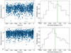 |
Fig. 6 Distribution of minimum approach distances for the pair 2013 VZ70 and Fornjot. Top panels: assuming uncertainties of 10% for the barycentric Cartesian state vector of Fornjot in Table A.2. Bottom panels: assuming uncertainties of 5%. The median values are shown as vertical green lines. |
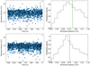 |
Fig. 7 Distribution of minimum approach distances for the pair 2013 VZ70 and Thrymr. Top panels: assuming uncertainties of 10% for the barycentric Cartesian state vector of Thrymr in Table A.3. Bottom panels: assuming uncertainties of 5%. The median values are shown as vertical green lines. |
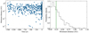 |
Fig. 8 Distribution of minimum approach distances for the pair Fornjot and Thrymr. Our calculations assumed uncertainties of 5%. The median values are shown as vertical green lines. |
Acknowledgements
We thank the referee for her/his prompt report that included a very helpful suggestion regarding the interpretation of our results, S.J. Aarseth for providing one of the codes used in this research, A.B. Chamberlin for helping with the new JPL’s Solar System Dynamics website, J.D. Giorgini for comments and insight on the uncertainties of the orbit determinations of the irregular moons of Saturn, and A.I. Gómez de Castro for providing access to computing facilities. Part of the calculations and the data analysis were completed on the Brigit HPC server of the ‘Universidad Complutense de Madrid’ (UCM), andwe thank S. Cano Alsúa for his help during this stage. This work was partially supported by the Spanish ‘Ministerio de Economía y Competitividad’ (MINECO) under grant ESP2017-87 813-R. In preparation of this paper, we made use of the NASA Astrophysics Data System, the ASTRO-PH e-print server, and the MPC data server.
Appendix A Input data
Here, we include the barycentric Cartesian state vectors of the centaur 2013 VZ70 and the moons Fornjot and Thrymr. These vectors and their uncertainties (provided or assumed) were used to carry out the calculations discussed in the main text, to generate the figures that display the time evolution of the critical angle, and to generate the histograms and distributions of the close en- counters of pairs of objects. For example, a new value of the X component of the state vector is computed as Xc = X + σX r, where r is a univariate Gaussian random number and X and σX are the mean value and its 1σ uncertainty (provided or assumed) in the corresponding table.
Barycentric Cartesian state vector of 2013 VZ70: compo- nents and associated 1σ uncertainties.
Barycentric Cartesian state vector of Fornjot (originally named S/2004 S 8 or Saturn XLII): components.
Barycentric Cartesian state vector of Thrymr (originally named S/2000 S 7 or Saturn XXX): components.
References
- Aarseth, S. J. 2003, Gravitational N-Body Simulations (Cambridge: Cambridge University Press), 27 [Google Scholar]
- Alexandersen, M., Greenstreet, S., Gladman, B., et al. 2018, in AAS/Division for Planetary Sciences Meeting Abstracts, 50, 305.09 [NASA ADS] [Google Scholar]
- Alexandersen, M., Greenstreet, S., Gladman, B., et al. 2020, in AAS/Division for Planetary Sciences Meeting Abstracts, 52, 206.06 [NASA ADS] [Google Scholar]
- Alexandersen, M., Greenstreet, S., Gladman, B., et al. 2021, PSJ, 2, 212 [NASA ADS] [CrossRef] [Google Scholar]
- Ashton, E., Gladman, B., & Beaudoin, M. 2021, PSJ, 2, 158 [NASA ADS] [Google Scholar]
- Bannister, M. T., Kavelaars, J. J., Petit, J.-M., et al. 2016, AJ, 152, 70 [NASA ADS] [CrossRef] [Google Scholar]
- Bannister, M. T., Kavelaars, J. J., Gladman, B. J., et al. 2021, Minor Planet Electronic Circulars, 2021-Q55 [Google Scholar]
- Castillo-Rogez, J., Vernazza, P., & Walsh, K. 2019, MNRAS, 486, 538 [CrossRef] [Google Scholar]
- de la Barre, C. M., Kaula, W. M., & Varadi, F. 1996, Icarus, 121, 88 [NASA ADS] [CrossRef] [Google Scholar]
- de la Fuente Marcos, C., & de la Fuente Marcos, R. 2012, MNRAS, 427, 728 [Google Scholar]
- de la Fuente Marcos, C., & de la Fuente Marcos, R. 2016, MNRAS, 462, 3344 [Google Scholar]
- de la Fuente Marcos, C. & de la Fuente Marcos, R. 2021a, MNRAS, 501, 6007 [NASA ADS] [CrossRef] [Google Scholar]
- de la Fuente Marcos, C., de la Fuente Marcos, R., Licandro, J., et al. 2021b, A&A, 649, A85 [NASA ADS] [CrossRef] [EDP Sciences] [Google Scholar]
- Denk, T., & Mottola, S. 2019, Icarus, 322, 80 [CrossRef] [Google Scholar]
- Dermott, S. F., & Murray, C. D. 1981, Icarus, 48, 12 [NASA ADS] [CrossRef] [Google Scholar]
- Everhart, E. 1973, AJ, 78, 316 [NASA ADS] [CrossRef] [Google Scholar]
- Fedorets, G., Granvik, M., & Jedicke, R. 2017, Icarus, 285, 83 [Google Scholar]
- Freedman, D., & Diaconis, P. 1981, Zeitschrift für Wahrscheinlichkeitstheorie und Verwandte Gebiete, 57, 453 [CrossRef] [Google Scholar]
- Gallardo, T. 2006, Icarus, 184, 29 [Google Scholar]
- Ginsburg, A., Sipőcz, B. M., Brasseur, C. E., et al. 2019, AJ, 157, 98 [Google Scholar]
- Giorgini, J. 2011, in Journées Systèmes de Référence Spatio-temporels 2010, ed. N. Capitaine, 87 [Google Scholar]
- Giorgini, J. D. 2015, IAUGA, 22, 2256293 [Google Scholar]
- Gladman, B., Kavelaars, J., Allen, R. L., et al. 2000, IAU Circ., 7513 [Google Scholar]
- Grav, T., Bauer, J. M., Mainzer, A. K., et al. 2015, ApJ, 809, 3 [NASA ADS] [CrossRef] [Google Scholar]
- Harris, C. R., Millman, K. J., van der Walt, S. J., et al. 2020, Nature, 585, 357 [NASA ADS] [CrossRef] [Google Scholar]
- Holman, M., Gladman, B., Grav, T., et al. 2001, Minor Planet Electronic Circulars, 2001-U42 [Google Scholar]
- Hou, X. Y., Scheeres, D. J., & Liu, L. 2014, MNRAS, 437, 1420 [NASA ADS] [CrossRef] [Google Scholar]
- Huang, Y., Li,M., Li, J., et al. 2019, MNRAS, 488, 2543 [NASA ADS] [CrossRef] [Google Scholar]
- Hunter, J. D. 2007, Comput. Sci. Eng., 9, 90 [NASA ADS] [CrossRef] [Google Scholar]
- Innanen, K. A., & Mikkola, S. 1989, AJ, 97, 900 [NASA ADS] [CrossRef] [Google Scholar]
- Ito, T., & Tanikawa, K. 1999, Icarus, 139, 336 [NASA ADS] [CrossRef] [Google Scholar]
- Ito, T., & Tanikawa, K. 2002, MNRAS, 336, 483 [NASA ADS] [CrossRef] [Google Scholar]
- Jacobson, R., Brozović, M., Gladman, B., et al. 2012, AJ, 144, 132 [NASA ADS] [CrossRef] [Google Scholar]
- Jedicke, R., Bolin, B. T., Bottke, W. F., et al. 2018, Front. Astron. Space Sci., 5, 13 [CrossRef] [Google Scholar]
- Jewitt, D., & Haghighipour, N. 2007, ARA&A, 45, 261 [NASA ADS] [CrossRef] [Google Scholar]
- Jewitt, D. C., Sheppard, S. S., Kleyna, J., et al. 2006, Minor Planet Electronic Circulars, 2006-C74 [Google Scholar]
- Johnson, T. V., & Lunine, J. I. 2005, Nature, 435, 69 [NASA ADS] [CrossRef] [Google Scholar]
- Li, M., Huang, Y., & Gong, S. 2018, A&A, 617, A114 [NASA ADS] [CrossRef] [EDP Sciences] [Google Scholar]
- Makino, J. 1991, ApJ, 369, 200 [Google Scholar]
- Marzari, F., Tricarico, P., & Scholl, H. 2002, ApJ, 579, 905 [NASA ADS] [CrossRef] [Google Scholar]
- Melita, M. D., & Brunini, A. 2001, MNRAS, 322, L17 [NASA ADS] [CrossRef] [Google Scholar]
- Mikkola, S., Innanen, K., Wiegert, P., et al. 2006, MNRAS, 369, 15 [NASA ADS] [CrossRef] [Google Scholar]
- Milani, A., Nobili, A. M., & Carpino, M. 1989, Icarus, 82, 200 [Google Scholar]
- Morais, M. H. M., & Namouni, F. 2013a, Celest. Mech. Dyn. Astron., 117, 405 [NASA ADS] [CrossRef] [Google Scholar]
- Morais, M. H. M., & Namouni, F. 2013b, MNRAS, 436, L30 [Google Scholar]
- Morais, H., & Namouni, F. 2017, Nature, 543, 635 [NASA ADS] [CrossRef] [Google Scholar]
- Morais, M. H. M., & Namouni, F. 2019, MNRAS, 490, 3799 [CrossRef] [Google Scholar]
- Murray, C. D., & Dermott, S. F. 1999, Solar System Dynamics (Cambridge: Cambridge University Press) [Google Scholar]
- Musen, P. 1971, NASA Tech. Note, 6279 [Google Scholar]
- Namouni, F. 1999, Icarus, 137, 293 [NASA ADS] [CrossRef] [Google Scholar]
- Namouni, F., & Murray, C. D. 2000, Celest. Mech. Dyn. Astron., 76, 131 [NASA ADS] [CrossRef] [Google Scholar]
- Namouni, F., Christou, A. A., & Murray, C. D. 1999, Phys. Rev. Lett., 83, 2506 [NASA ADS] [CrossRef] [Google Scholar]
- Nesvorný, D., & Dones, L. 2002, Icarus, 160, 271 [CrossRef] [Google Scholar]
- Pedregosa, F., Varoquaux, G., Gramfort, A., et al. 2011, J. Mach. Learn. Res., 12, 2825 [Google Scholar]
- Petit, J.-M., Nicholson, P., Dumas, C., et al. 2001, Minor Planet Electronic Circulars, 2001-X20 [Google Scholar]
- Saillenfest, M., Fouchard, M., Tommei, G., et al. 2017, Celest. Mech. Dyn. Astron., 129, 329 [Google Scholar]
- Sheppard, S. S., Jewitt, D. C., Kleyna, J., et al. 2007a, IAU Circ., 8836 [Google Scholar]
- Sheppard, S. S., Jewitt, D. C., Kleyna, J., et al. 2007b, Minor Planet Electronic Circulars, 2007-G38 [Google Scholar]
- Sidorenko, V. V. 2020, AJ, 160, 257 [NASA ADS] [CrossRef] [Google Scholar]
- Sidorenko, V. V., Neishtadt, A. I., Artemyev, A. V., et al. 2014, Celest. Mech. Dyn. Astron., 120, 131 [NASA ADS] [CrossRef] [Google Scholar]
- Tanikawa, K., & Ito, T. 2007, PASJ, 59, 989 [NASA ADS] [Google Scholar]
- Turrini, D., Marzari, F., & Beust, H. 2008, MNRAS, 391, 1029 [NASA ADS] [CrossRef] [Google Scholar]
- Turrini, D., Marzari, F., & Tosi, F. 2009, MNRAS, 392, 455 [CrossRef] [Google Scholar]
- van der Walt, S., Colbert, S. C., & Varoquaux, G. 2011, Comput. Sci. Eng., 13, 22 [Google Scholar]
- Wan, X.-S., Huang, T.-Y., & Innanen, K. A. 2001, AJ, 121, 1155 [Google Scholar]
- Wiegert, P., Innanen, K., & Mikkola, S. 2000, AJ, 119, 1978 [NASA ADS] [CrossRef] [Google Scholar]
- Zink, J. K., Batygin, K., & Adams, F. C. 2020, AJ, 160, 232 [NASA ADS] [CrossRef] [Google Scholar]
All Tables
Barycentric Cartesian state vector of 2013 VZ70: compo- nents and associated 1σ uncertainties.
Barycentric Cartesian state vector of Fornjot (originally named S/2004 S 8 or Saturn XLII): components.
Barycentric Cartesian state vector of Thrymr (originally named S/2000 S 7 or Saturn XXX): components.
All Figures
|
Fig. 1 Evolution of the value of the relative mean longitude, λr, of 2013 VZ70 with respect to Saturn. The results corresponding to the nominal orbit are shown in black, and the results of control orbits with Cartesian vectors separated by +1σ (in red), −1σ (in orange), +3σ (in green), −3σ (in cyan), +9σ (in purple), and −9σ (in violet) from the nominal values are also displayed. The output time-step size is 0.5 yr. The three panels show different time ranges to make the visualization easier. The input data (Cartesian vectors for all the Solar System objects) have JPL’s SBDB as a source and are referred to epoch 2459396.5 Barycentric Dynamical Time, which is also the origin of time in the calculations. |
| In the text | |
|
Fig. 2 Future horseshoe behavior for the nominal orbit. Top panel: future evolution of the value of the relative mean longitude, λr, with respect to Saturn for the nominal orbit of 2013 VZ70. Middle panel: Trajectory in three-dimensional space during the time interval (0, 800) yr in a frame of reference centered on the Sun and rotating with Saturn. Bottom panel: the path followed by 2013 VZ70 (which moves counterclockwise) is in a frame of reference centered on the Sun and rotating with Saturn, projected onto the ecliptic plane, during the same time interval. Since Saturn follows an eccentric orbit, it is represented in the panels by a blue trace (middle) or ellipse (bottom). The output time-step size is 0.01 yr. |
| In the text | |
|
Fig. 3 Top panel: evolution of the Keplerian Saturnocentric energy of 2013 VZ70. Satellite captures happen when the relative binding energy becomes negative. The unit of energy is such that the unit of mass is 1 M⊙, the unit of distance is 1 AU, and the unit of time is one sidereal year divided by 2π. Bottom panel: path followed by 2013 VZ70 (which moves counterclockwise) in a frame of reference centered on the Sun (in yellow) and rotating with Saturn (in brown, its orbit in black), projected onto the ecliptic plane, during the time interval (950, 1200) yr, shown in pink. The output time-step size is 0.01 yr. |
| In the text | |
|
Fig. 4 Color-coded clusters generated by the k-means++ algorithm applied to the data set made of 64 Saturnian moons. The figure shows the heliocentric values (a, e, i). The range ini has been restricted to the one relevant to this work. Heliocentric Keplerian orbital elements refer to epoch JD 2459396.5. Source: JPL’s SBDB and Horizons. |
| In the text | |
|
Fig. 5 Distribution of mutual nodal distances (Δ+, ascending; Δ−, descending) between 2013 VZ70 and a sample of Saturn satellites. The median values are shown in blue and the 1st and 99th percentiles in red. |
| In the text | |
|
Fig. 6 Distribution of minimum approach distances for the pair 2013 VZ70 and Fornjot. Top panels: assuming uncertainties of 10% for the barycentric Cartesian state vector of Fornjot in Table A.2. Bottom panels: assuming uncertainties of 5%. The median values are shown as vertical green lines. |
| In the text | |
|
Fig. 7 Distribution of minimum approach distances for the pair 2013 VZ70 and Thrymr. Top panels: assuming uncertainties of 10% for the barycentric Cartesian state vector of Thrymr in Table A.3. Bottom panels: assuming uncertainties of 5%. The median values are shown as vertical green lines. |
| In the text | |
|
Fig. 8 Distribution of minimum approach distances for the pair Fornjot and Thrymr. Our calculations assumed uncertainties of 5%. The median values are shown as vertical green lines. |
| In the text | |
Current usage metrics show cumulative count of Article Views (full-text article views including HTML views, PDF and ePub downloads, according to the available data) and Abstracts Views on Vision4Press platform.
Data correspond to usage on the plateform after 2015. The current usage metrics is available 48-96 hours after online publication and is updated daily on week days.
Initial download of the metrics may take a while.