| Issue |
A&A
Volume 657, January 2022
|
|
|---|---|---|
| Article Number | A29 | |
| Number of page(s) | 13 | |
| Section | Stellar atmospheres | |
| DOI | https://doi.org/10.1051/0004-6361/202140947 | |
| Published online | 22 December 2021 | |
Sulfur abundances in the Galactic bulge and disk★
1
Departamento de Ciencias Fisicas, Universidad Andres Bello,
Fernandez Concha 700,
Las Condes,
Santiago, Chile
e-mail: This email address is being protected from spambots. You need JavaScript enabled to view it.
2
GEPI, Observatoire de Paris, Université PSL, CNRS, Place Jules Janssen,
92195
Meudon, France
3
Dipartimento di Fisica e Astronomia, Università degli Studi di Bologna,
Via Gobetti 93/2,
40129
Bologna, Italy
4
INAF – Osservatorio di Astrofisica e Scienza dello Spazio di Bologna,
Via Gobetti 93/3,
40129
Bologna, Italy
Received:
31
March
2021
Accepted:
9
September
2021
Abstract
Context. The measurement of α-element abundances provides a powerful tool for placing constraints on the chemical evolution and star formation history of galaxies. The majority of studies on the α-element sulfur (S) are focused on local stars, making S behavior in other environments an astronomical topic that is yet to be explored in detail.
Aims. The investigation of S in the Galactic bulge was recently considered for the first time. This work aims to improve our knowledge on S behavior in this component of the Milky Way.
Methods. We present the S abundances of 74 dwarf and sub-giant stars in the Galactic bulge, along with 21 and 30 F and G thick- and thin-disk stars, respectively. We performed a local thermodynamic equilibrium analysis and applied corrections for non-LTE on high resolution and high signal-to-noise UVES spectra. S abundances were derived from multiplets 1, 6, and 8 in the metallicity range of − 2 < [Fe/H] < 0.6, by spectrosynthesis or line equivalent widths.
Results. We confirm that the behavior of S resembles that of an α-element within the Galactic bulge. In the [S/Fe] versus [Fe/H] diagram, S presents a plateau at low metallicity, followed by a decreasing of [S/Fe] with the increasing of [Fe/H], before reaching [S/Fe] ~ 0 at a super-solar metallicity. We found that the Galactic bulge is S-rich with respect to both the thick- and thin-disks at − 1 < [Fe/H] < 0.3, supporting a scenario of more rapid formation and chemical evolution in the Galactic bulge than in the disk.
Key words: stars: abundances / Galaxy: bulge / Galaxy: disk
This paper is based on data collected with the Very Large Telescope (VLT) at the European Southern Observatory (ESO) on Paranal, Chile (ESO Program ID 065.L-0507, 071.B-0529, 076.B-0055, 076.B-0133, 077.B-0507, 079.D-0567, 082.B-0453, 083.B-0265, 084.B-0837, 084.D-0965, 085.B-0399, 086.B-0757, 087.B-0600, 087.D-0724, 088.B-0349, 089.B-0047, 090.B-0204, 091.B-0289, 092.B-0626, 093.B-0700, 094.B-0282, 165.L-0263, 167.D-0173, 266.D-5655; and data from the UVES Paranal Observatory Project (ESO DDT Program ID 266.D-5655).
© ESO 2021
1 Introduction
The Galactic bulge (bulge) is one of the main, more massive, and older components of the Milky Way (MW). Despite the studies performed in the last 30 yr, both spectroscopic (McWilliam & Rich 1994; Rich et al. 2007; Ness & Freeman 2012; Rojas-Arriagada et al. 2014; Johnson et al. 2014; Zoccali et al. 2017) and photometric (Clarkson et al. 2008; Gennaro et al. 2015; Renzini et al. 2018), the formation and the evolution of bulge is still an open issue. Kormendy & Kennicutt (2004) classified local bulges into classical and pseudo-bulges. From the morphological point of view, classical bulges are more spheroidal and massive with respect to disks. Their shape suggests that they were created from gravitational collapse of primordial gas (Eggen et al. 1962; Matteucci & Brocato 1990) or by hierarchical merging of smaller structures (Blumenthal et al. 1984). According to this theory, classical bulges formed during the first phase of galaxy formation, making them older than disks. On the other hand, pseudo-bulges are associated with bars and smaller disk-like structures. Their origin is due to the secular evolution of disks. In particular, the internal instabilities of the disk bring gas and stars into the central regions of the galaxy, building up the bulge (Athanassoula 2005; Genzel et al. 2008). Nowadays, the notion that more than one scenario is involved in the formation of bulges is strongly supported (Robertson et al. 2006; Bournaud et al. 2009; Rahimi et al. 2010).
Since the Galactic bulge is the only bulge that can be resolved into individual stars, it represents a unique laboratory with which to understand the formation and evolution of bulges and their galaxies. The analysis of bulge stars contributes to establishing constraints on the formation timescales and chemical enrichment of the earliest stellar populations in the galaxy. In particular, the chemical evolution and the star formation history (SFH) of the bulge can be derived from measured abundance ratios.
The α-elements and iron-peak elements play a fundamental role in this context since their nucleosynthesis occurs on different timescales. While α-elements are produced by Type II Supernovae (SNe) on a timescale of ~30 Myr, iron-peak elements are produced by Type Ia SNe on longer timescales (>1–2 Gyr). Thus, the investigation of the α-elements behavior in the bulge is a crucial topic for our understanding of its formation and evolution.
Rich & Origlia (2005) measured α-elements (O, Mg, Si, Ca, Ti) abundances in 14 M giant stars belonging to the bulge, in the metallicity range − 0.35 < [Fe/H] < 0, using infra-red spectra. Overall, they found an α-enhancement of approximately +0.3 dex in bulge stars with respect to the local disk. Using high resolution UVES spectra, Zoccali et al. (2008) measured O, Na, Mg, and Al abundances for 50 K giants in the bulge. In the metallicity range of − 0.8 < [Fe/H] < 0.4, they obtained [O/Fe] and [Mg/Fe] bulge trends higher than those measured in both thin- and thick-disk stars. Taking advantage of microlensing events, in a series of papers, Bensby and collaborators (2013, 2017, 2020) spectroscopically characterized the bulge by studying dwarf and sub-giant stars. Among the 13 species considered, they measured the Mg, Si, Ca, and Ti abundances and found that the level of α-enhancement is slightly higher in the bulge than in the thick-disk. Moreover, the bulge presents a knee in the [α/Fe] trend located at ~0.1 dex higher [Fe/H] than in the local thick-disk. It should be noted that while all the stars studied by Bensby and collaborators lie in the direction of the bulge, they are not necessarily well-established members of the bulge. Thus, all these studies have concluded that the bulge formed before and more rapidly than the disk.
On the other hand, Meléndez et al. (2008) measured O abundances from high resolution near-infrared (NIR) spectra of 19 bulge giant stars and found no chemical distinction between the bulge and the local thick-disk at [Fe/H] < −0.2. They analyzed the formation timescales, star formation rate, and initial mass function of bulge and disk to argue the similar chemical evolution of these components of the MW. Similar results were obtained for three K bulge giant stars by Ryde et al. (2009). According to this work, the O abundances measured from high-resolution NIR spectra in bulge and thick-disk stars are similar. The similarity between the bulge and thick-disk trends was also confirmed by Gonzalez et al. (2011, 2015), who measured Mg, Ca, Ti, and Si abundances from high-resolution (R) and high signal-to-noise ratio (S/N) FLAMES/GIRAFFE spectra of bulge giants.
Recently, Griffith et al. (2021) investigated the similarity or dissimilarity between the chemical trends of Apache Point Observatory Galactic Evolution Experiment (APOGEE, Majewski et al. 2017) bulge (RGC < 3 kpc) and thick-disk (5 kpc < RGC < 11 kpc) stars. Dividing bulge and thick-disk stars in low-Ia (high-[Mg/Fe]) and high-Ia (low-[Mg/Fe]) populations, they measured chemical abundances of seventeen species to analyze the median trend in the [X/Mg] vs. [Mg/H] plane. They found nearly identical median trends for low-Ia thick-disk and bulge stars for all elements, while the high-Ia trends are similar for most elements except Mn, Na, and Co. Obtaining typical differences ≲ 0.03 dex between the abundance trends, Griffith et al. (2021) concluded that bulge and thick-disk were enriched by similar nucleosynthetic processes.
Among the different α-elements, sulfur has not been thoroughly studied. Sulfur (S) is produced in the final stage of the evolution of massive stars (M* > 20M⊙). The hydrostatic burning of neon (Ne), at the core temperature log Tc = 9.09 K, leads to the formation of an oxygen (O) convective core and the production of α-elements up to 32S. Once log Tc = 9.5 K is reached, the oxygen burning phase starts producing 28Si, 32S, and 34S. This amount of sulfur will be almost completely destroyed during the Si burning phase at 2.3 × 10⁹ K, so it will not contribute to the gas forming the next generation of stars. However, the production of S continues in the O convective shell burning in upper layers and it is provided also by explosive O burning during type II SNe explosion (Limongi & Chieffi 2003; Kobayashi et al. 2020). Unlike other α-elements, S is moderately volatile. For this reason, its abundance measured in stars in the Local Group galaxies canbe directly compared to those measured in extra-galactic HII regions or damped Ly-α systems (DLA). Hence, S abundances (A(S)) provide clues on the SFH and on properties of the interstellar medium (ISM), connecting the local and distant Universe. In the stellar spectra, there are a few S multiplets (Mult.) available. In the optical range there are Mult. 1, 6, and 8 at 920, 870, and 675 nm, respectively. Then, the Mult. 3 at 1045 nm and a forbidden line [SI] (1082 nm) lie in the NIR part of the spectra. Mult. 6 and 8 features are useful for solar metallicity or slightly metal-poor stars. However, these lines are weak, sohigh-resolution and high S/N spectra are required to make use of them. The strongest features of S are those of Mult. 1 and 3, allowing us to investigate A(S) in the metal-poor regime. The analysis of solar-metallicity dwarf stars and metal-poor giants can be carried out from the line [SI] at 1082 nm. On the other hand, these lines are located in a spectral range strongly contaminated by telluric absorptions. For these reasons, the study of S is often omitted in favor of the easier analysis of other α-elements. As a result, our knowledge about the behavior of S is still poor with respect to that of other α-elements.
This is particularly true when we consider the Galactic bulge. Indeed, A(S) have only recently been measured for the first time in this component of the MW by Griffith et al. (2021) using the S I lines at 15 478.5 and 16 576.6 Å, measured on high resolution NIR APOGEE spectra of red giant branch (RGB) stars. In this work, we present new S abundances in dwarf and sub-giant branch (SGB) stars belonging to the bulge and the disk based on high resolution, high S/N archival optical spectra, using the multiplets 1, 6, and 8 and we compare ours with literature results.
The paper is structured as follows: the used data sets are described in Sect. 2. In Sect. 3, we explain the analysis and the method adopted to obtain the A(S). We compare our results with those in the literature in Sect. 4. Finally, our conclusions are given in Sect. 5.
2 Observational data
Considering the distance of the bulge and the high degree of interstellar extinction in the Galactic plane, giant stars are the best tracers for the bulge. However, all the S lines we use are of high excitation so they become weak in cool stars. For this reason, dwarf stars can be considered among the best tracers of Galactic chemical evolution of S.
The faintness of bulge dwarf stars is the main difficulty in their observation. The high-resolution spectra of these stars can be obtained when a gravitational micro-lensing event occurs, during which the star may brighten by factors of hundreds. Several bulge dwarfs and sub-giant stars have been observed during microlensing events (Bensby et al. 2009, 2010a, 2010b, 2011, 2013, 2017, 2020). On these occasions, from 2 to 8 ~1800 s UVES (Dekker et al. 2000) exposures were recorded with a 0.7″ wide slit with wavelength coverage in the intervals 376–498 nm, 568–750 nm, and 766–946 nm. During the same night of observations, one rapidly rotating B star for each target was observed to evaluate the effect due to the Earth atmosphere. We retrieved the UVES-reduced (UVES pipeline version 5.10.131) data from the ESO data archive2. The reduced spectra are characterized by R = 42 310 and S∕N ~ 19–183 at ~921 nm. The coordinates and the S/N of the data are listed in Table A.1.
In order to minimize systematic errors, a homogeneous comparison between bulge and disk stars with atmospheric parameters that are estimated in a consistent way is required. Bensby et al. (2014) spectroscopically analyzed 714 F and G dwarf and subgiant stars in the nearby Galactic disk. Using kinematical criteria defined in Bensby et al. (2003), they obtained, for each star, two relative probabilities: the thick-disk-to-thin-disk (TD/D) and the thick-disk-to-halo (TD/H) membership. They required a probability of TD/D > 2 to classify a star as thick-disk candidate, while TD/D < 0.5 for a candidate thin-disk star. According to their kinematical criteria, their sample includes 387 stars with thin-disk kinematics, 203 stars with thick-disk kinematics, 36 stars with halo kinematics (TD/H < 1), and 89 starswith kinematics between those of thin- and thick-disks.
We explored the UVES archive searching for high resolution (R > 40 000) and high signal-to-noise (S∕N > 100) spectra for the sample of 203 thick-disk stars, in the wavelength range where S lines of Mults. 1, 6, and 8 are available. The reduced spectra of 23 thick-disk stars were found and retrieved for the analysis. The data are characterized by R ~ 42 000–110 000 and S∕N ~ 122–400 and they cover the wavelength range 665–1042 nm or 565–946 nm. In Table A.2, we report the names and coordinates of the thick-disk stars from the Hipparcos catalog (Perryman et al. 1997).
Among the 387 thin-disk stars (Bensby et al. 2014), 30 stars were observed during the UVES Paranal Observatory Project3 (UVES POP, Bagnulo et al. 2003). We obtained the UVES POP spectra, which cover the wavelength range 300–1000 nm and are characterized by R ~ 80 000 and S∕N ~ 300–500 in the V band. The names and coordinates of UVES POP stars are reported in Table A.3.
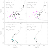 |
Fig. 1 log(g) versus log(Teff) diagrams of the stellar sample considered in this work. The bulge and the thick- and thin-disk stars are shown in black, cyan, and magenta respectively. The black filled circle and open circles are bulge dwarfs and giants. In each panel, we show the metallicities and the ages adopted to obtain isochrones from the Dartmouth Stellar Evolution Database (Dotter et al. 2008). |
3 Stellar sample analysis
The sample of stars considered in this work was already studied by Bensby et al. (2009, 2010a,b, 2011, 2013, 2014, 2017, 2020). These authors estimated the atmospheric parameters and chemical abundances of 13 species (Fe, O, Na, Mg, Al, Si, Ca, Ti, Cr, Ni, Zn, Y, Ba), along with the ages and radial velocities of the targets.
Using the atmospheric parameters measured by Bensby and collaborators, we created log (g) vs. log (Teff) diagrams (Fig. 1). We divided the stellar sample in sub-samples with similar metallicities, dividing the metallicity range of − 2 < [Fe/H] < 1 in bins of 0.5 dex. In Fig. 1, the bulge and the thick- and thin-disk stars are shown in black, cyan and magenta, respectively. In each panel, we report different isochrones from the Dartmouth Stellar Evolution Database (Dotter et al. 2008) that assist in guiding the eye. From Fig. 1, we identified dwarf and giant stars as points below and above log (g) = 3.7 g cm−3, respectively. While the disk sample includes only dwarf stars, the bulge sample presents dwarf (filled circles) and sub-giant (open circles) stars.
Figure 2 shows the metallicity distribution of bulge and disk stars. In the top panel, the metallicity distribution of bulge dwarfs (black) and giants (red) are compared.
4 Chemical abundance analysis
4.1 Atmospheric parameters
In this work, we decided to use atmospheric parameters and metallicities from the literature. In Table A.1, we report the atmospheric parameters, metallicity, and radial velocities from Bensby et al. (2017), adopted for the 74 bulge stars. The atmospheric parameters and metallicities that we adopted from Bensby et al. (2014) for the thick- and thin-disk stars are listed in Tables A.2 and A.3, respectively. The considered bulge and disk stars represent a sample of targets characterized by atmospheric parameters that are estimated in a consistent way.
4.2 Sulfur abundances
The spectral range covered by the data allowed us to measure A(S) from lines of Mult. 1, 6, and 8 (Table 1). In order to identify the lines, we computed the synthetic spectra with the code SYNTHE (Kurucz 1993b, 2005), using ATLAS9 α-enhanced model atmospheres (Kurucz 1993a), based on ODF by Castelli & Kurucz (2003) with the parameters in Table A.1. To assess the contamination due to telluric lines, we compared the observed spectra of bulge targets with those of B stars observed on the same night. Similarly, we used UVES POP B stars spectra observed on the closer observation night of the disk stars. Thanks to the simple superimposition of these spectra, we evaluated the line suitability for the estimation of A(S). We rejected lines of Mult. 1 contaminated by telluric ones and Mult. 6 and 8 lines that were too weak to be analyzed. Moreover, we selected only stars with at least two S lines in their spectra. After this preliminary selection of S I lines, the sample of thick-disk stars reduced to 21, while all the bulge and thin-disk stars were considered for the analysis.
S abundances were derived from lines of Mult. 1, 6, and 8 by spectrosynthesis using our own code SALVADOR. This calculates a grid of synthetic spectra and finds the abundance that minimize the χ2 with the observed spectrum. Figure 3 shows the best fit obtained for S lines (red vertical lines) of Mult. 8 (left panel), Mult. 6 (middle panel), and Mult. 1 (right panel) for the target OGLE-2014-BLG-1418S. In the cases where Mult. 1 lines were blended with telluric lines, we estimated A(S) from line equivalent width (EW) using the code GALA (Mucciarelli et al. 2013). The EWs were measured with the IRAF4 task splot and the contribution from the telluric and the S line were taken into account using the splot deblend option.
To evaluate the A(S) uncertainty due to the atmospheric parameters errors, we assumed the mean errors on temperature, gravity, microturbulence velocity, and metallicity estimated by Bensby et al. (2017) with the method outlined in Epstein et al. (2010). We find that σT ~ 94 K, σlog (g) ~ 0.15, and  0.17 km s−1 lead to an A(S) uncertainty of 0.1 dex, 0.04 and 0.03 dex, respectively. The A(S) error that is due to a variation of 0.13 dex in metallicity is 0.03 dex.
In order to consider the deviation from local thermodynamic equilibrium (LTE), we applied Non-LTE (NLTE) corrections to lines of Mult. 1 and 6, according to Takeda et al. (2005). Indeed, the NLTE effects are negligible for lines of Mult. 8, while they are small and moderate for Mult. 6 and 1. Moreover, the NLTE correction increases as the effective temperature increases and the surface gravity decreases (Takeda et al. 2005; Korotin et al. 2020). As expected, we found that Mult. 6 lines are less affected by LTE deviations than those of Mult. 1. Indeed we obtained NLTE corrections of about − 0.06 < Δ < −0.01 and − 0.26 < Δ < −0.1 for features of Mult. 6 and 1, respectively. Overall, the mean NLTE corrections are ⟨Δ⟩ ~ −0.02 dex for Mult. 6 and ⟨Δ⟩ ~ −0.15 dex for Mult. 1. Finally, we calculated the [S/Fe] adopting the solar value A(S)⊙ = 7.16 (Caffau et al. 2011). We report in Table A.1 the measured A(S)NLTE, the standard deviation, the number of lines used, and the [S/Fe] ratio.
From Fig. 4, it is possible to appreciate the differences in the [S/Fe] versus [Fe/H] diagram due to the NLTE corrections. The bulge dwarf and giant stars are shown as black points and black open circles. The cyan and magenta points represent the thick- and thin-disk stars. Despite NLTE corrections leading to a difference in [S/Fe] values, the relative distribution in the [S/Fe] vs [Fe/H] diagram does not change. As mentioned before, the NLTE correction depends on the temperature, surface gravity, and metallicity. In spite of this, we find similar mean NLTE corrections (Δ ~−0.13) for bulge dwarfs and giants stars. In comparison to bulge stars, the thin-disk stars show a larger mean NLTE correction, namely, Δ ~ −0.15. This effect is probably due to temperature since thin-disk stars are dwarfs, that is to say, they are younger and hotter stars.
Since our bulge sample is characterized by a broad range in S/N, we investigated any dependence on this value. We divided the bulge stars in sub-samples with similar metallicity considering [Fe/H] bins of 0.5 dex to compare the A(S) with the S/N. As shown in Fig. 5, the scatter in A(S) increases with the decreasing of S/N and no trends are found. Similarly, we do not found dependencies between [S/Fe] and the S/N. Finally, we want to underline that the A(S) of stars with S/N around 20 were measured from Mult. 1 lines, which are the strongest in stellar spectra.
To measure the A(S)NLTE and the [S/Fe] of disk stars, we followed the same procedure described for bulge stars above. The results obtained for thick- and thin-disk stars are reported in Table A.2 and A.3, respectively. The atmosphericparameters and the metallicities are from Bensby et al. (2014). Following Bensby et al. (2014), we adopted σT ~ 100 K, σlog (g) ~ 0.1 dex,  0.1 kms−1, and σ[Fe/H] ~ 0.1 dex to evaluate the S abundance uncertainty of disk stars due to atmospheric parameters errors, obtaining variations of 0.03, 0.01, 0.02, and 0.01 dex, respectively.
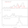 |
Fig. 2 Metallicity distributions of bulge and disk stars. In the top panel, the metallicity distributions of bulge dwarfs (black) and giants (red) are compared. |
Atomic parameters of the sulfur lines.
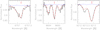 |
Fig. 3 Observed spectrum of the bulge star OGLE-2014-BLG-1418S (black) superimposed with the best fit (dashed red) synthetic spectrum. The contribution due to the terrestrial atmosphere is also shown (dotted blue). In the left, middle, and right panels, we report the S features (vertical red lines) of Mult. 8, 6, and 1, respectively. |
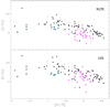 |
Fig. 4 [S/Fe]versus [Fe/H] diagram before (bottom panel) and after (top panel) NLTE corrections applied to the A(S) obtained in this work for bulge (black), thick-disk (cyan), and UVES POP thin-disk (magenta) stars. The bulge dwarfs and giants are shown as filled and open circles, respectively. |
5 Discussion
5.1 Sulfur behavior in the Galactic bulge
Several works confirm that S behaves like an α-element in the disk and halo of the MW (Francois 1987; Ryde & Lambert 2004; Caffau et al. 2007; Spite et al. 2011; Takeda et al. 2016). It is observed that from a constant value of [S/Fe] ~ +0.4 at low metallicity, [S/Fe] decreases with increasing [Fe/H] and it reaches [S/Fe] ~ 0 at solar metallicities (Nissen et al. 2007; Duffau et al. 2017). In contrast, other works found different S trends in the low-metallicity regime. The [S/Fe] value obtained by Israelian & Rebolo (2001) constantly increases as metallicity decreases, up to ~0.7–0.8 dex at − 2.3 < [Fe/H] < −1.9. Caffau et al. (2005) found a bimodal behavior of [S/Fe] (both stars with [S/Fe] ~ +0.4 and higher values) at low metallicity.
In Fig. 4, we compare the [S/Fe] versus [Fe/H] diagrams obtained before (bottom panel) and after (top panel) NLTE corrections for bulge stars (black). Both diagrams show that [S/Fe] decreases with the increase of [Fe/H] and that the bulge remains S-enhanced at solar metallicity. In the metal-poor regime, the small number of stars does not allow us to draw firm conclusions about the presence of a plateau. Considering the trend shown in Fig. 4, we can guess the presence of a plateau at the value [S/Fe]NLTE ~ +0.2 for [Fe/H] < −1. On this basis, we claim that S behaves like an α-element in the bulge. However, a larger number of metal-poor stars is required to robustly confirm or reject this claim.
Recently, Griffith et al. (2021) analyzed abundance ratio trends of sixteen species in the Galactic bulge and thick-disk red giant branch stars from the Apache Point Observatory Galactic Evolution Experiment (APOGEE, Blanton et al. 2017, Majewski et al. 2017) spectra. Among the different elements, the investigation of S in bulge stars was performed for the first time. They derived A(S) for ~11 000 targets in the metallicity range − 1.5 < [Fe/H] < 1 using S I lines at 15 478.5 and 16 576.6 Å, which are affected by small NLTE deviations (Jönsson et al. 2018, 2020; Korotin et al. 2020).
In Fig. 6, we compare our [S/Fe]NLTE (black) calculated considering features of Mults. 1, 6, and 8 (upper panel) and Mults. 6 and 8 only (bottom panel) with the median trend (open red squares) obtained by Griffith et al. (2021). In the bottom panel, our sample of bulge stars decreases to 37 due to the exclusion of Mult. 1, the strongest of the measured S lines and the most affected by NLTE deviations. However, we found similar S behavior in bulge stars at [Fe/H] > −0.2 when we consider Mult. 1, 6, and 8 (upper panel) corrected for NLTE effects and features less affected by NLTE deviation (bottom panel) to calculate S abundances.
Our results and those of Griffith et al. (2021) are similar in the metallicity range of − 1 < [Fe/H] < −0.1, while on average, our [S/Fe] ratios are higher in the range of [Fe/H] > 0.1 by about 0.04 ± 0.01 dex.
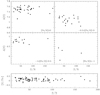 |
Fig. 5 A(S) versus S/N and [S/Fe] versus S/N diagrams. |
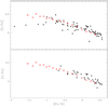 |
Fig. 6 [S/Fe] versus [Fe/H] diagram. The results obtained in this work for bulge stars (black) are compared with the mean trend (open red squares) of Griffith et al. (2021). [S/Fe]NLTE values of bulge stars were calculated considering features of Mults. 1, 6, and 8 and features of Mults. 6 and 8 in the upper and bottom panel, respectively. |
5.2 Comparison with sulfur abundances in the disk
In order to perform a homogeneous analysis of the bulge and the disk, a comparison sample of disk stars with stellar parameters derived in similar way is required. Indeed, differences in the choice made to estimate the stellar atmospheric parameters, particularly in the effective temperature scale, may lead to systematic differences in the derived abundances among different studies.
With the aim of overcoming this problem, we decided to derive the S abundance of a kinematically selected sample of thick- and thin-disk stars whose atmospheric parameters were determined consistently with our bulge stars.
We considered 21 thick-disk stars and 30 thin-disk stars that were previously analyzed by Bensby et al. (2014). The thick-disk stars are located between 14.8 and 109.9 pc from the Sun and within 2410 pc from the Galactic plane; whereas the thin-disk stars have heliocentric distance between 7.5 and 72 pc and a maximum distance from the Galactic plane of 680 pc.
The LTE (lower panel) and NLTE (upper panel) [S/Fe] values obtained from Mults. 1, 6, and 8 for the thick- (cyan) and thin- (magenta) disk stars are reported in Fig. 4. The comparison in Fig. 4 shows that the bulge is S-rich with respectto both the thick- and thin-disks.
Using the Gaia ESO Survey data (Gilmore et al. 2012); Duffau et al. (2017) measured S abundances of F and G-type stars in the solar neighborhood. Their dwarf stars sample is located within ≤ 1.5 kpc from the Sun at Galactic latitude ⟨|b|⟩≈ 30°, while giants cover a larger range in distance, 0 < D/kpc < 16, at ⟨|b|⟩≈ 9°. They foundthat their subsample of dwarfs is dominated by thick-disk stars at [Fe/H] < −0.5, while giant stars mainly belong to the thin-disk and dominate the sample at higher metallicities.
Recently, Perdigon et al. (2021) investigated the evolution of S in the Milky Way using FGK-type stars spectra provided by the Archéologie avec Matisse Basée sur les aRchives de l′ ESO (AMBRE) Project (de Laverny et al. 2013). Their sample of stars is located within 200 pc from the Sun and within a distance smaller than 400 pc from the Galactic plane. They identified two disk components characterized by different age, kinematics, and sulfur abundances. In order to distinguish the thin- and thick- disk, they defined a separation line in the [Fe/H] versus [S/Fe] plane. They associated the metal-poor, S-rich stars above the separation line with the thick- disk. The metal-rich, S-poor stars below the separation line were associated with the thin-disk. According to their work, the thick-disk component has low rotational velocities and is older than the thin-disk. The thick-disk is also S-rich with respect to the thin-disk in the metallicity range of − 1 ≤ [Fe/H] ≤−0.5. The thin-disk stars, instead, have rotational velocities close to the solar one and S abundances that slowly decrease from [Fe/H] ~−0.5 dex up to +0.5 dex.
Griffith et al. (2021) defined the Galactic thick-disk as stars with Galactocentric radius 5 kpc < RGC < 11 kpc and mid-plane distance |Z| < 2 kpc. Comparing the S evolution in the bulge and the thick-disk they found similar S median trends.
In Fig. 7 we compare our results with those mentioned above in the [S/Fe] versus [Fe/H] diagram. The bulge and the thick- and thin-disk stars analyzed in this work are reported as black, cyan, and magenta points, respectively. The green line in the upper panel is the mean trend of disk stars analyzed by Duffau et al. (2017) and is dominated by thick-disk stars at [Fe/H] < −0.5 and by thin-disk ones at higher metallicities. The separation line (gray) and the thick- and thin-disk areas (gray) defined by Perdigon et al. (2021) are shown in the bottom panel. In the upper panel, the bulge and the thick-disk stars studied by Griffith et al. (2021) are shown as red open squares and blue open triangle symbols.
In the metallicity range −1 < [Fe/H] < −0.5, the [S/Fe] values obtained in this work for thick-disk stars lie in the thick-disk area defined by Perdigon et al. (2021). On the other hand, we found that our thick-disk sample is 0.09 ± 0.05 dex and 0.14 ± 0.01 dex less S-enriched with respect to the thick-disk sample of Duffau et al. (2017) and Griffith et al. (2021), respectively.
Despite the low number of thick-disk stars at low and super-solar [Fe/H], we found that the bulge ischaracterized by a higher S content than the thick-disk in the metallicity range −1 < [Fe/H] < −0.5. This outcome is at odds with the result of Griffith et al. (2021), who found similar S trends for bulge (red open squares) and thick-disk (blue open triangles) stars.
Finally, the thin-disk stars are slightly less S-rich by 0.04 ± 0.02 dex than those studied by Duffau et al. (2017), while they are similar to the thin-disk population of Perdigon et al. (2021). We observe a substantial agreement between the thin- and thick-disk stars and the literature and we conclude that the bulge is S-enriched with respect to the thin- and thick-disk.
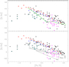 |
Fig. 7 [S/Fe] versus [Fe/H] diagrams. The [S/Fe]NLTE measured in this work for bulge and thick- and thin-dwarf stars are shown in black, cyan, and magenta points, respectively.The open red squares and open blue triangles are the median trends for bulge and thick-disk stars studied by Griffith et al. (2021). The mean trend obtained by Duffau et al. (2017) for Galactic-disk stars is reported as a green line. In the bottom panel are reported the thick- and thin-disk areas (gray) defined by Perdigon et al. (2021), and the line separating between them (gray continuous line). |
5.3 Comparison between α-elements in the bulge and the disk
From Fig. 7, it is clear that the trend in the [S/Fe] vs [Fe/H] plane is different for bulge and thin-disk stars. The situation is, on the other hand, less clear when considering the thick-disk. While we obtain different S content for bulge and thick-disk stars, Griffith et al. (2021) found a substantial agreement between their bulge and thick-disk stars. We note that the A(S) of the disk stars we analyzed are comparable with those of Duffau et al. (2017) and Perdigon et al. (2021).
The evidence of different [α/Fe] abundance trends between the bulge and the thin- and thick-disk was found by other studies, considering both dwarf (Bensby et al. 2017) and RGB (Rich & Origlia 2005; Zoccali et al. 2008) stars. According to Cunha & Smith (2006), the [O/Fe] and [Ti/Fe] trends of K and M RGB stars in the bulge fall above those of the thin- and the thick-disk. Fulbright et al. (2007) derived detailed abundances of O, Na, Mg, Al, Si, Ca, and Ti from high-resolution HIRES spectra of 27 RGB stars observed toward the Galactic bulge in the Baade’s window. They found that in the metallicity range of − 1.5 < [Fe/H] < 0.5, all the mean trends of α-elements in the bulge lie ~0.2 dex higher than that of the thin-disk. Johnson et al. (2014) analyzed the high resolution and high S/N FLAMES/GIRAFFE spectra of 156 RGB stars to estimate Mg, Si, Ca, and Ti abundances. Overall, they found that the bulge exhibits higher [α/Fe] ratios than the local thick-disk at [Fe/H] ≤−0.5. From APOGEE spectra of stars located in the Baade’s Window, Schultheis et al. (2017) obtained a median trend for bulge stars more enhanced than the thick-disk one in the [Mg/Fe] vs. [Fe/H] diagram.
However, there is no universal agreement in the literature that the [α/Fe] trends of bulge and thick-disk are different. According to Alves-Brito et al. (2010), the bulge and thick-disk follow the same [α/Fe] trend in the metallicity range − 1.5 < [Fe/H] < −0.3. This result is in good agreement with Hill et al. (2011), who found similar [Mg/Fe] trends in the bulge and the thick-disk at [Fe/H] < −0.4. On the other hand, the bulge shows higher [Mg/Fe] values than thick- and thin-disk ones at − 0.4 < [Fe/H] < −0.1, while similar [Mg/Fe] ratios between bulge and local thin-disk are found at [Fe/H] > −0.1 (Hill et al. 2011). Gonzalez et al. (2011, 2015) found that bulge and thick-disk have similar abundances of α-elements at low metallicity. Both are enhanced with respect to the thin-disk. At solar metallicities, the bulge presents [α/Fe] ratios similar to those of the thin-disk.
Thanks to the Gaia-ESO survey, Rojas-Arriagada et al. (2017) performed a homogeneous comparison between the bulge and the thin- and thick-disk sequences in the [Mg/Fe] versus [Fe/H] diagram. In this context, the bulge and thick-disk stars show similar [Mg/Fe] ratio levels over the whole metallicity range in common, while the bulge stars are shown to be Mg-enriched with respect to the thin-disk at [Fe/H] < 0.1 dex. Jönsson et al. (2017) performed a homogeneous analysis on α-elements in 46 and 291 K-type giants located in the bulge and local thick-disk, respectively, finding no different trends for these components of the MW.
Finally, we note that while for the sample of microlensed bulge stars, we find a mean [S/Fe] vs. [Fe/H] trend similar to Griffith et al. (2021), the same is not true for the other α-elements of the same stars. A significantly different trend can be appreciated at low metallicity between Griffith et al. (2021) and Bensby et al. 2017 (see O, Mg and Ca in Fig. 8). A detailed analysis of the differences between these two studies is beyond the scope of the present contribution. It is most likely that this is rooted in the different spectral ranges, the atomic and molecular data, as well as the different analysis methods employed. In Figs. 6–8, we show for comparison the mean trends of various [α/Fe] abundance ratios obtained from APOGEE data. We note, however, that the star-to-star scatter can be quite significant (see, for instance, Fig. 3 in Griffith et al. 2021 and Fig. 2 in Korotin et al. 2020).
In order to investigate the different α-elements behavior, wecreated [S/α] versus [Fe/H] diagrams. In Fig. 9, we compare the bulge (black), thick- (cyan) and thin- (magenta) disks trends. We found flat trends for the ratios of S over Mg, Si, and Ca for the bulge and disk samples, meaning that these elements are produced with no nuclosynthesis differences. On the other hand, more S is produced with respect to O as the metallicity increases. We should, however, remain aware that the O abundances of Bensby et al. (2014) were determined from the O I permitted triplet lines that are strongly affected both by departures from LTE and granulation effects (see e.g., Steffen et al. 2015; Amarsi et al. 2019, and references therein), the effects become larger at lower metallicity. Bensby et al. (2014) adopted the empirical correction of Bensby et al. (2004) to correct their LTE oxygen abundances, we should, however, be aware that the sample of stars that define this correction has [Fe/H] > −0.6 and thus the correction applied to stars beyond this metallicity is an extrapolation.
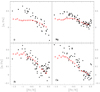 |
Fig. 8 [α/Fe] versus [Fe/H] diagrams. The O, Mg, Si, and Ca abundances measured by Bensby et al. (2017) for the bulge stars (black) analyzed in this work are compared to those of Griffith et al. (2021) (open red squares). |
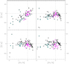 |
Fig. 9 [S/α] versus [Fe/H] diagrams of bulge (black) and thick- (cyan) and thin- (magenta) disk stars. The α-element abundances and metallicities come from the works of Bensby et al. (2014, 2017). |
6 Summary and conclusions
This work investigates the behavior of sulfur in the Galactic bulge. We used high-resolution, high S/N spectra of 74 dwarf and sub-giant stars, collected with UVES during microlensing events and investigated by Bensby et al. (2017). A reference sample of 21 and 30 F and G thick- and thin-disk stars located in the solar neighborhood was also analyzed. For all the samples, we used the atmospheric parameters estimated by Bensby et al. (2014, 2017, 2020) to measure A(S) from Mults. 1, 6, and 8.
Sulfur behaves similarly to the others α-elements in the bulge. While we can confirm the trend of [S/Fe] with [Fe/H] found by Griffith et al. (2021) in the bulge below metallicities [Fe/H] < −0.1, at higher metallicities, our [S/Fe] measurements are slightly, but systematically, higher.
In order to compare the bulge and disk stars whose atmospheric parameters were determined consistently, we measured A(S) of 21 and 30 thick- and thin-disk stars previously studied by Bensby et al. (2014). In the metallicity range of − 1< [Fe/H] < −0.5, our measurements in thick-disk stars are in agreement with Perdigon et al. (2021) and they agree within the errors with Duffau et al. (2017). On the other hand, our sample of thick-disk stars is S-poor with respect to Griffith et al. (2021). Overall, we found that the bulge has a higher S content than the thick-disk. This outcome stands in contradiction to the results of Griffith et al. (2021); however, it is in agreement with what has been found for other α-elements in other works (Rich & Origlia 2005; Cunha & Smith 2006; Fulbright et al. 2007; Zoccali et al. 2008; Johnson et al. 2014; Bensby et al. 2017; Schultheis et al. 2017).
The [S/Fe] values obtained for thin-disk stars are comparable with those reported by Duffau et al. (2017) and Perdigon et al. (2021). Our measurements imply that the bulge is S enriched with respect to the thin-disk at [Fe/H] > −0.4, which is in agreement with previous works (Fulbright et al. 2007; Johnson et al. 2014; Gonzalez et al. 2011, 2015; Schultheis et al. 2017; Rojas-Arriagada et al. 2017).
In conclusion, our sulfur abundances support a scenario in which the bulge and the disk have experienced different chemical enrichment and evolution processes. In particular, the S enhancement of bulge stars suggests that it was formed more rapidly than the disk.
Acknowledgements
The authors are grateful to the anonymous referee for providing helpful comments and suggestions, which have improved the content of this paper. Support for the author F.L. is provided by CONICYT-PFCHA/Doctorado Nacional año 2020-folio 21200677. E.C. and P.B. acknowledge support from the French National Research Agency (ANR) funded project “Pristine” (ANR-18-CE31-0017).
Appendix A Additional tables
Summary of bulge stars data. The target names, their coordinates and the S/N are listed in columns 2-5. The atmospheric parameters and radial velocities estimated by Bensby et al. 2017 follow in columns 7-11. The number of Sulfur line (N) used to estimate the NLTE Sulfur abundances obtained in this work are reported in the last two columns. The uncertainties on A(S) are the standard deviation.
Summary of thick-disk stars data. The target names and their coordinates are listed in columns 2-4. The atmospheric parameters estimated by Bensby et al. (2014) follow in columns 5-8. The number of Sulfur line (N) used to estimate the NLTE Sulfur abundances obtained in this work are reported in the last two columns. The uncertainties on A(S) are the standard deviation.
Summary of UVES POP stars data. The target names and their coordinates are listed in columns 2-4. The atmospheric parameters estimated by Bensby et al. (2014) follow in columns 5-8. The number of Sulfur line (N) used to estimate the NLTE Sulfur abundances obtained in this work are reported in the last two columns. The uncertainties on A(S) are the standard deviation.
References
- Alves-Brito, A., Meléndez, J., Asplund, M., Ramírez, I., & Yong, D. 2010, A&A, 513, A35 [NASA ADS] [CrossRef] [EDP Sciences] [Google Scholar]
- Amarsi, A. M., Nissen, P. E., & Skúladóttir, Á. 2019, A&A, 630, A104 [NASA ADS] [CrossRef] [EDP Sciences] [Google Scholar]
- Athanassoula, E. 2005, MNRAS, 358, 1477 [NASA ADS] [CrossRef] [Google Scholar]
- Bagnulo, S., Jehin, E., Ledoux, C., et al. 2003, The Messenger, 114, 10 [Google Scholar]
- Bensby, T., Feltzing, S., & Lundström, I. 2003, A&A, 410, 527 [CrossRef] [EDP Sciences] [Google Scholar]
- Bensby, T., Feltzing, S., & Lundström, I. 2004, A&A, 415, 155 [NASA ADS] [CrossRef] [EDP Sciences] [Google Scholar]
- Bensby, T., Johnson, J. A., Cohen, J., et al. 2009, A&A, 499, 737 [NASA ADS] [CrossRef] [EDP Sciences] [Google Scholar]
- Bensby, T., Asplund, M., Johnson, J. A., et al. 2010a, A&A, 521, L57 [NASA ADS] [CrossRef] [EDP Sciences] [Google Scholar]
- Bensby, T., Feltzing, S., Johnson, J. A., et al. 2010b, A&A, 512, A41 [NASA ADS] [CrossRef] [EDP Sciences] [Google Scholar]
- Bensby, T., Adén, D., Meléndez, J., et al. 2011, A&A, 533, A134 [NASA ADS] [CrossRef] [EDP Sciences] [Google Scholar]
- Bensby, T., Yee, J. C., Feltzing, S., et al. 2013, A&A, 549, A147 [NASA ADS] [CrossRef] [EDP Sciences] [Google Scholar]
- Bensby, T., Feltzing, S., & Oey, M. S. 2014, A&A, 562, A71 [NASA ADS] [CrossRef] [EDP Sciences] [Google Scholar]
- Bensby, T., Feltzing, S., Gould, A., et al. 2017, A&A, 605, A89 [NASA ADS] [CrossRef] [EDP Sciences] [Google Scholar]
- Bensby, T., Feltzing, S., Yee, J. C., et al. 2020, A&A, 634, A130 [NASA ADS] [CrossRef] [EDP Sciences] [Google Scholar]
- Blanton, M. R., Bershady, M. A., Abolfathi, B., et al. 2017, AJ, 154, 28 [Google Scholar]
- Blumenthal, G. R., Faber, S. M., Primack, J. R., & Rees, M. J. 1984, Nature, 311, 517 [Google Scholar]
- Bournaud, F., Elmegreen, B. G., & Martig, M. 2009, ApJ, 707, L1 [Google Scholar]
- Caffau, E., Bonifacio, P., Faraggiana, R., et al. 2005, A&A, 441, 533 [NASA ADS] [CrossRef] [EDP Sciences] [Google Scholar]
- Caffau, E., Faraggiana, R., Bonifacio, P., Ludwig, H. G., & Steffen, M. 2007, A&A, 470, 699 [NASA ADS] [CrossRef] [EDP Sciences] [Google Scholar]
- Caffau, E., Ludwig, H. G., Steffen, M., Freytag, B., & Bonifacio, P. 2011, Sol. Phys., 268, 255 [Google Scholar]
- Castelli, F., & Kurucz, R. L. 2003, IAU Symp., 210, A20 [Google Scholar]
- Clarkson, W., Sahu, K., Anderson, J., et al. 2008, ApJ, 684, 1110 [NASA ADS] [CrossRef] [Google Scholar]
- Cunha, K., & Smith, V. V. 2006, ApJ, 651, 491 [NASA ADS] [CrossRef] [Google Scholar]
- de Laverny, P., Recio-Blanco, A., Worley, C. C., et al. 2013, The Messenger, 153, 18 [NASA ADS] [Google Scholar]
- Dekker, H., D’Odorico, S., Kaufer, A., Delabre, B., & Kotzlowski, H. 2000, SPIE Conf. Ser., 4008, 534 [Google Scholar]
- Dotter, A., Chaboyer, B., Jevremović, D., et al. 2008, ApJS, 178, 89 [Google Scholar]
- Duffau, S., Caffau, E., Sbordone, L., et al. 2017, A&A, 604, A128 [NASA ADS] [CrossRef] [EDP Sciences] [Google Scholar]
- Eggen, O. J., Lynden-Bell, D., & Sandage, A. R. 1962, ApJ, 136, 748 [NASA ADS] [CrossRef] [Google Scholar]
- Epstein, C. R., Johnson, J. A., Dong, S., et al. 2010, ApJ, 709, 447 [NASA ADS] [CrossRef] [Google Scholar]
- Francois, P. 1987, A&A, 176, 294 [NASA ADS] [Google Scholar]
- Fulbright, J. P., McWilliam, A., & Rich, R. M. 2007, ApJ, 661, 1152 [NASA ADS] [CrossRef] [Google Scholar]
- Gennaro, M., Brown, T., Anderson, J., et al. 2015, ASP Conf. Ser., 491, 182 [NASA ADS] [Google Scholar]
- Genzel, R., Burkert, A., Bouché, N., et al. 2008, ApJ, 687, 59 [Google Scholar]
- Gilmore, G., Randich, S., Asplund, M., et al. 2012, The Messenger, 147, 25 [NASA ADS] [Google Scholar]
- Gonzalez, O. A., Rejkuba, M., Zoccali, M., et al. 2011, A&A, 530, A54 [NASA ADS] [CrossRef] [EDP Sciences] [Google Scholar]
- Gonzalez, O. A., Zoccali, M., Vasquez, S., et al. 2015, A&A, 584, A46 [NASA ADS] [CrossRef] [EDP Sciences] [Google Scholar]
- Griffith, E., Weinberg, D. H., Johnson, J. A., et al. 2021, ApJ, 909, 77 [NASA ADS] [CrossRef] [Google Scholar]
- Hill, V., Lecureur, A., Gómez, A., et al. 2011, A&A, 534, A80 [NASA ADS] [CrossRef] [EDP Sciences] [Google Scholar]
- Israelian, G., & Rebolo, R. 2001, ApJ, 557, L43 [Google Scholar]
- Johnson, C. I., Rich, R. M., Kobayashi, C., Kunder, A., & Koch, A. 2014, AJ, 148, 67 [Google Scholar]
- Jönsson, H., Ryde, N., Schultheis, M., & Zoccali, M. 2017, A&A, 598, A101 [NASA ADS] [CrossRef] [EDP Sciences] [Google Scholar]
- Jönsson, H., Allende Prieto, C., Holtzman, J. A., et al. 2018, AJ, 156, 126 [Google Scholar]
- Jönsson, H., Holtzman, J. A., Allende Prieto, C., et al. 2020, AJ, 160, 120 [Google Scholar]
- Kobayashi, C., Karakas, A. I., & Lugaro, M. 2020, ApJ, 900, 179 [Google Scholar]
- Kormendy, J., & Kennicutt, Robert C., J. 2004, ARA&A, 42, 603 [NASA ADS] [CrossRef] [Google Scholar]
- Korotin, S. A., Andrievsky, S. M., Caffau, E., Bonifacio, P., & Oliva, E. 2020, MNRAS, 496, 2462 [NASA ADS] [CrossRef] [Google Scholar]
- Kurucz, R. 1993a, ATLAS9 Stellar Atmosphere Programs and 2 km/s grid. Kurucz CD-ROM No. 13. Cambridge, 13 [Google Scholar]
- Kurucz, R. L. 1993b, SYNTHE Spectrum Synthesis Programs and Line Data (Cambridge, Mass.: Smithsonian Astrophysical Observatory) [Google Scholar]
- Kurucz, R. L. 2005, Mem. Soc. Astron. It. Suppl., 8, 14 [Google Scholar]
- Limongi, M., & Chieffi, A. 2003, ApJ, 592, 404 [CrossRef] [Google Scholar]
- Majewski, S. R., Schiavon, R. P., Frinchaboy, P. M., et al. 2017, AJ, 154, 94 [NASA ADS] [CrossRef] [Google Scholar]
- Matteucci, F., & Brocato, E. 1990, ApJ, 365, 539 [CrossRef] [Google Scholar]
- McWilliam, A., & Rich, R. M. 1994, ApJS, 91, 749 [NASA ADS] [CrossRef] [Google Scholar]
- Meléndez, J., Asplund, M., Alves-Brito, A., et al. 2008, A&A, 484, L21 [NASA ADS] [CrossRef] [EDP Sciences] [Google Scholar]
- Mucciarelli, A., Pancino, E., Lovisi, L., Ferraro, F. R., & Lapenna, E. 2013, Astrophysics Source Code Library [record ascl:1302.011] [Google Scholar]
- Ness, M., & Freeman, K. 2012, EPJ Web Conf., 19, 06003 [NASA ADS] [CrossRef] [EDP Sciences] [Google Scholar]
- Nissen, P. E., Akerman, C., Asplund, M., et al. 2007, A&A, 469, 319 [NASA ADS] [CrossRef] [EDP Sciences] [Google Scholar]
- Perdigon, J., de Laverny, P., Recio-Blanco, A., et al. 2021, A&A 647, A162 [NASA ADS] [CrossRef] [EDP Sciences] [Google Scholar]
- Perryman, M. A. C., Lindegren, L., Kovalevsky, J., et al. 1997, A&A, 323, L49 [Google Scholar]
- Rahimi, A., Kawata, D., Brook, C. B., & Gibson, B. K. 2010, MNRAS, 401, 1826 [NASA ADS] [CrossRef] [Google Scholar]
- Renzini, A., Gennaro, M., Zoccali, M., et al. 2018, ApJ, 863, 16 [NASA ADS] [CrossRef] [Google Scholar]
- Rich, R. M., & Origlia, L. 2005, ApJ, 634, 1293 [NASA ADS] [CrossRef] [Google Scholar]
- Rich, R. M., Reitzel, D. B., Howard, C. D., & Zhao, H. 2007, ApJ, 658, L29 [NASA ADS] [CrossRef] [Google Scholar]
- Robertson, B., Bullock, J. S., Cox, T. J., et al. 2006, ApJ, 645, 986 [NASA ADS] [CrossRef] [Google Scholar]
- Rojas-Arriagada, A., Recio-Blanco, A., Hill, V., et al. 2014, A&A, 569, A103 [NASA ADS] [CrossRef] [EDP Sciences] [Google Scholar]
- Rojas-Arriagada, A., Recio-Blanco, A., de Laverny, P., et al. 2017, A&A, 601, A140 [NASA ADS] [CrossRef] [EDP Sciences] [Google Scholar]
- Ryde, N., & Lambert, D. L. 2004, A&A, 415, 559 [EDP Sciences] [Google Scholar]
- Ryde, N., Edvardsson, B., Gustafsson, B., et al. 2009, A&A, 496, 701 [NASA ADS] [CrossRef] [EDP Sciences] [Google Scholar]
- Schultheis, M., Rojas-Arriagada, A., García Pérez, A. E., et al. 2017, A&A, 600, A14 [NASA ADS] [CrossRef] [EDP Sciences] [Google Scholar]
- Spite, M., Caffau, E., Andrievsky, S. M., et al. 2011, A&A, 528, A9 [NASA ADS] [CrossRef] [EDP Sciences] [Google Scholar]
- Steffen, M., Prakapavičius, D., Caffau, E., et al. 2015, A&A, 583, A57 [NASA ADS] [CrossRef] [EDP Sciences] [Google Scholar]
- Takeda, Y., Hashimoto, O., Taguchi, H., et al. 2005, PASJ, 57, 751 [NASA ADS] [Google Scholar]
- Takeda, Y., Omiya, M., Harakawa, H., & Sato, B. 2016, PASJ, 68, 81 [Google Scholar]
- Zoccali, M., Lecureur, A., Hill, V., et al. 2008, Mem. Soc. Astron. It., 79, 503 [NASA ADS] [Google Scholar]
- Zoccali, M., Vasquez, S., Gonzalez, O. A., et al. 2017, A&A, 599, A12 [NASA ADS] [CrossRef] [EDP Sciences] [Google Scholar]
IRAF is distributed by the National Optical Astronomy Observatory, which is operated by the Association of Universities for Research in Astronomy (AURA) under a cooperative agreement with the National Science Foundation.
All Tables
Summary of bulge stars data. The target names, their coordinates and the S/N are listed in columns 2-5. The atmospheric parameters and radial velocities estimated by Bensby et al. 2017 follow in columns 7-11. The number of Sulfur line (N) used to estimate the NLTE Sulfur abundances obtained in this work are reported in the last two columns. The uncertainties on A(S) are the standard deviation.
Summary of thick-disk stars data. The target names and their coordinates are listed in columns 2-4. The atmospheric parameters estimated by Bensby et al. (2014) follow in columns 5-8. The number of Sulfur line (N) used to estimate the NLTE Sulfur abundances obtained in this work are reported in the last two columns. The uncertainties on A(S) are the standard deviation.
Summary of UVES POP stars data. The target names and their coordinates are listed in columns 2-4. The atmospheric parameters estimated by Bensby et al. (2014) follow in columns 5-8. The number of Sulfur line (N) used to estimate the NLTE Sulfur abundances obtained in this work are reported in the last two columns. The uncertainties on A(S) are the standard deviation.
All Figures
|
Fig. 1 log(g) versus log(Teff) diagrams of the stellar sample considered in this work. The bulge and the thick- and thin-disk stars are shown in black, cyan, and magenta respectively. The black filled circle and open circles are bulge dwarfs and giants. In each panel, we show the metallicities and the ages adopted to obtain isochrones from the Dartmouth Stellar Evolution Database (Dotter et al. 2008). |
| In the text | |
|
Fig. 2 Metallicity distributions of bulge and disk stars. In the top panel, the metallicity distributions of bulge dwarfs (black) and giants (red) are compared. |
| In the text | |
|
Fig. 3 Observed spectrum of the bulge star OGLE-2014-BLG-1418S (black) superimposed with the best fit (dashed red) synthetic spectrum. The contribution due to the terrestrial atmosphere is also shown (dotted blue). In the left, middle, and right panels, we report the S features (vertical red lines) of Mult. 8, 6, and 1, respectively. |
| In the text | |
|
Fig. 4 [S/Fe]versus [Fe/H] diagram before (bottom panel) and after (top panel) NLTE corrections applied to the A(S) obtained in this work for bulge (black), thick-disk (cyan), and UVES POP thin-disk (magenta) stars. The bulge dwarfs and giants are shown as filled and open circles, respectively. |
| In the text | |
|
Fig. 5 A(S) versus S/N and [S/Fe] versus S/N diagrams. |
| In the text | |
|
Fig. 6 [S/Fe] versus [Fe/H] diagram. The results obtained in this work for bulge stars (black) are compared with the mean trend (open red squares) of Griffith et al. (2021). [S/Fe]NLTE values of bulge stars were calculated considering features of Mults. 1, 6, and 8 and features of Mults. 6 and 8 in the upper and bottom panel, respectively. |
| In the text | |
|
Fig. 7 [S/Fe] versus [Fe/H] diagrams. The [S/Fe]NLTE measured in this work for bulge and thick- and thin-dwarf stars are shown in black, cyan, and magenta points, respectively.The open red squares and open blue triangles are the median trends for bulge and thick-disk stars studied by Griffith et al. (2021). The mean trend obtained by Duffau et al. (2017) for Galactic-disk stars is reported as a green line. In the bottom panel are reported the thick- and thin-disk areas (gray) defined by Perdigon et al. (2021), and the line separating between them (gray continuous line). |
| In the text | |
|
Fig. 8 [α/Fe] versus [Fe/H] diagrams. The O, Mg, Si, and Ca abundances measured by Bensby et al. (2017) for the bulge stars (black) analyzed in this work are compared to those of Griffith et al. (2021) (open red squares). |
| In the text | |
|
Fig. 9 [S/α] versus [Fe/H] diagrams of bulge (black) and thick- (cyan) and thin- (magenta) disk stars. The α-element abundances and metallicities come from the works of Bensby et al. (2014, 2017). |
| In the text | |
Current usage metrics show cumulative count of Article Views (full-text article views including HTML views, PDF and ePub downloads, according to the available data) and Abstracts Views on Vision4Press platform.
Data correspond to usage on the plateform after 2015. The current usage metrics is available 48-96 hours after online publication and is updated daily on week days.
Initial download of the metrics may take a while.