| Issue |
A&A
Volume 655, November 2021
|
|
|---|---|---|
| Article Number | A55 | |
| Number of page(s) | 16 | |
| Section | Galactic structure, stellar clusters and populations | |
| DOI | https://doi.org/10.1051/0004-6361/202140984 | |
| Published online | 19 November 2021 | |
Precessing ellipses as the building blocks of spiral arms
1
Research center for Astronomy and Applied Mathematics, Academy of Athens, Soranou Efessiou 4, 115 27 Athens, Greece
e-mail: This email address is being protected from spambots. You need JavaScript enabled to view it.
; This email address is being protected from spambots. You need JavaScript enabled to view it.
2
Department of Physics, Section of Astrophysics, Astronomy and Mechanics, University of Athens, Panepistimiopolis, 15784 Athens, Greece
e-mail: This email address is being protected from spambots. You need JavaScript enabled to view it.
3
Department of Mathematics, Tullio Levi-Civita, University of Padua, Via Trieste, 63, 35121 Padova, Italy
Received:
2
April
2021
Accepted:
9
August
2021
Abstract
Stable periodic orbits in spiral galactic models that form families of precessing ellipses can create spiral density waves similar to those that are observed in real grand-design galaxies. We study the range in parameter space for which the amplitude of the spiral perturbation, the pattern speed, and the pitch angle collaborate so as to lead to the creation of density waves that are supported by precessing ellipses and their surrounding matter in ordered motion. Quantitative estimates lead to a correlation between the pitch angle and the amplitude of the spiral perturbation and also between the pitch angle and the pattern speed of the spiral arms. These correlations can be regarded as an orbital analog of a nonlinear dispersion relation in density wave theory.
Key words: galaxies: kinematics and dynamics
© ESO 2021
1. Introduction
The ubiquity of grand-design bisymmetric spiral arms that are observed in galactic disks in the K band indicates that the paradigm of the “density wave” remains a valid dynamical model with which the spiral structure of many disk galaxies can be described. While the scenario of quasi-stationary spiral density waves has been strongly criticized (see Toomre 1977; Athanassoula 1984; Binney & Tremaine 2008; Sellwood & Carlberg 1984; Sellwood 2010; Dobbs & Baba 2014 for reviews), the existence of mechanisms regulating the growth rate of spiral density waves, and hence ensuring their longevity for several pattern periods, remains largely an open question (Bertin 1980; Donner & Thomasson 1994, see Bertin & Lin 1996; Contopoulos 2002 for reviews). The density wave theory fits the description of spiral arms betten when the spiral amplitude does not exceed a value of 10%−20% over a timescale of a few (≈5) pattern rotations. In this regime, nonlinear corrections (Contopoulos 1970; Vandervoort 1971; Norman 1978) to the linear Lindblad-Lin-Shu theory are required (Lindblad 1940, 1961; Lin & Shu 1964, 1966).
The basic formulation of density wave theory (see Binney & Tremaine 2008) deals with spiral wave perturbations in an axisymmetric disk that is regarded in the framework of either the Boltzmann equation for collisionless matter or the hydrodynamical equations for gas. On the other hand, Lindblad (1955) pioneered the orbital description of spiral density waves. In this description, the central objective is to identify the main families of stellar orbits that support the spirals, and also to show how these orbits can collaborate to match the imposed with the response model of spiral arms (see Contopoulos 1971; Berman & Mark 1977; Monet & Vandervoort 1978; Contopoulos & Grosbøl 1986; Patsis et al. 1991). In the orbital description of spiral density waves, a key element are approximately elliptical stable periodic orbits whose orientation changes with the distance from the center (parameterized by the Jacobi energy) so as to produce a response density that closely follows the minima of the imposed spiral potential. The importance of these periodic orbits as the building blocks of spiral arms was first stressed by Lindblad (1956, 1957, 1958, 1960, 1961), who called them “dispersion orbits”. Contopoulos (1970, 1975) developed the theory of resonant periodic orbits near the inner Linblad resonance, providing the main formulas that allow predicting the number and stability of the periodic orbits as a function of the Jacobi energy. The resonant theory of Contopoulos, based on epicyclic action-angle variables, also allows predicting the structure of the phase space around the periodic orbits, yielding the corresponding invariant curves as the level curves of a resonant “third integral” (see Contopoulos 2002 for a review). The predictions of this theory were confirmed by Vandervoort (1973, 1975; see also Vandervoort 1975 and Monet & Vandervoort 1978), Mertzanides (1976) and Berry & Smet (1979). These studies provided figures of the corresponding phase portraits around the elliptical closed orbits computed analytically (by the third integral) or numerically in simple models of galactic potentials with a spiral perturbation. On the other hand, Kalnajs (1973) popularized the orbital version of the density wave theory by providing a schematic figure of the emergence of spiral arms due to the change in orientation of the axes of the elliptical orbits (“precessing ellipses”), a figure that was later reproduced in many reviews and books on the subject. Kalnajs (1973) also computed an approximative formula for the response spiral potential due to the precessing ellipses, which holds beyond the Wentzel-Kramers-Brillouin (WKB) limit of tightly wound spirals. The overall limit of the applicability of the precessing ellipses was considered by Contopoulos (1985). The change in orientation of the elliptical orbits with the energy is explained by resonant perturbation theory (Contopoulos 1975, 2002; Monet & Vandervoort 1978, see a tutorial presentation in Efthymiopoulos 2010). Numerical examples of spirals supported by precessing ellipses have been computed in models of spiral galaxies (Contopoulos & Grosbøl 1986; Patsis et al. 1991; Patsis & Grosbøl 1996; Pichardo et al. 2003; Efthymiopoulos 2010; Tsigaridi & Patsis 2013; Pérez-Villegas et al. 2015; Chaves-Velasquez et al. 2019).
An important outcome of linear density wave theory, which is valid for small amplitudes of the spiral perturbation, is the dispersion relation (see Binney & Tremaine 2008, p. 493), which relates the frequency (pattern speed Ωsp of the spiral arms) with the radial wavenumber k. For tightly wound m = 2 logarithmic spirals, the radial wavenumber k and the pitch angle α are related by α = cot−1(k r/2). In order to understand the relevance of the dispersion relation to our results below, we point out that in a given (and fixed) axisymmetric model, the dispersion relation depends on the quantities κ(r) (epicyclic frequency), Ω(r) (angular velocity of the circular orbit of radius r), and Σ0(r) (axisymmetric disk, as well as on the velocity dispersion σ(r) at radius r. All these quantities are completely specified by the model that is used to represent the axisymmetric component of the disk, that is, by the potential Vax(r) and by the form Q(r) of the profile of Toomre’s Q-parameter as a function of the distance from the center (see Eq. (15) below). Thus, after an axisymmetric model is fixed, the dispersion relation should be regarded as a relation allowing us to specify the form of the function k(r; Ωsp), where k = dϕm(r)/dr and ϕm is the phase (position of maxima) of the m-fold spiral mode. Hence, solving the differential equation (for m = 2 spiral arms) dϕ2(r)/dr = k(r; Ωsp), we obtain the form of the phase ϕ2(r; Ωsp) corresponding to the maxima of the spiral arms. This implies that within a fixed axisymmetric background (potential + velocity dispersion), the linear dispersion relation establishes a correlation between the form of the spiral arms (given by the function ϕ2) and the value of the spiral pattern speed Ωsp. It is important to emphasize that in the linear regime, this relation is independent of the amplitude of the spiral perturbation, which is simplified altogether from the equations of the linear theory.
However, in nonlinear wave theory, the amplitude of the spiral perturbation A(r) also has to be taken into account (see Contopoulos 1975, 1980; Norman 1978). This leads to a form of the dispersion relation that correlates all three basic parameters of the spirals, namely, the amplitude A(r), the pitch angle a, and the pattern speed Ωsp.
Regarded from the orbital point of view, two important nonlinear effects are introduced when the amplitude of the spirals becomes large:
-
(i)
the ‘precessing ellipses’ (closed orbits of the x1 family) become largely distorted with respect to the elliptical shape, and
-
(ii)
chaos is introduced in the system, leading to the lack of a sufficient number of regular orbits to support the spiral arms.
While these two phenomena have been stressed in previous studies (Contopoulos 1985; Contopoulos & Grosbøl 1986; Patsis et al. 1991, see also Quillen & Minchev 2005), a systematic study yielding the permissible space in all three parameters (A, a, and Ωsp) within which the precessing ellipses can support spiral arms is still lacking, in the literature. This constitutes the primary motivation for our present study. In particular, we first work with a simple model in which the axisymmetric components (disk and halo) have parameters with values that are pertinent to a Milky Way model. A bulge is added to properly secure good kinematic properties of the orbits at all distances across the disk. We then superpose a m = 2 logarithmic spiral term to the axisymmetric potential with a varying amplitude, pitch angle, and pattern speed, and study the corresponding phase-space structure in the region from the inner Lindblad resonance (ILR) to corotation. Our study focuses on the structure of the characteristic curve and the stability of the x1 family of periodic orbits, along with the extent of the domain of regular orbits around the x1 family. We also discuss the role of other families generated near the ILR (in particular, the x2 family), as well as the range in the parameter values in which the change in pericenter over galactocentric distance r is such as to support a spiral response similar to the one imposed by the model.
Second, stemming from the basic steps of resonant perturbation theory at the ILR, a byproduct of our analysis is to show the convenience of a particular set of variables in illustrating all phenomena relevant to the phase-space structure in the region from the IRL and up to the 4:1 resonance. Thus, we depict all numerical phase portraits (Poincaré surfaces of section) using the epicyclic set of canonical variables (ξ, pξ), where ξ = r − rc,  , and rc is the radius of the circular orbit of a fixed Jacobi energy h in the flow under the axisymmetric potential alone. Furthermore, we depict the characteristic curves of closed orbits (x1, x2, etc.) showing the quantity
 (1)
(1)
against rc, where (ξ0, pξ, 0) is the fixed point at which a closed orbit intersects a surface of section defined by a fixed azimuth. This choice of variables (instead of the customary choice, i.e., ξ0 as a function of h) is motivated by the fact that according to resonant perturbation theory, the relevant quantity characterizing the precessing ellipses is the amplitude of the epicyclic oscillation for a particular closed orbit, quantified by S(rc), as a function of the average distance of the orbit from the center of the disk. We find that spiral arms are in general supported by orbits for which S(rc) is a decaying function of rc (see Sect. 4).
Third, we identify the appearance of chaos as the main dynamical phenomenon defining the boundary of the domain in parameter space (A, a, and Ωsp), outside which spiral arms supported by precessing ellipses cannot exist. A good criterion for determining this boundary is obtained by computing the threshold in (A, a, and Ωsp) beyond which the x1 family itself becomes unstable at distances already close to the ILR. This threshold practically marks the nearly complete disappearance of ordered orbits in phase space. Detailed numerical evidence of these phenomena is given at the end of Sect. 4, leading to conclusions that approximately agree with the predictions of density wave theory, and probably also with observations (see the discussion at the end of Sect. 4). In particular, this orbital analysis supports the prediction that larger spiral amplitudes A as well as slower rotation (smaller Ωsp) are consistent with more open spirals (higher values of the pitch angle).
The paper is structured as follows. Section 2 presents our model. Section 3 discusses the construction of spiral density waves using closed orbits. In Sect. 4, an explanation is given of how periodic orbits are determined and how the phase space is constructed. Moreover, the main results of the paper are presented in this section, where we study the role of the amplitude of the spiral perturbation, the pattern speed of the spirals, and the pitch angle in creating realistic spiral density waves. Finally, we summarize our conclusions in Sect. 5.
2. Model
We considered a model of a spiral galaxy that contains a combination of an axisymmetric and a spiral potential,
 (2)
(2)
The axisymmetric potential Vax is composed of a disk, a bulge, and a halo,
 (3)
(3)
For the disk potential Vd, we used a Miyamoto-Nagai model (Miyamoto & Nagai 1975) given by the relation
 (4)
(4)
where Md = 8.56 × 10¹⁰ M⊙ is the total mass of the disk, ad = 5.3 kpc and bd = 0.25 kpc. In order to have a 2D disk model, we took z = 0 and  . For the bulge, we used a Plummer potential Vb given by the relation
 (5)
(5)
where Mb = 5 × 10¹⁰ M⊙ is the total mass of the bulge,  and b = 1.5 kpc.
The halo potential was a γ-model (Dehnen 1993) with parameters as in Pettitt et al. (2014),
![Mathematical equation: $$ \begin{aligned} V_{\rm {h}}=\frac{-GM_{\rm {h(r)}}}{r}-\frac{-GM_{\rm {h,0}}}{\gamma r_{\rm {h}}} \left[-\frac{\gamma }{1+(r/r_{\rm {h}})^\gamma }+\ln (1+\frac{r}{r_{\rm {h}}})^\gamma \right]_r^{r_{\rm h,max}}, \end{aligned} $$](/articles/aa/full_html/2021/11/aa40984-21/aa40984-21-eq9.gif) (6)
(6)
where rh, max = 100 kpc, γ = 1.02, and Mh, 0 = 10.7 × 10¹⁰ M⊙, and Mh(r) was given by the function:
 (7)
(7)
The spiral potential is given by the value Vsp for z = 0 of the 3D logarithmic spiral model Vsp(r, ϕ, z) introduced by Cox & Gómez (2002) (see formula (19) in Efthymiopoulos et al. 2020). We have on the disk plane
![Mathematical equation: $$ \begin{aligned} V_{\rm {sp}}\!=\! 4 \pi G h_{\rm {z}} \rho _{0} G(r)\exp \! \left(- \left(\frac{r- r_{\rm {0}}}{ R_{\rm {s}}} \right) \right)\! {\frac{C}{K B}}\! \cos \! \left[ 2 \!\left(\varphi \!-\!\frac{\ln (r/ r_{0} )}{\tan (\alpha )} \right) \right] , \end{aligned} $$](/articles/aa/full_html/2021/11/aa40984-21/aa40984-21-eq11.gif) (8)
(8)
where
 (9)
(9)
and C = 8/(3π), hz = 0.18 kpc, r0 = 8 kpc, Rs = 7 kpc, and a = −13° was the pitch angle of the spiral arms. The function G(r) plays the role of a smooth envelope determining the radius beyond which the spiral arms are important. We adopted the form G(r) = b − carctan((Rs0 − r)), with Rs0 = 6 kpc, b = 0.474, and c = 0.335. The spiral density was ρ0 = 5 × 10⁷, 15 × 107, or 30 × 107 M⊙ kpc−3 in the three different models under study, respectively. These three values of the density were chosen so as to yield spiral F-strength values consistent with those reported in the literature for a weak intermediate and strong spiral, respectively (see, e.g., Block et al. 2004).
The F-strength (Buta et al. 2009) can be defined as either the ratio of the maximum tangential force of the spiral perturbation over the radial force of the axisymmetric background,
 (10)
(10)
or the ratio of the maximum total force of the spiral perturbation over the radial force of the axisymmetric background, given by the relation
 (11)
(11)
Figure 1 shows Fall as a function of the radius derived from Eq. (11) for three different values of the density ρ0 of Eq. (8), namely ρ0 = 5,15,30(× 107) M⊙ kpc−3. The maximum values of the spiral F-strength were 5%, 15%, and 30%, respectively. In the intermediate model, the F-strength varies between 5% and 15% in the region 5 kpc ≤r ≤ 15 kpc. We note that the observed amplitudes (in F−strength) of the spirals in grand-design galaxies with respect to the axisymmetric background have typical values between 5% and 10% (Patsis et al. 1991; Grosbøl et al. 2004).
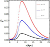 |
Fig. 1. Total force perturbation Fall for different amplitudes of the spiral potential as a function of the radius. |
Figure 2a shows the surface density profile corresponding to the sum of the disk and bulge component, while Fig. 2b shows the rotation curve produced by the potential Vax by the equation:  .
.
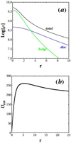 |
Fig. 2. (a) Surface density profile of the axisymmetric part of the model. The green curve represents the bulge, the blue curve represents the disk, and the black curve is the total profile. (b) Rotation velocity curve produced by the axisymmetric potential Vax. |
Figure 3 shows an isodensity color map of the projected surface density  in the disk plane, where the density ρ is computed from Poisson’s equation ∇2V = 4πGρ for the 3D potential model V(r, ϕ, z) = Vd(r)+Vb(r)+Vsp(r, ϕ, z). It is easy to check that the function ρ(r) is positive everywhere with this choice of potential model (see also Pettitt et al. 2014 and references within and Efthymiopoulos et al. 2020). The maxima of the density are plotted in red. Superimposed are the spiral arms (black curves) derived from the minima of the spiral potential of Eq. (8), which almost completely coincide with the maxima of the projected density of the galactic model. We note that the phase differences between the minima of the potential and the maxima of the spiral density have been suggested to be important close to and outside the corotation region (for a review, see Zhang 2018). However, the spirals considered in our work end at the 4:1 resonance (see below), which is reached well before the corotation region. In the following plots, we therefore use the minima of the potential as indicating the shapes of the imposed spirals for simplicity.
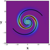 |
Fig. 3. Isodensities of the projected surface density of the 3D galactic model (see text). Superimposed are the spiral arms derived from the minima of the spiral potential of Eq. (8). |
When a fixed pattern speed Ωsp of the spirals is assumed, the Hamiltonian of stellar orbits in the disk plane in the rotating frame of reference, in polar coordinates, can be expressed as
 (12)
(12)
where pr and pφ are the values of the radial velocity and angular momentum per unit mass in the rest frame.
The angular velocity Ω(rc) of a star that moves in a circular orbit of radius rc under the action of the axisymmetric potential alone is given by the relation
 (13)
(13)
The epicyclic frequency κ(rc) at r = rc is given by
 (14)
(14)
Figure 4 shows the function Ω(r), as well as the combinations Ω − κ/2, Ω + κ/2 and Ω − κ/4. The section of Ω(r) with the pattern speed Ωsp defines the radius of the corotation, while the section of the frequency Ω − κ/2 (or Ω + κ/2) with the pattern speed Ωsp defines the radius of the ILR (or the outer Lindblad resonance, OLR). Depending on the model, we may have one or two ILRs. Our model (Fig. 4) has two ILRs, the first and the second ILR, as long as Ωsp < 20 km s−1 kpc−1. Finally, the section of the frequency Ω − κ/4 with the pattern speed Ωsp defines the radius of the 4:1 resonance. We studied the orbits for three different values of the pattern speed of the spiral potential Ωsp = 10, 15, and 20 km s−1 kpc−1 (see Sect. 4.2.2).
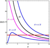 |
Fig. 4. Form of the function Ω(r) and of the resonant combinations of Ω(r) and κ(r), Ω − κ/2, Ω + κ/2, and Ω − κ/4. The selected pattern speed Ωsp determines the radii of the ILR, the 4:1 resonance, and the corotation. |
3. Extent of the spiral density waves
It is well known that spiral density waves cannot extend throughout the entire galactic disk because natural inner and outer barriers limit the extension of these waves. The spiral density waves are located between the ILR and OLR, but do not reach them (see Dobbs & Baba 2014 for a review). The inner natural barrier approximately coincides with the radius of the 2:1 (or ILR) resonance. The density waves are reflected in this central region before they reach the ILR, and then they are amplified by swing amplification (Goldreich & Tremaine 1978). Furthermore, the density waves can be absorbed at the ILR due to Landau damping (Lynden-Bell 1972). This absorption of the stellar density waves at the ILR can be avoided, however, if the Toomre Q parameter (Toomre 1964) increases significantly (forming a so-called Q-barrier), reflecting the density wave outside the ILR. The Toomre Q parameter for a stellar disk is given by the relation
 (15)
(15)
where κ is the epicyclic frequency, σR is the velocity dispersion, and Σ0 is the surface density. An increase in Q parameter signifies high values of the velocity dispersion. This is the case inside the ILR also because of the central spheroidal (bulge). With these assumptions, approximate ‘standing-wave’ patterns can exist between a reflecting radius in the inner part of the galaxy and the corotation radius (Bertin et al. 1989).
However, Contopoulos & Grosbøl (1986, 1988) have shown that when the amplitude of the spiral arms is strong enough, the outer natural barrier coincides with the appearance of the 4:1 (or ultraharmonic) resonance, which is located inside the corotation. The elliptical periodic orbits become rectangular there and can no longer support the spiral density wave beyond that resonance. This result was further confirmed in Patsis et al. (1991, 1994, 1997), Lepine et al. (2011), and Junqueira et al. (2013). Furthermore, Chaves-Velasquez et al. (2019) showed that the spiral arms of a 3D potential model are supported by orbits associated with a stable 2D elliptical periodic orbit as well as its vertical bifurcations. The thickness of the spirals supported by such orbits is compatible with the thickness of the Milky Way disk. However, there are cases where weaker spirals extend beyond the 4:1 resonance (see, e.g., Grosbøl & Patsis 1998).
As an overall conclusion, the spiral density waves supported by precessing ellipses should extend in a region starting from slightly outside the ILR and up to the 4:1 resonance. The radii of these resonances are defined by the specific pattern speed. This region is limited in Fig. 4 between the functions Ω − κ/2 and Ω − κ/4, which is different for different pattern speeds (red line).
4. Phase-space structure
4.1. Periodic orbits
We now describe the main body of our analysis, which is the study of the phase-space structure and of the orbits supporting the spirals in the region between ILR and corotation in the model of Sect. 2. We chose various values for the spiral amplitude (parameter ρ0 in Eq. (8)), pattern speed Ωsp, and pitch angle a. Our study focuses on the form and stability of periodic orbits that support the spiral arms as well as the shape of the phase space around these orbits.
Families of the stable periodic orbits that have shapes of precessing ellipses can be found by the Hamiltonian (12), and they correspond to the continuation of the circular orbits of the axisymmetric part of the potential in the region of the 2:1 resonance. The study of such orbits is greatly facilitated using the action-angle variables of epicyclic theory. These are the pair (φ, pφ) of Eq. (12), as well as the radial angle and action variables (ϑr, Jr), defined by
 (16)
(16)
In Eq. (16), rc represents a radius of a circle in the disk around which we wish to study the form of the phase portrait. The corresponding Jacobi energy Ej is the energy of the circular orbit of radius rc under the axisymmetric potential Vax, Hj(rc) = Hax(rc)−Ωsppϕ(rc), where  and
and  .
.
Consider, now, the slow angle ψ = ϑr − 2φ, as well as the Poincaré canonical variables:
 (17)
(17)
Using Eqs. (16) and (17), the functions ξ = ξ(r, pr, φ) and Pξ = Pξ(r, pr, φ) are
 (18)
(18)
 (19)
(19)
Equations (18) and (19) can now be used in order to construct a Poincaré surface of section (ξ, Pξ) for a fixed value of φ and a fixed Jacobi constant Ej. We chose the value φ = π/2, and we find a sequence of surfaces of sections in our model defined by the procedure described below.
For a specific value of the pattern speed Ωsp, we specified a certain value for the radius of the circular orbit rc and calculated the corresponding angular momentum  and the corresponding Jacobi integral Ej(rc) = Hax(rc)−Ωsppφc. For the value of the total Hamiltonian H = Ej(rc), we then defined various initial values ξ0 and Pξ0, taking as initial value of φ the value φ0 = π/2. Then we calculated the initial values of the coordinates r, pr, and pφ using Eqs. (18) and (19), that is, r0 = rc − ξ0 (from Eq. (18)), pr0 = −Pξ0 (from Eq. (19)) and
  . Finally, we used Hamilton’s equations
 (20)
(20)
with the Hamiltonian (12) in order to integrate orbits with initial conditions (φ0,r0,pr0, and pφ0) and find the consecutive iterates (ξ, Pξ) on the Poincaré section φ = π/2.
Figure 5 shows the phase portraits (surfaces of section (ξ, Pξ)) for the parameter ρ0 = 5 × 10⁷ M⊙ kpc−3 in Eq. (8) and for the pattern speed Ωsp = 15 km s−1 kpc−1. This value of the pattern speed places the second ILR not far from the inner break of the surface density profile of the axisymmetric part of the potential due to the presence of the bulge (see Fig. 2a). Figure 5 shows the phase portraits for 12 different values of the radius rc, namely rc = 1, 2, ..., 12 kpc, spanning a region from the center of the galaxy and up to a radius just outside the 4:1 resonance.
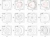 |
Fig. 5. Phase-space portraits (ξ, Pξ) for the model of Eq. (8) with pattern speed Ωsp = 15 km s−1 kpc−1 and density of the spiral potential ρ0 = 5 × 10⁷ M⊙ kpc−3 for 12 different values of the radius rc namely rc = 1, 2, ..., 12 kpc. Precessing ellipses responsible for the spiral density waves are periodic orbits of the x1 family that correspond to radii between approximately 5 kpc (second ILR) and 11 kpc (4:1 resonance). |
Regarding the main families of periodic orbits in the phase portraits of Fig. 5, we refer to the nomenclature of Contopoulos (1975), who called x1, x2 the families of stable and x3 the family of unstable periodic orbits. In our model, the precessing ellipses supporting the spirals are the stable periodic orbits of the x1 family. Four different regions can be distinguished according to the number and stability of periodic orbits: (a) Inside the first ILR, only the x1 family (stable) exists, (b) between the first and the second ILR, three families exist, namely x1, x2 (stable), and x3 (unstable). (c) Between the second ILR and the 4:1 resonance, only the x1 family exists (stable or unstable family), and (d) outside the 4:1 resonance, the x1 family still exists, but it no longer supports the spiral arms (see the Figs. 7, 10, 13, and 16). For Ωsp = 15 km s−1 kpc−1, the second ILR and the 4:1 resonance are approximately at r = 5 kpc and 11 kpc, respectively (Fig. 4). The spirals should thus extend roughly between these two radii.
In the phase portrait of Fig. 5, the x1 family is found at the center of the islands of stability, marked with black points, while the x2 family is at the center of the islands, marked with red points. The unstable periodic orbit x3 is plotted with a blue dot. The orbits x3 exist only in the region between the first and second ILR, and they do not support the imposed spirals (see below). On the other hand, as shown in Fig. 5, the x1 family remains stable at all radii up to the 4:1 resonance. Beyond this resonance, orbits of greater multiplicity bifurcate from the x1 family and substantially affect the structure of the phase space, as in the last panel of Fig. 5.
Figure 6 shows the normalized characteristic curves  (where the epicyclic frequency κc(rc) is given by Eq. (14)) as a function of the radius rc for the same parameters as in Fig. 5. The family x1 is shown in black, x2 in red, and the (unstable) family x3 in blue. We note that the x2 and x3 families exist between the first and second ILR. Both families are created by a tangent bifurcation close to the first ILR, and then rejoin and disappear by inverse bifurcation close to the second ILR. S(rc) in each case represents the amplitude of the epicyclic oscillation of the corresponding (elliptical) periodic orbit.
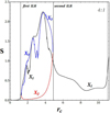 |
Fig. 6. Characteristic curves |

A key remark in Fig. 6 is that in the range of the radii where S(rc) decreases, between the second ILR (at rc ≈ 5 kpc) and rc ≈ 8.5 kpc, the ellipses become more circular, and so they do not intersect with each other. The value of S(rc) reaches a minimum value of about 8.5 kpc and then increases, first smoothly, and then abruptly. After this latter radius, the orbits become rectangular as they approach the 4:1 resonance. Hence, the x1 orbits start intersecting and no longer support the imposed spirals. As a conclusion, the end of the response spiral density wave should be placed somewhere between the radius rc corresponding to the minimum of the curve S(rc) and the 4:1 resonance.
As shown in Fig. 7, the orbits of the x1 family form precessing ellipses supporting the imposed spirals in the whole region between the second ILR (≈5 kpc) and a short distance inside the 4:1 resonance. Figure 7a shows that the x1 family forms a dense and well-defined spiral density wave. In Fig. 7b, the x1 family is plotted both inside and outside the second ILR. Between the first ILR (≈1.5 kpc) and the second ILR (≈5 kpc), the orbits form a more fuzzy spiral density wave, while inside the first ILR, the orbits are more circular. In fact, inside the second ILR, the spiral density wave is greatly weakened because the amplitude of the spiral perturbation is close to zero (see Fig. 1). The imposed spiral arms (superposed in the figure in red) are derived from the minima of the spiral potential of Eq. (8). The coincidence between imposed spirals and those formed by the elliptical orbits is nearly complete.
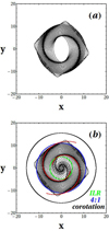 |
Fig. 7. (a) Spiral density waves formed by the precessing ellipses of the elliptical closed orbits of the x1 family, from the model of Eq. (8) for a pattern speed Ωsp = 15 km s−1 kpc−1 and density of the spiral potential ρ0 = 5 × 10⁷ M⊙ kpc−3, between the second ILR and the 4:1 resonance. (b) Same as in (a), but with the ellipses of the x1 family inside the second ILR. Superposed are circles corresponding to the second ILR (green circle), 4:1 resonance (blue circle), and corotation (black circle). The imposed spiral arms (in red) are derived from the minima of the spiral potential of Eq. (8). The coincidence of the imposed spirals with the spiral density wave created by the precessing ellipses is nearly complete. |
4.2. Parametric study
The agreement between the imposed spirals (minima of the potential of Eq. (8)) and the response spirals (formed by the elliptical periodic orbits), as well as the regularity of the phase space structure observed in the previous example, holds for a particular choice of parameters (ρ0, Ωsp, and a). We now study how the above picture is altered by varying independently the amplitude ρ0, the pattern speed Ωsp, or the pitch angle a in the imposed spirals. The results of this parametric study are summarized in Sect. 4.2.3.
4.2.1. Role of the amplitude of the perturbation
In order to investigate the role of the spiral amplitude ρ0 (Eq. (8)), we repeated the study of the previous subsection for increasing values of ρ0. Figure 8 shows the same phase-space portraits (ξ, Pξ) as in Fig. 5, but with ρ0 three times larger (ρ0 = 15 × 107 M⊙ kpc−3). When the amplitude is increased, the main observation is that while the x1 family remains stable for most values of rc, chaos is introduced in the phase space for radii rc > 5 kpc covering a great part of the phase space around the island of stability corresponding to the x1 periodic orbit. The x1 family itself becomes unstable within a small interval of rc values (see Fig. 9). Figure 9 shows the normalized characteristic curves  in the model with ρ0 = 15 × 107 M⊙ kpc−3. As in Fig. 6, here the x2 and x3 periodic orbits are also created together at a tangent bifurcation close to the first ILR, and then they join and disappear close to the second ILR. The value of S(rc) reaches a minimum value around 8.5 kpc (same as in Fig. 6), and then it increases abruptly. Therefore the end of the response spiral density wave here again should be placed somewhere between the radius rc corresponding to the minimum S(rc) and the radius corresponding to the 4:1 resonance.
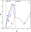 |
Fig. 9. Same as in Fig. 6, but for the density parameter of the spiral potential ρ0 = 15 × 107 M⊙ kpc−3. The dashed part of the black curve denotes the unstable periodic orbit x1. |
Figure 10 shows the spiral density waves generated by the x1 family in this model, extending for radii between the second ILR (rc ≈ 5 kpc) and a short distance inside the 4:1 resonance. The response spirals now appear more concentrated than the spirals in Fig. 7, around the locus of the maximum of the density wave. This is because the forced ellipticity of the x1 orbits increases with ρ0 (see Efthymiopoulos 2010 for a review). In Fig. 10b, the x1 family is plotted both inside and outside the second ILR. Here again, the orbits between the first and second ILR (from ≈1.5 kpc to ≈5 kpc) form a more fuzzy spiral density wave, while inside the first ILR, the orbits are more circular. On the other hand, we again observe a nearly complete coincidence between imposed and response spirals beyond the second ILR. Figure 11 shows the phase portraits (ξ, Pξ) for an even greater (by a factor 6) value of ρ0 = 30 × 107 M⊙ kpc−3. In comparison with Fig. 8, we observe that here chaos is introduced at approximately the same values of rc (i.e., for rc > 5 kpc) as in the previous example. However, the main qualitative difference between these two cases is that in the latter case, the x1 family becomes unstable by a sequence of period-doubling bifurcations starting at rc ≈ 6.8 kpc, and there are no ordered orbits around it from there on. As a consequence, no ordered matter is collected around it that might support a realistic spiral density wave.
Figure 12 shows the normalized characteristic curves  of this model. The main difference with respect to the previous cases is that the curve S(rc) forms a nearly constant plateau from the second ILR to the point rc ≈ 7 kpc and then marks an abrupt fall to a minimum at rc ≈ 8 kpc. As a consequence, the ellipticity of the x1 orbits remains nearly constant in the region between the second ILR and the radius rc ≈ 7 kpc. Moreover, when the elliptical orbits of the unstable x1 periodic orbit are plotted for this model (Fig. 13a), the ellipses intersect each other in the whole range of radii and therefore only define fuzzy spiral density waves (compare with Fig. 10). Some secondary spiral arms also appear. Overall, this is an unrealistic spiral density wave that cannot be observed in real galaxies, as there exists no ordered matter around the x1 family. Fig. 13b shows the same information as Figs. 7b and 10b for ρ0 = 30 × 107 M⊙ kpc−3.
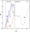 |
Fig. 12. Same as in Fig. 6, but for ρ0 = 30 × 107 M⊙ kpc−3. The dashed part of the black curve denotes that the periodic orbit x1 is unstable. |
Comparing all three models, we find that the precessing ellipses of the x1 family can support the spirals for amplitudes (F-strengths) not exceeding the level 15 − 20%. Beyond this value, the x1 family becomes unstable at a rather small distance beyond the second ILR (Δrc ≈ 2 kpc), while chaos dominates the phase space. This is in accordance with estimates of the amplitude of the spiral perturbation of the spiral arms in real grand-design galaxies, which give a relatively low upper limit (≈10 − 15%) in the forces (Grosbøl & Patsis 1998; Grosbøl et al. 2004). Moreover, long-term evolution of self-gravitating models shows that spiral density waves do not remain viable over many revolutions if the spiral forcing is higher than 5% (Chakrabarti et al. 2003).
For the role of other families of periodic orbits, Fig. 14 shows the precessing ellipses of the x2 family for the model of Eq. (8) for a pattern speed Ωsp = 15 km s−1 kpc−1 and a density of the spiral potential ρ0 = 5 × 10⁷ M⊙ kpc−3 in Fig. 14a, ρ0 = 15 × 107 M⊙ kpc−3 in Fig. 14b, and ρ0 = 30 × 107 M⊙ kpc−3 in Fig. 14c. In all three cases, the response spirals are orthogonal to the response spirals of the x1 family (see Contopoulos 1975). In Figs. 14b and c, they form weak spiral arms in the region between the first and second ILR, where the amplitude of the spiral potential is close to zero (see Fig. 1).
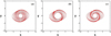 |
Fig. 14. x2 family of orbits for the model of Eq. (8) for (a) a pattern speed Ωsp = 15 km s−1 kpc−1 and density of the spiral potential ρ0 = 5 × 10⁷ M⊙ kpc−3 in (a), ρ0 = 15 × 107 M⊙ kpc−3 in (b) and ρ0 = 30 × 107 M⊙ kpc−3 in (c). In all three cases, these elliptical orbits do not support the spiral wave derived from the galactic potential, and their main axes are perpendicular to the main axes of the x1 family. |
In Fig. 15, some precessing ellipses of the x1 family (black orbits) are plotted together with those of the x2 family (red orbits) for ρ0 = 30 × 107 M⊙ kpc−3 and Ωsp = 15 km s−1 kpc−1, in the range of radii from rc = 2 kpc to rc = 5 kpc. The main axes of the ellipses of the x2 family are perpendicular to the main axes of the x1 family, and they exist for radii for which the amplitude of the spiral perturbation is close to zero (see Fig. 1). Therefore they do not support the spiral density wave. It can easily be verified that the same is true for the unstable x3 family (not shown in the figures).
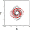 |
Fig. 15. Some precessing ellipses of the x1 family (black orbits) together with the precessing ellipses of the x2 family (red orbits) that correspond to the same radii rc for density of the spiral potential ρ0 = 30 × 107 M⊙ kpc−3 and for a pattern speed Ωsp = 15 km s−1 kpc−1. The main axes of the x2 ellipses are perpendicular to the main axes of the x1 family and do not support the spiral density wave. |
4.2.2. Role of the pattern speed
In order to examine the dependence of the response spiral density wave on the pattern speed Ωsp, we fixed the amplitude of the spiral perturbation to ρ0 = 5 × 10⁷ M⊙ kpc−3 and changed the pattern speed of the spiral potential, comparing the cases Ωsp = 10, 15 and 20 km s−1 kpc−1. Figure 16 shows the spiral density waves formed by the precessing ellipses of the x1 family (black orbits) for the pattern speed Ωsp = 20 km s−1 kpc−1 (in Fig. 16a) and Ωsp = 10 km s−1 kpc−1 (in Fig. 16b). Superposed are the circles corresponding to the ILR radius (green circle), to the 4:1 resonance (blue circle), and to corotation (black circle). By comparing Figs. 16a and b and Figs. 7a and b, which all have the same amplitude ρ0 = 5 × 10⁷ M⊙ kpc−3, but different values of the pattern speed we derive the following conclusions. When the pattern speed decreases, (a) all the resonances are shifted outward (see Fig. 4), and therefore the spiral density waves reach larger radii. However, the ellipses become rounder when they approach the 4:1 resonance, and therefore the spiral density wave becomes less conspicuous at larger radii. (b) The region inside the first ILR becomes smaller, and the region between the first and second ILR increases. The elliptical orbits of the x1 family in this latter region become much more elongated and intersect each other. (c) The width of the spiral arms grows with radius (see Fig. 16b). Savchenko et al. (2020) claimed that in the 86% of a sample of 155 face-on grand-design spiral galaxies, they observed that the arm width increases with radius (see Mosenkov et al. 2020, for an alternative interpretation of this phenomenon based on the mechanism of swing amplification).
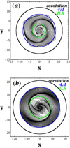 |
Fig. 16. Spiral density waves formed by the elliptical orbits of the x1 family, from the model of Eq. (8) for a pattern speed Ωsp = 20 km s−1 kpc−1 in (a) and Ωsp = 10 km s−1 kpc−1 in (b) and a density of the spiral potential ρ0 = 5 × 10⁷ M⊙ kpc−3. Superposed are circles corresponding to ILR (green circle), 4:1 resonance (blue circle), and corotation (black circle). |
4.2.3. Role of the pitch angle
In this subsection, we chose the model ρ0 = 15 × 107 M⊙ kpc−3, Ωsp = 15 km s−1 kpc−1, but varied the pitch angle from the low value a = −5° to the high value a = −25° instead of the intermediate value a = −13° that was used in all previous numerical experiments.
Figure 17 shows the phase portraits (ξ, Pξ) for a = −25°. By comparing the two figures (8 and 17, which only differ in the value of the pitch angle), we conclude that for an increasing pitch angle (more open spiral arms), more order is introduced in the phase space and the chaotic areas shrink. Therefore more matter exists in ordered motion around the x1 stable periodic orbit that can support the spiral density wave better. The corresponding response spirals (Fig. 19) are also more open and extend throughout the whole region between the second ILR and the 4:1 resonance.
Figure 18 instead shows the phase portraits (ξ, Pξ) when a = −5°. The key observation is that the x1 family now becomes unstable slightly outside the second ILR (at rc ≈ 6.65 kpc) and up to the 4:1 resonance, and the region around it is fully chaotic. This case presents an entirely different behavior than all previous cases. We studied the bifurcations of the x1 and x2 families in this case in the Appendix A in detail. The corresponding spiral density wave formed by the x1 family and its continuation, the b family (of Appendix A), is plotted in Fig. 20a. The ellipses of the x1 family exist up to the second ILR (at rc ≈ 5 kpc) and intersect, forming a rather fuzzy density wave, while the ellipses from the b family (which is the continuation of the x1 family) create a more clearly defined density wave that reaches from the second ILR up to the 4:1 resonance (at rc ≈ 11 kpc). Superposed, in red, are the theoretical minima of the imposed spirals. We observe that they coincide in general with the spiral density wave formed by the precessing ellipses of the x1 family, although a secondary spiral wave appears from a certain radius and beyond. This is an unrealistic spiral density wave as it is formed by unstable periodic orbits of the x1 family that have no ordered matter around them, but only chaotic orbits all the way between the second ILR and the 4:1 resonance. Figure 20b instead shows the spiral density wave formed by the x2 family, which in this model extends far beyond the second ILR (see the Appendix). As commented above, the main axes of the corresponding ellipses are always perpendicular to those of the x1 family ellipses (see Fig. 15), and thus cannot support the imposed spiral arms.
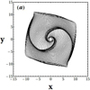 |
Fig. 19. Spiral density wave formed by the precessing ellipses of the x1 family for ρ0 = 15 × 107 M⊙ kpc−3, a pattern speed Ωsp = 15 km s−1 kpc−1, and a pitch angle a = −25°. |
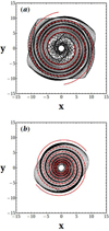 |
Fig. 20. Spiral density waves formed by the precessing ellipses of the (a) x1 family and (b) x2 family for ρ0 = 15 × 107 M⊙ kpc−3, a pattern speed Ωsp = 15 km s−1 kpc−1, and a pitch angle a = −5°. Superposed (in red) is the theoretical spiral derived from the minima of the spiral potential of Eq. (8). |
By comparing Figs. 8, 17, and 18, we conclude that for an increasing pitch angle (more open spiral arms), more order is introduced in the phase space. For very small pitch angles, chaos dominates in the phase space, and we always obtain that the x1 family of orbits becomes unstable almost immediately after the second ILR. The x2 family is also unstable in the region outside the second ILR.
In conclusion, there is a lower limit of the value of the pitch angle a below which the central periodic orbit of the x1 family becomes unstable in the region between the second ILR and the 4:1 resonance. This limit of the pitch angle is defined by the other two free parameters of the model, that is, by the amplitude of the spiral perturbation and the pattern speed of the spiral arm, as indicated in Table 1.
Pitch angle below which the x1 family becomes unstable outside the second ILR for various values of the amplitude of the spiral perturbation and the pattern speed.
Table 1 can be used to estimate the permissible area of pitch angles that for ρ0 and Ωsp as in the first two columns should be larger than the value reported in the third column as a function of the amplitude of the spirals and the pattern speed. From these data, we conclude that using the stability of the x1 family as a criterion, a correlation between the pitch angle and the amplitude of the spiral perturbation suggests that spirals formed by precessing ellipses should be stronger in amplitude when they are more open (larger a). Moreover, a correlation between the pitch angle and the pattern speed is indicated: the higher the value of the pattern speed, the more tightly wound the spirals should be to maintain stability of the x1 family.
4.3. Comparison with observations
In its classical version, the Hubble sequence for spiral galaxies implies that the bulge size and the spiral arm winding should be highly correlated. According to this classification, the “Sa” galaxies have tightly wound arms and fat nuclear bulges, “Sb” galaxies have moderately wound arms and moderate nuclear bulges, and “Sc” galaxies have loosely wound arms and small nuclear bulges. However, modern classification schemes for spiral galaxies imply a considerable departure from the classic Hubble sequence as regards the correlation between spiral arm winding type and bulge size. Early studies suggested that spiral arms become tighter with increasing mass of the bulge (Morgan 1958, 1959; Kennicutt 1981; Bertin et al. 1989). Furthermore, Seigar et al. (2005, 2006) reported a tight connection between pitch angle and morphology of the galactic rotation curve, quantified by the shear rate, with open arms associated with rising rotation curves and tightly wound arms connected to flat and falling rotation curves. On the other hand, Hart et al. (2017) recently analyzed a large sample of galaxies selected from the Sloan Digital Sky Survey (SDSS; York et al. 2000) and found very weak correlations between pitch angle and galaxy mass, and a surprising trend that the pitch angle increases with increasing bulge-to-total mass ratio. Yu & Ho (2019) found that the pitch angle decreases (arms are more tightly wound) in galaxies of earlier Hubble type, more prominent bulges, higher concentration, and higher total galaxy stellar mass. However, there is a significant scatter in their measures. Finally, Masters et al. (2019) and Díaz-García et al. (2019) found little or no correlation between spiral arm winding tightness and bulge size.
There is no concluding evidence of a correlation between the size of the bulge and the pitch angle of the grand design galaxies. We therefore tested various pitch angles in our galactic model and kept the mass of the bulge constant at a relatively high value. The results of the previous subsection indeed suggest a correlation between pitch angle and amplitude of the spiral perturbation, suggesting that galaxies with stronger perturbations should have more open spirals (greater value of the pitch angle). In comparison with real observations, Grosbøl et al. (2002) found that the distribution of mean amplitudes of two-armed spirals as a function of the pitch angle shows a lack of strong in amplitude and at the same time tightly wound spirals. They have also found that most of the mean amplitudes of spiral arms are below 15% in forces, and there is a correlation between the amplitude of spirals and the pitch angle: weak spirals often have tighter spiral arms. Díaz-García et al. (2019) also found that the mean amplitude of the arms increases with increasing pitch angle.
5. Conclusions
We studied the precessing ellipse model of elliptical orbits that support the spiral density waves in grand-design spiral galaxies. We used a theoretical model consisting of a bulge, a disk, a halo, and a spiral potential. The free parameters of our model were the amplitude of the spiral density perturbation (ρ0 in Eq. (8)), the pattern speed of the spiral potential (Ωsp in Eq. (12)), and the pitch angle of the spiral arms of the model (a in Eq. (8)). By testing the effect of the variation in free parameters of the model on the response spirals, formed by elliptical periodic orbits, we extracted the conclusions listed below.
-
(1)
In all models we studied, the x1 family creates response spirals that are consistent with the imposed spirals. The response spirals extend in the region from the center of the galaxy up to the radius of the 4:1 resonance. The x2 and x3 family of orbits exist between the first and second ILR. They are created simultaneously near the first ILR at a tangent bifurcation, and they join and disappear near the second ILR in all the models, except in the case of a very small pitch angle, where they still exist outside the second ILR, but do not contribute to the response spirals. The main axes of the x2 family of orbits are perpendicular to the main axes of the x1 family, and the x3 family is always unstable in the whole range of radii.
-
(2)
By increasing the amplitude of the spiral density perturbation in our model, chaos is introduced gradually and the x1 family of orbits becomes unstable. An upper limit for the spiral density perturbation is ρ0 = 30 × 107 M⊙ kpc−3, where the x1 family is unstable in the whole range between the second ILR and the 4:1 resonance.
-
(3)
When the value of the pattern speed Ωsp decreases, it causes an outward shift of the resonances and therefore the spiral density waves can reach larger radii. However, the ellipses become rounder when they approach the 4:1 resonance, and therefore the spiral density wave becomes less conspicuous at larger radii. Moreover, the elliptical orbits of the x1 family become much more elongated and intersect, thus destroying a coherent spiral response.
-
(4)
We conclude for the value of the pitch angle that for an increasing pitch angle (more open spiral arms), more order is introduced in the phase space and the chaotic areas shrink, while for a decreasing pitch angle (more tight spiral arms), chaos dominates in the phase space and the x1 family of orbits can no longer support the spiral density wave. In the special case of a very small pitch angle, new bifurcations of periodic orbits appear from the main families x1 and x2, but the main bifurcations of the x1 family that cause the spiral density wave become unstable soon after the second ILR, and therefore they cannot support real spirals.
-
(5)
To summarize, the main result of the paper is a quantitative estimation of the range of the free parameters of our galactic model for generating realistic spiral density waves through the precessing ellipses model of elliptical closed orbits (and their surrounding quasi-periodic ones). In particular, a correlation between the pitch angle and the amplitude of the spiral perturbation was shown, where stronger spirals can be statistically less tight than weaker spirals. Moreover, a correlation between the pitch angle and the pattern speed was shown, where spirals that spin faster can be statistically tighter than slower spirals.
Acknowledgments
We acknowledge support by the research committee of the Academy of Athens through the project 200/895.
References
- Athanassoula, E. 1984, Phys. Rep., 114, 319 [Google Scholar]
- Berman, R. H., & Mark, J. W. K. 1977, ApJ, 216, 257 [NASA ADS] [CrossRef] [Google Scholar]
- Bertin, G. 1980, Phys. Rep., 61, 1 [NASA ADS] [CrossRef] [Google Scholar]
- Bertin, G., & Lin, C. C. 1996, Spiral Structure in Galaxies a Density Wave Theory (MA, Cambridge: MIT Press) [Google Scholar]
- Bertin, G., Lin, C. C., Lowe, S. A., & Thurstans, R. P. 1989, ApJ, 338, 78 [CrossRef] [Google Scholar]
- Berry, C. L., & Smet, D. J. 1979, AJ, 84, 964 [NASA ADS] [CrossRef] [Google Scholar]
- Binney, J., & Tremaine, S. 2008, Galactic Dynamics (Princeton University Press) [Google Scholar]
- Block, D. L., Buta, R., Knapen, J. H., et al. 2004, ApJ, 128, 183 [CrossRef] [Google Scholar]
- Buta, R. J., Knapen, J. H., Elmegreen, B. G., et al. 2009, AJ, 137, 4487 [NASA ADS] [CrossRef] [Google Scholar]
- Chakrabarti, S., Laughlin, G., & Shu, F. H. 2003, ApJ, 596, 220 [NASA ADS] [CrossRef] [Google Scholar]
- Chaves-Velasquez, L., Patsis, P. A., Puerari, I., Moreno, E., & Pichardo, B. 2019, ApJ, 871, 79 [CrossRef] [Google Scholar]
- Contopoulos, G. 1970, in The Spiral Structure of Our Galaxy, eds. W. Becker, & G. Contopoulos (Dordrecht: D. Reidel Publishing Co), Proceedings of I.A U. Symposium No 38 [Google Scholar]
- Contopoulos, G. 1971, ApJ, 163, 181 [NASA ADS] [CrossRef] [Google Scholar]
- Contopoulos, G. 1975, ApJ, 201, 566 [NASA ADS] [CrossRef] [Google Scholar]
- Contopoulos, G. J. 1980, JApA, 1, 79 [NASA ADS] [Google Scholar]
- Contopoulos, G. 1985, Comments Astrophys., 11, 1 [NASA ADS] [Google Scholar]
- Contopoulos, G. 2002, Order and Chaos in Dynamical Astronomy (Berlin: Springer) [CrossRef] [Google Scholar]
- Contopoulos, G., & Grosbøl, P. 1986, A&A, 155, 11 [NASA ADS] [Google Scholar]
- Contopoulos, G., & Grosbøl, P. 1988, A&A, 197, 83 [NASA ADS] [Google Scholar]
- Cox, D. P., & Gómez, G. C. 2002, ApJS, 142, 261 [NASA ADS] [CrossRef] [Google Scholar]
- Dehnen, W. 1993, MNRAS, 265, 250 [NASA ADS] [CrossRef] [Google Scholar]
- Díaz-García, S., Salo, H., Knapen, J. H., & Herrera-Endoqui, M. 2019, A&A, 631A, 94 [Google Scholar]
- Dobbs, C., & Baba, J. 2014, PASA, 31, 35 [Google Scholar]
- Donner, K. J., & Thomasson, M. 1994, A&A, 290, 475 [Google Scholar]
- Efthymiopoulos, C. 2010, Eur. Phys. J. Spec. Top., 186, 91 [NASA ADS] [CrossRef] [Google Scholar]
- Efthymiopoulos, C., Harsoula, M.., & Contopoulos, G. 2020, A&A, 636, A44 [NASA ADS] [CrossRef] [EDP Sciences] [Google Scholar]
- Goldreich, P., & Tremaine, S. 1978, ApJ, 222, 850 [NASA ADS] [CrossRef] [Google Scholar]
- Grosbøl, P., & Patsis, P. A. 1998, A&A, 336, 840 [NASA ADS] [Google Scholar]
- Grosbøl, P., Pompei, E., & Patsis, P. A. 2002, ASP Conf. Ser., 275, 305 [Google Scholar]
- Grosbøl, P., Patsis, P. A., & Pompei, E. 2004, A&A, 423, 849 [NASA ADS] [CrossRef] [EDP Sciences] [Google Scholar]
- Hart, R. E., Bamford, S. P., & Hayes, W. B. 2017, MNRAS, 472, 2263 [NASA ADS] [CrossRef] [Google Scholar]
- Junqueira, T. C., Lepine, J. R. D., Braga, C. A. S., & Barros, D. A. 2013, A&A, 550, A91 [NASA ADS] [CrossRef] [EDP Sciences] [Google Scholar]
- Kalnajs, A. J. 1973, PASA, 2, 174 [Google Scholar]
- Kennicutt, R. C. 1981, AJ., 86, 1847 [NASA ADS] [CrossRef] [Google Scholar]
- Lepine, J. R. D., Roman-Lopes, A., Abraham, Z., Junqueira, T. C., & Mishurov, Y. N. 2011, MNRAS, 414, 1607 [NASA ADS] [CrossRef] [Google Scholar]
- Lin, C., & Shu, F. 1964, ApJ, 140, 646 [Google Scholar]
- Lin, C., & Shu, F. 1966, PNAS, 55, 229 [CrossRef] [Google Scholar]
- Lindblad, B. 1940, ApJ, 92, 1 [NASA ADS] [CrossRef] [Google Scholar]
- Lindblad, B. 1955, Stockholm Obs. Ann., 18, 6 [Google Scholar]
- Lindblad, B. 1956, Stockholm Obs. Ann., 19, 7 [NASA ADS] [Google Scholar]
- Lindblad, B. 1957, Stockholm Obs. Ann., 19, 9 [Google Scholar]
- Lindblad, B. 1958, Stockholm Obs. Ann., 20, 4 [Google Scholar]
- Lindblad, B. 1960, Stockholm Obs. Ann., 21, 4 [Google Scholar]
- Lindblad, B. 1961, Stockholm Obs. Ann., 21, 8 [NASA ADS] [Google Scholar]
- Lynden-Bell, D., & Kalnajs, A. J. 1972, MNRAS, 157, 1 [Google Scholar]
- Masters, K. L., Lintott, C. J., Hart, R. E., et al. 2019, MNRAS, 487, 1808 [NASA ADS] [CrossRef] [Google Scholar]
- Mertzanides, C. 1976, A&A, 50, 395 [NASA ADS] [Google Scholar]
- Miyamoto, M., & Nagai, R. 1975, PASJ, 27, 533 [NASA ADS] [Google Scholar]
- Monet, D. G., & Vandervoort, P. O. 1978, ApJ, 221, 87 [NASA ADS] [CrossRef] [Google Scholar]
- Morgan, W. W. 1958, PASP, 70, 364 [NASA ADS] [CrossRef] [Google Scholar]
- Morgan, W. W. 1959, PASP, 71, 394 [NASA ADS] [CrossRef] [Google Scholar]
- Mosenkov, A., Savchenko, S., & Marchuk, A. 2020, Res. Astron. Astrophys., 20, 120 [Google Scholar]
- Norman, C. A. 1978, MNRAS, 182, 457 [CrossRef] [Google Scholar]
- Patsis, P. A., & Grosbøl, P. 1996, A&A, 315, 371 [Google Scholar]
- Patsis, P. A., Contopoulos, G., & Grosbøl, P. 1991, A&A, 243, 373 [NASA ADS] [Google Scholar]
- Patsis, P. A., Hiotelis, N., Contopoulos, G., & Grosbøl, P. 1994, A&A, 243, 373 [Google Scholar]
- Patsis, P. A., Grosbøl, P., & Hiotelis, N. 1997, A&A, 323, 762 [NASA ADS] [Google Scholar]
- Pérez-Villegas, A., Gómez, G. C., & Pichardo, B. 2015, MNRAS, 451, 2922 [CrossRef] [Google Scholar]
- Pettitt, A. R., Dobbs, C. L., Acreman, D. M., & Price, D. J. 2014, MNRAS, 444, 919 [NASA ADS] [CrossRef] [Google Scholar]
- Pichardo, B., Martos, M., Moreno, E., & Espresate, J. 2003, ApJ, 582, 230 [NASA ADS] [CrossRef] [Google Scholar]
- Quillen, A. C., & Minchev, I. 2005, ApJ, 130, 576 [Google Scholar]
- Savchenko, S., Marchuk, A., Mosenkov, A., & Grishunin, K. 2020, MNRAS, 493, 390 [NASA ADS] [CrossRef] [Google Scholar]
- Seigar, M. S., Block, D. L., Puerari, I., Chorney, N. E., & James, P. A. 2005, MNRAS, 359, 1065 [CrossRef] [Google Scholar]
- Seigar, M. S., Bullock, J. S., Barth, A. J., & Ho, L. C. 2006, ApJ, 645, 1012 [NASA ADS] [CrossRef] [Google Scholar]
- Sellwood, J. A. 2010, in Planets Stars and Stellar Systems, ed. G. Gilmore (Heidelberg: Springer), 5 [Google Scholar]
- Sellwood, J. A., & Carlberg, R. G. 1984, ApJ, 282, 61 [Google Scholar]
- Toomre, A. 1964, ApJ, 139, 1217 [Google Scholar]
- Toomre, A. 1977, ARA&A, 15, 437 [NASA ADS] [CrossRef] [Google Scholar]
- Tsigaridi, L., & Patsis, P. A. 2013, MNRAS, 434, 2922 [NASA ADS] [CrossRef] [Google Scholar]
- Vandervoort, P. O. 1971, ApJ, 166, 37 [NASA ADS] [CrossRef] [Google Scholar]
- Vandervoort, P. O. 1973, ApJ, 180, 739 [NASA ADS] [CrossRef] [Google Scholar]
- Vandervoort, P. O., & Monet, D. G. 1975, ApJ, 201, 311 [NASA ADS] [CrossRef] [Google Scholar]
- York, D. G., Adelman, J., & Anderson, J. E. 2000, A&A, 120, 1579 [Google Scholar]
- Yu, S., & Ho, L. 2019, ApJ, 871, 194 [NASA ADS] [CrossRef] [Google Scholar]
- Zhang, X. 2018, Dynamical Evolution of Galaxies (Berlin/Boston: De Gruyter, GmbH) [Google Scholar]
Appendix A: Bifurcations of the orbits in the case of a small pitch angle
Section 4.2.3 describes the case of a very small pitch angle, a = −5°, for the amplitude of the spiral perturbation ρ0 = 15 × 107 M⊙ kpc−3 and a pattern speed Ωsp = 15 km s−1 kpc−1 in our galactic model. In this case, the families of periodic orbits emerge from an intricate sequence of bifurcations. In this appendix, we present some further details of these families.
Figure 18 shows the phase-space portraits of these families for integer values of the radius of the circular orbit rc, namely rc = 1, 2, 3, ..12 kpc. The various bifurcations appear at values of rc between those shown in the figure.
Figure A.1 shows the characteristic curves  of the various families for this case. Fig. A.1a shows the characteristic curve of the x1 family and its bifurcations, while Fig. A.1b shows the characteristic curve of the x2 family and its bifurcations, as well as the x3 family. Figure A.2 shows the phase-space portraits for radii rc = 4.4, 4.5, 4.6, 4.7, 4.78, 4.8, 5.0, and 5.5 kpc, which give a more detailed description of Fig. 18 in the range of radii between rc = 4 and rc = 5.5, where the bifurcations of the x1 and x2 families take place.
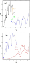 |
Fig. A.1. (a) Characteristic curves |


These figures show that a) for values of rc close to zero, only the stable x1 family exists. This family exists all the way up to rc ≈ 4.84, where it joins the unstable family  and disappears. b) The families x2 (stable) and x3 (unstable) are generated at a tangent bifurcation at rc ≈ 1.2. The family x2 exists all the way up to rc ≈ 8.5, where it joins the unstable family x5 and disappears. The family x3 exists up to rc ≈ 4.98, where it joins the unstable family x4 and disappears. c) The phase-space portrait (ξ, Pξ) for rc = 4.4 (Fig. A.2a) shows x1, x2, x3, and some new bifurcated orbits inside the domain covered by red invariant curves, surrounding the x2 periodic orbit. These orbits are called b (blue stable periodic orbit) and g (green unstable periodic orbit) and have been generated at rc ≈ 4.23 at a tangent bifurcation (Fig. A.1a). Fig. A.2a also clearly shows that the separatrix from x3 surrounds x2 (inner curve of separatrix) and both x1 and x2 (outer curve of separatrix). d) From Fig. A.2b (rc = 4.5), we conclude that for a slightly smaller rc, the unstable periodic orbit g has moved downward and has reached the separatrix emanating from x3. e) Fig. A.2c (rc = 4.6) shows that the separatrix of g surrounds both the x1 and the b periodic orbits. The separatrix of x3 no longer surrounds the orbit b. f) For rc = 4.6 (Fig. A.2c), two new orbits appear in the domain around the x2 periodic orbit, namely orbits x4 (stable) and x5 (unstable) created at a tangent bifurcation at rc ≈ 4.51 (Fig. A.1b). The separatrix emanating from x5 surrounds both x2 and x4. Moreover, the separatrix of x3 surrounds all the three orbits, namely x2, x4, and x5. g) Fig. A.2d (rc = 4.7) shows that two more families of orbits are created inside the region surrounding the x1 periodic orbit, namely
  (stable) and
  (unstable). These families are generated at a tangent bifurcation at rc ≈ 4.64 (Fig. A.1a). h) Fig. A.2e (rc = 4.78) shows that the separatrix emanating from x3 has almost reached the unstable orbit x5 and the separatrix emanating from x5 (that surrounds x4) has almost reached x3. For a slightly smaller value of rc, these parts of the two separatrices should coincide. i) At rc = 4.8 (Fig. A.2f), the separatrix emanating from x3 surrounds only x4. On the other hand, the separatrix emanating from x5 surrounds on the one side the periodic orbit x2 and the other side all the periodic orbits
  , and g. j) At rc ≈ 4.98, the orbits x3 and x4 join and disappear, and the same happens for orbits x1 and
  at rc ≈ 4.84 (Figs. A.1a,b). Thus, for rc = 5 (Fig. A.2g), only the periodic orbits
  (stable), b (stable), g (stable), x2 (stable), and x5 (unstable) exist. k) At rc ≈ 5.45, the orbits
  and g join and vanish (Fig. A.1a). Thus, for rc = 5.5 (Fig. A.2h), only orbits b (stable), x2 (stable), and x5 (unstable) remain. l) At rc ≈ 8.5, families x2 and x5 join and vanish (Fig. A.1b), and finally, beyond rc ≈ 8.5 only the b periodic orbit remains up to the 4:1 resonance. This is the main family that could support the spiral density wave, but it is unstable in most of the domain between the second ILR and the 4:1 resonance. Although we have constructed a density wave out of the precessing ellipses of the unstable periodic orbit b (see Fig. 20a), the fact that there are no ordered orbits around this periodic orbit, has as a result that such a spiral density wave cannot be observed in real galaxies.
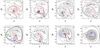 |
Fig. A.2. Phase-space portraits (ξ, Pξ) for the model of Eq. (8) with pattern speed Ωsp = 15 km s−1 kpc−1, ρ0 = 15 × 107 M⊙ kpc−3, and a = −5°, for values of the radius rc = 4.4, 4.5, 4.6, 4.7, 4.78, 4,8, 5.0, and 5.5 kpc. Precessing ellipses responsible for the spiral density waves are periodic orbits of the b family (bifurcation of the x1 family). |
The sequence of bifurcations that we observe in Figs. A.1a and b is much more complicated than in the corresponding Figs. 6, 9, and 12, where only families x1, x2 and x3 exist. In these cases, families x2 and x3 start at a tangent bifurcation and disappear by joining again. Family x1 is stable all the way to the 4:1 resonance and beyond it for a small amplitude of the spiral perturbation (ρ0 = 5 × 10⁷ M⊙ kpc−3, Fig. 5), but it becomes unstable at a certain radius between the second ILR and the 4:1 resonance by a sequence of period-doubling bifurcations for higher values of the amplitudes, that is, for ρ0 ⩾ 15 × 107 M⊙ kpc−3 (see Figs. 8 and 11).
In all these cases, the pitch angle is a = −13°. For larger pitch angles (see Fig. 16 for a = −25°), the x1 family is stable at least up to the 4:1 resonance.
In the present case, where the pitch angle is significantly smaller, that is, a = −5°, family x1 has a very different evolution. The characteristic curve of x1 (stable) is continued by the characteristic curve of  (unstable and backward in rc), then
  (stable and forward in rc), g (unstable and backward in rc), and b (stable and forward in rc) (Fig. A.1a), which finally becomes unstable by a period-doubling bifurcation slightly after rc ≈ 6 and produces great chaos. On the other hand, the characteristic curve of x3 (unstable) starts at tangent bifurcation with x2 (stable) and continues with the characteristic curve of x4 (stable, backward in rc), the x5 (unstable), and finally, it joins x2 (stable) at rc ≈ 8.5 and disappears. Thus the extended characteristic curves of x3 and x2 have the same starting and ending points as in all the previous models.
Another strange new feature in this model is the evolution of the separatrices of the new unstable families g and x5. In both cases, the unstable points of g and x5 reach the separatrix emanating from the unstable point x3 at critical values of rc = rccrit. After this value of rc, the separatrices emanating from g or x5 change drastically.
All Tables
Pitch angle below which the x1 family becomes unstable outside the second ILR for various values of the amplitude of the spiral perturbation and the pattern speed.
All Figures
|
Fig. 1. Total force perturbation Fall for different amplitudes of the spiral potential as a function of the radius. |
| In the text | |
|
Fig. 2. (a) Surface density profile of the axisymmetric part of the model. The green curve represents the bulge, the blue curve represents the disk, and the black curve is the total profile. (b) Rotation velocity curve produced by the axisymmetric potential Vax. |
| In the text | |
|
Fig. 3. Isodensities of the projected surface density of the 3D galactic model (see text). Superimposed are the spiral arms derived from the minima of the spiral potential of Eq. (8). |
| In the text | |
|
Fig. 4. Form of the function Ω(r) and of the resonant combinations of Ω(r) and κ(r), Ω − κ/2, Ω + κ/2, and Ω − κ/4. The selected pattern speed Ωsp determines the radii of the ILR, the 4:1 resonance, and the corotation. |
| In the text | |
|
Fig. 5. Phase-space portraits (ξ, Pξ) for the model of Eq. (8) with pattern speed Ωsp = 15 km s−1 kpc−1 and density of the spiral potential ρ0 = 5 × 10⁷ M⊙ kpc−3 for 12 different values of the radius rc namely rc = 1, 2, ..., 12 kpc. Precessing ellipses responsible for the spiral density waves are periodic orbits of the x1 family that correspond to radii between approximately 5 kpc (second ILR) and 11 kpc (4:1 resonance). |
| In the text | |
|
Fig. 6. Characteristic curves |
| In the text | |
|
Fig. 7. (a) Spiral density waves formed by the precessing ellipses of the elliptical closed orbits of the x1 family, from the model of Eq. (8) for a pattern speed Ωsp = 15 km s−1 kpc−1 and density of the spiral potential ρ0 = 5 × 10⁷ M⊙ kpc−3, between the second ILR and the 4:1 resonance. (b) Same as in (a), but with the ellipses of the x1 family inside the second ILR. Superposed are circles corresponding to the second ILR (green circle), 4:1 resonance (blue circle), and corotation (black circle). The imposed spiral arms (in red) are derived from the minima of the spiral potential of Eq. (8). The coincidence of the imposed spirals with the spiral density wave created by the precessing ellipses is nearly complete. |
| In the text | |
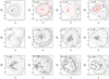 |
Fig. 8. Same as Fig. 5, but for ρ0 = 15 × 107 M⊙ kpc−3. |
| In the text | |
|
Fig. 9. Same as in Fig. 6, but for the density parameter of the spiral potential ρ0 = 15 × 107 M⊙ kpc−3. The dashed part of the black curve denotes the unstable periodic orbit x1. |
| In the text | |
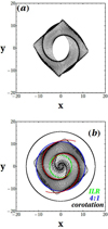 |
Fig. 10. Same as in Fig. 7, but for ρ0 = 15 × 107 M⊙ kpc−3. |
| In the text | |
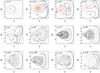 |
Fig. 11. Same as Fig. 5, but for ρ0 = 30 × 107 M⊙ kpc−3. |
| In the text | |
|
Fig. 12. Same as in Fig. 6, but for ρ0 = 30 × 107 M⊙ kpc−3. The dashed part of the black curve denotes that the periodic orbit x1 is unstable. |
| In the text | |
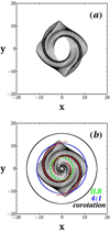 |
Fig. 13. Same as in Fig. 7, but for ρ0 = 30 × 107 M⊙ kpc−3. |
| In the text | |
|
Fig. 14. x2 family of orbits for the model of Eq. (8) for (a) a pattern speed Ωsp = 15 km s−1 kpc−1 and density of the spiral potential ρ0 = 5 × 10⁷ M⊙ kpc−3 in (a), ρ0 = 15 × 107 M⊙ kpc−3 in (b) and ρ0 = 30 × 107 M⊙ kpc−3 in (c). In all three cases, these elliptical orbits do not support the spiral wave derived from the galactic potential, and their main axes are perpendicular to the main axes of the x1 family. |
| In the text | |
|
Fig. 15. Some precessing ellipses of the x1 family (black orbits) together with the precessing ellipses of the x2 family (red orbits) that correspond to the same radii rc for density of the spiral potential ρ0 = 30 × 107 M⊙ kpc−3 and for a pattern speed Ωsp = 15 km s−1 kpc−1. The main axes of the x2 ellipses are perpendicular to the main axes of the x1 family and do not support the spiral density wave. |
| In the text | |
|
Fig. 16. Spiral density waves formed by the elliptical orbits of the x1 family, from the model of Eq. (8) for a pattern speed Ωsp = 20 km s−1 kpc−1 in (a) and Ωsp = 10 km s−1 kpc−1 in (b) and a density of the spiral potential ρ0 = 5 × 10⁷ M⊙ kpc−3. Superposed are circles corresponding to ILR (green circle), 4:1 resonance (blue circle), and corotation (black circle). |
| In the text | |
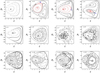 |
Fig. 17. Same as in Fig. 8, but for a pitch angle a = −25°. |
| In the text | |
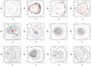 |
Fig. 18. Same as in Fig. 8, but for a pitch angle a = −5°. |
| In the text | |
|
Fig. 19. Spiral density wave formed by the precessing ellipses of the x1 family for ρ0 = 15 × 107 M⊙ kpc−3, a pattern speed Ωsp = 15 km s−1 kpc−1, and a pitch angle a = −25°. |
| In the text | |
|
Fig. 20. Spiral density waves formed by the precessing ellipses of the (a) x1 family and (b) x2 family for ρ0 = 15 × 107 M⊙ kpc−3, a pattern speed Ωsp = 15 km s−1 kpc−1, and a pitch angle a = −5°. Superposed (in red) is the theoretical spiral derived from the minima of the spiral potential of Eq. (8). |
| In the text | |
|
Fig. A.1. (a) Characteristic curves |
| In the text | |
|
Fig. A.2. Phase-space portraits (ξ, Pξ) for the model of Eq. (8) with pattern speed Ωsp = 15 km s−1 kpc−1, ρ0 = 15 × 107 M⊙ kpc−3, and a = −5°, for values of the radius rc = 4.4, 4.5, 4.6, 4.7, 4.78, 4,8, 5.0, and 5.5 kpc. Precessing ellipses responsible for the spiral density waves are periodic orbits of the b family (bifurcation of the x1 family). |
| In the text | |
Current usage metrics show cumulative count of Article Views (full-text article views including HTML views, PDF and ePub downloads, according to the available data) and Abstracts Views on Vision4Press platform.
Data correspond to usage on the plateform after 2015. The current usage metrics is available 48-96 hours after online publication and is updated daily on week days.
Initial download of the metrics may take a while.