| Issue |
A&A
Volume 655, November 2021
|
|
|---|---|---|
| Article Number | A96 | |
| Number of page(s) | 11 | |
| Section | Stellar structure and evolution | |
| DOI | https://doi.org/10.1051/0004-6361/202140701 | |
| Published online | 25 November 2021 | |
Exploring the accretion-ejection geometry of GRS 1915+105 in the obscured state with future X-ray spectro-polarimetry
1
Department of Physics, Tor Vergata University of Rome, Via della Ricerca Scientifica 1, 00133 Rome, Italy
e-mail: This email address is being protected from spambots. You need JavaScript enabled to view it.
2
INAF – IAPS, Via Fosso del Cavaliere 100, 00133 Rome, Italy
3
Dipartimento di Matematica e Fisica, Universita degli Studi Roma Tre, Via della Vasca Navale 84, 00146 Roma, Italy
4
INAF – Astronomical Observatory of Rome, Via Frascati 33, 00078 Monte Porzio Catone, Rome, Italy
5
INFN – Tor Vergata, Via della Ricerca Scientifica 1, 00133 Rome, Italy
6
Department of Astronomy, University of Maryland, College Park, MD 20742, USA
7
NASA/Goddard Space Flight Center, Greenbelt, MD 20771, USA
8
INFN-Pisa, Largo B. Pontecorvo 3, 56127 Pisa, Italy
Received:
2
March
2021
Accepted:
31
August
2021
Abstract
Context. GRS 1915+105 has been in a bright flux state for more than two decades, but in 2018 a significant drop in flux was observed, partly due to changes in the central engine along with increased X-ray absorption.
Aims. The aim of this work is to explore how X-ray spectro-polarimetry can be used to derive the basic geometrical properties of the absorbing and reflecting matter. In particular, the expected polarisation of the radiation reflected off the disc and the putative outflow is calculated.
Methods. We used NuSTAR data collected after the flux drop to derive the parameters of the system from hard X-ray spectroscopy. The spectroscopic parameters were then used to derive the expected polarimetric signal, using results from a Monte Carlo radiative transfer code, both in the case of neutral and fully ionised matter.
Results. From the spectral analysis, we find that the continuum emission becomes softer with increasing flux, and that in all flux levels the obscuring matter is highly ionised. This analysis, on the other hand, confirms that spectroscopy alone is unable to put constraints on the geometry of the reflectors. Simulations show that X-ray polarimetric observations, such as those that will be provided soon by the Imaging X-ray Polarimetry Explorer (IXPE), will help to determine the geometrical parameters which are left unconstrained by the spectroscopic analysis.
Key words: accretion, accretion disks / stars: winds, outflows / X-rays: binaries / polarization / relativistic processes
© ESO 2021
1. Introduction
GRS 1915+105 is a low mass X-ray binary (LMXB), hosting a black hole of mass 12.4 M⊙ and a K1 star (Boeer et al. 1996; Reid et al. 2014). The high luminosity and the extreme variability in the light curves and spectra seen (Belloni et al. 2000) in this system make it a unique source to study the accretion-ejection phenomena in galactic black hole binaries (BHBs).
State changes are a common feature in BHBs. In general the spectral states can be classified as high-soft (HS) and low-hard (LH; Belloni et al. 2000). Some BHBs, especially transient ones, exhibit hysteresis in their hardness intensity diagram (HID), initially rising from an LH state and later transiting towards an HS state (Fender et al. 2004). At times, a jet is observed in the radio band during the hard state and also during the transition to the soft state (Fender et al. 2004). GRS 1915+105 properties differ from those of other transient BHBs, probably due to a large accretion disc. Even though GRS 1915+105 does not exhibit hysteresis in the HID, as persistent BHBs such as Cygnus X-1, Cygnus X-3, hard-soft transitions are seen (Belloni et al. 2000; Vrtilek & Boroson 2013; Zdziarski et al. 2016). An anti-correlation between jet and accretion disc wind was reported in GRS 1915+105 (Neilsen & Lee 2009), such that in observations where wind was present the jet was weak or absent, and in states where the jet was present the wind was weak or absent. This suggested that the disc outflowing in the form of winds could play a role in the state transitions in these systems. The state dependence of the accretion disc wind is not clearly understood at present, as there exist multiple mechanisms responsible for a disc wind and the predominant mechanism might differ depending on the state. In GRS 1915+105, magneto hydro-dynamical modelling (MHD) of the wind indicated that the density of the wind in a soft state is two orders of magnitude higher than in a hard state (Ratheesh et al. 2021). A similar analysis in some other BHBs is currently under progress (Fukumura et al. 2020). Hence, probing the role played by outflows in state transitions needs a clear understanding of the disc-jet-wind connection in different states.
Interestingly, since March 2018, GRS 1915+105 entered into a novel state. In fact, the source intensity started to decline gradually, while the hardness ratio increased indicating a spectral hardening (Koljonen & Tomsick 2020). The source showed the presence of absorption lines during this period (Miller et al. 2020; Balakrishnan et al. 2021). Furthermore, in 2019, the flux dropped sharply into a obscured state (OS) with reflected emission lines seen in the X-ray spectra (Miller et al. 2020). In this faint state, a clear increase in the intrinsic absorption is apparent, making the source a Galactic equivalent of highly absorbed active galactic nuclei (AGN) at times (Miller et al. 2020). Heavy absorption seen in high mass X-ray binaries (HMXBs) is understood to be due to the stellar wind (Kaper et al. 1993; Oskinova et al. 2012). However, in the case of low mass X-ray binaries (LMXBs), the absorption could originate from the environment around the compact object making this a peculiar state in the accretion-ejection regime. There are different sources of obscuration in X-ray binaries, such as slim discs (Motta et al. 2017), optically thick accretion wind (Middleton et al. 2021; Miller et al. 2020), a vertically extended outer disc (GRS 1915+105: Neilsen et al. 2020), among others. One of the main possible candidates in GRS 1915+105 could be a failed magnetic wind (Miller et al. 2020), as magnetic winds are seen close to the central engine in X-ray binaries (Miller et al. 2015, 2016; Fukumura et al. 2017; Ratheesh et al. 2021).
GRS 1915+105 has a high inclination angle of 66° ± 2° (Fender et al. 1999) with a large accretion disc, making it an ideal system to study the reprocessing of the continuum in the accretion disc winds. Accretion disc winds are preferentially seen at high inclination angles, indicating high column density in the equatorial direction (Ponti et al. 2012). GRS 1915+105 is known to have very strong absorption lines in its X-ray spectra (Ueda et al. 2009; Neilsen & Lee 2009; Miller et al. 2015, 2016). While transiting into the OS, the source was also seen in an intermediate state showing the presence of strong absorption lines predominantly at 6 to 7 keV (Koljonen & Tomsick 2020; Miller et al. 2020; Neilsen et al. 2020). The OS has strong emission lines (Miller et al. 2020), indicating reflection from either a distant disc, wind, or a torus. Spectroscopic data suggest that the obscurer could be a failed disc wind (Miller et al. 2020). In OS, GRS 1915+105 has a flux of an order of magnitude lower than in the previous states. Sporadic X-ray flares are also observed in this state (Iwakiri et al. 2019; Neilsen et al. 2019; Jithesh et al. 2019), unlike the kind of variability seen in the source before. Strong radio flares are also seen during this unusual state, even though any correlation of X-ray and radio flares are currently under investigation (Motta et al. 2019; Trushkin et al. 2020). Koljonen & Tomsick (2020) indicate that the source becomes partially obscured in this state with a hardening of the spectral index, as also suggested by Miller et al. (2020) indicating a change in the central engine properties. Koljonen & Tomsick (2020) further suggest that the source could be going into a hard state with a low Eddington luminosity of 1−2%, but the strong radio flares suggest that the accretion rate has not reduced to a large extent. However, high radiative efficiency could be another possibility for the radio flares instead of the change in the accretion rate.
It has long been recognised that the structure of the absorbing matter in AGN, and in particular in Compton-thick ones, can be constrained by X-ray polarimetry (e.g. Goosmann & Matt 2011). With the upcoming launch of NASA/ASI’s Imaging X-ray Polarimetry Explorer (IXPE) in late 2021, the X-ray polarimetric window will be opened (Weisskopf et al. 2016). The gas pixel detectors on board IXPE will be sensitive to polarisation in the 2−8 keV range (Costa et al. 2001). Polarimetry promises to break model degeneracies remaining after spectral and timing model analyses. In fact, different physical and geometrical models can produce similar spectral shapes, however their signatures in polarisation might be different. For example a spherical or a slab geometry of the corona of a compact object would have significantly different polarisation properties (Schnittman & Krolik 2010). Similarly the geometry of the reflecting matter can also be probed using polarimetry.
Estimating the continuum emission in the OS requires broadband hard X-ray spectroscopy up to a few tens of kiloelectron volt as provided by NuSTAR, which will also help to disentangle the continuum from the reflection features. In this paper, we analyse NuSTAR observations of GRS1915+105 taken after the source entered into the OS to derive the main physical properties of the obscuring matter, as well as its geometrical parameters as far as can be constrained by spectroscopy alone. We perform a flux resolved spectral analysis of the OS of GRS 1915+105 using relativistic reflection and absorption models. We also derive the expected polarimetric properties in X-rays for various spectral and geometrical parameters and then apply it to the case of the OS of GRS 1915+105. This paper is organised in the following manner. In Sect. 2 we outline the justification for the selection of NuSTAR data and data reduction methods. Section 3 contains results of the spectral analysis of NuSTAR data at different flux levels. Section 4 contains the results of polarimetric simulations using the radiative transfer code for a toy model and we derive its applications to the OS of this source. In Sect. 5, we summarise and discuss the findings from this work, compare our results with previous ones, and present and discuss the feasibility of IXPE observations to constrain the geometry of the system.
2. Data selection and reduction
Daily monitoring of the X-ray sky has been possible due to the Burst Alert Telescope on board the Neil Gehrels Swift Observatory (Swift/BAT: Krimm et al. 2013) and Gas Slit Camera on board Monitor of All-sky X-ray Image (MAXI/GSC: Matsuoka et al. 2009) in hard (15−50 keV) and soft X-ray (2−20 keV) bands, respectively. We used the Swift/BAT light curves (15−50 keV) obtained from the Swift/BAT transient database1 and MAXI/GSC light curves (2−20 keV) obtained from MAXI/GSC web page2 of GRS 1915+105 to determine the epoch at which the source faded into a low flux state (Fig. 1). The light curves plotted in Fig. 1 were normalised by the Crab count rate in the respective energy bands. The Crab count rates for energies 2−20 keV, 2−4 keV, and 10−20 keV in MAXI/GSC are 3.43 c s−1 cm−2, 1.90 c s−1 cm−2, and 0.36 c s−1 cm−2, respectively, and for energy 15−50 keV in Swift/BAT the count rate is 0.22 c s−1 cm−2. The flux dropped around MJD 58600 and the change in the flux is also linked to the hardening of the spectra, which is seen in the HID in Fig. 2. In the OS, the source count rate in is 0.01 to 0.03 Crab with a hardness ratio greater than 2.5. During the transition to a heavy OS, the source was also in a partial OS with the presence of a strong absorption line as previously reported by Koljonen & Tomsick (2020), and Neilsen et al. (2020).
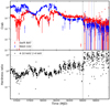 |
Fig. 1. Top: Swift/BAT and MAXI/GSC daily averaged light curves in energy range 15−50 keV and 2−20 keV, respectively. The red, blue, and black vertical lines denote the NuSTAR observations used in this work. The black dotted line roughly indicates the epoch at which the source enters the obscured state (OS). The flux is normalised to crab units. Bottom: evolution of hardness ratio (4−10 keV/2−4 keV) with time in MAXI/GSC. |
NuSTAR observed GRS 1915+105 multiple times after the state transition into a low flux state. However in this work we concentrate on only three archived target of opportunity (ToO) observations taken while the source was in an extremely absorbed state. The observations used in this analysis were performed on July 31, 2019 (NuSTAR obsID:30502008004, from now on obsID1), September 13, 2019 (NuSTAR obsID:30502008006, from now on obsID2), and October 16, 2019 (NuSTAR obsID:90501346002, from now on obsID3) for an exposure of 23.2 ks, 23.7 ks, and 42.6 ks, respectively. The red, blue, and black vertical lines in the top panel of Fig. 1 represent the MJD of obsID1, obsID2, obsID3, respectively. They are also marked as distinct points in Fig. 2 from the MAXI/GSC data on the MJD of these observations. The NuSTAR data of GRS 1915+105 were reduced using v.0.4.6 of the NuSTARDAS pipeline with NuSTAR CALDB v.20200526. The nupipeline tool was used to generate cleaned event files. The source and the background for further analysis were selected manually using a circular region in the image using DS9 (Joye & Mandel 2003). The source region was centred at the source location, and the background was selected away from the source to avoid contamination from the source. The radius of the circular region was determined manually to include maximum source photons in the case of the source and to exclude source contamination in the case of the background (the radius used for obsID1 is 57″, for obsID2 it is 55″, and for obsID3 it is 56″). The nuproducts tool was used to extract a source background subtracted spectrum and light curve for the selected regions. The light curves of these observations from both FPMA and FPMB in the 3−79 keV energy range and binned at 10 s are shown in Fig. 3. The light curves show a large variation in the count rate as also previously reported by Iwakiri et al. (2019), Neilsen et al. (2019), and Jithesh et al. (2019).
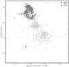 |
Fig. 2. Hardness intensity diagram (HID) made using daily averaged MAXI/GSC light curves. The black and grey points indicate the data points before and after the transition epoch. The coloured points are during the MJD of the observations used in this work. |
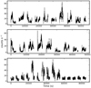 |
Fig. 3. NuSTAR/FPMA light curves in the 3−79 keV energy band. Top, middle, and bottom: represent obsID1, obsID2, and obsID3, respectively. The light curve is plotted from the start time of the observation and was binned at 10 s. |
3. Spectral analysis
The spectral fitting was performed using XSPEC version 12.10.1 (Arnaud 1996; Dorman et al. 2003). The spectra from both FPMA and FPMB were grouped using the grppha module of the FTOOLS (NASA High Energy Astrophysics Science Archive Research Center (HEASARC) 2014) in such a way that each bin contains a minimum of 25 counts. As an initial probe, we modelled the spectra in the 3−79 keV range in all observations using a cutoff power-law (cutoffpl), along with galactic absorption (tbabs: Wilms et al. 2000) and a constant (const) to account for uncertainties between FPMA and FPMB. Since the goal of the initial test was to model the continuum, we excluded the reflection-dominated energy ranges of 5 − 7.5 keV and 12 − 40 keV. The neutral hydrogen column density (NH) was fixed at 5.0 × 1022 cm−2 as previously seen in this source (Zoghbi et al. 2016; Koljonen & Tomsick 2020). We used the χ2 statistics to determine the goodness of the fit throughout this work. For the initial fit, we got a χ2/d.o.f. of 1560/481, 1277/443, and 3070/545 for obsID1, obsID2, and obsID3, respectively. We then used the estimated continuum to plot the spectra and residuals in the 3−79 keV interval to highlight the Gaussian Fe Kα feature at 6.5 keV and a Compton hump at 10−50 keV as signatures of reflection often seen in BHBs. The spectrum and the residuals are shown in Fig. 4. The photon index of the fit resulted in unusually low values of 0.81, 0.61, and 0.83 for obsID1, obsID2, and obsID3, respectively, suggesting that the spectra are reflection-dominated and the continuum is highly absorbed. With different combinations of relativistic reflection models and ionised absorbers, we did not get a reasonable fit. This could be due to the variability in the spectral parameters along with the variability seen as flares in the light curves. Hence, we performed a flux resolved spectroscopic analysis as outlined in the next sub-sections.
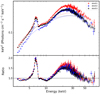 |
Fig. 4. Unfolded NuSTAR spectra of obsID1 (red), obsID2 (blue), obsID3 (black) modelled with the cutoffpl and galactic absorption for plotting purposes. The fitted models are shown by dotted lines in their respective colours. The plots shows only FPMA data. |
3.1. Flux resolved spectroscopy
We divided the three observations into four different flux levels and combined similar flux levels from different observations. The main aim of this method is to explore if there is a change in any of the spectral parameters with respect to the flux. If there is a change, either in the spectral parameters or the geometry of the absorber and reflector, then we can expect a respective change in the polarisation degree and angle. The time intervals for flux resolved spectra were selected from a 10 s binned light curve of FPMA. The flux levels correspond to count-rate intervals of < 15 c s−1, 15−30 c s−1, 30−40 c s−1, and > 40 c s−1. This corresponds to an average flux of 8.07, 15.83, 22.93, and 30.56 × 10⁻¹⁰ ergs cm−2 s−1 in the 3−50 keV range. We generated good time intervals (GTIs) for different flux levels and re-generated the spectra in those time intervals using nuproducts. We combined the respective spectra using the addspec tool (version 1.3.0) of FTOOLS. Before combining the fit, we also verified that the spectra from the same flux levels from different observations are consistent with each other.
We modelled all the spectra using a Comptonisation model (nthcomp: Zdziarski et al. 1996; Życki et al. 1999), two reflection models for the reflection from the accretion disc and the obscurer (xillverCP, García & Kallman 2010; García et al. 2011, 2013), galactic absorption (tbabs: Wilms et al. 2000), and a multiplicative ionised absorber (zxipcf: Reeves et al. 2008; Miller et al. 2006) on the direct continuum and on the disc reflector. The neutral absorption NH was frozen at 5.0 × 1022 cm−2 for all the observations and a constant was used to account for the uncertainties in the calibration between FPMA and FPMB, as mentioned in the initial fit. Hence the final model in XSPEC notation is const × tbabs × (zxipcf × (nthcomp+xillverCP1) + xillverCP2). Here we assume the xillverCP1 to be the disc component and xillverCP2 to be the wind. The assumed geometry of the spectral model is shown in Fig. 5. Here the reflected component from the wind could either be from the side towards the line of sight or on the other side. We find an excess above 50 keV, which may be connected to a putative jet emission (Kong et al. 2021). We do not focus on its origin here and it did not affect our spectral modelling, which is dominated by the spectrum below 20 keV. The covering fraction in zxipcf was frozen to 1.0 as it was found to always be consistent with unity. We used a disc black body as a seed in the nthcomp Comptonisation model. Since the spectra in the NuSTAR energy range are not very sensitive to the seed black body temperature, we fixed it at 0.8 keV which is a reasonable value for the hard state of GRS 1915+105. We used xillverCP to model the reflection component only, and hence we tied the electron temperature and photon index within the xillverCP model to the same parameters in nthcomp. However, to compute the reflected spectrum, xillverCp uses a nthcomp model with a seed black body temperature of 0.05 keV, which might cause some uncertainties in the model especially in soft X-rays below 5 keV. When left free, the iron abundance (AFe) was constrained between 2.0 and 3.0 and we fixed AFe to 2.5. Super solar iron abundances were seen previously in this source (Lee et al. 2002; Ueda et al. 2009; Kong et al. 2021). The inclination angle of the system has been estimated to be 66° ± 2° (Fender et al. 1999), so we fixed the disc inclination to this value. We also fixed the wind inclination angle to 30°, since this parameter was insensitive to the fit. The ‘refl_frac’ in xillver, which is defined as the ratio of the flux incident on the disc to the flux escaping into the line of sight (Dauser et al. 2016), was also frozen to 1 as this parameter was poorly constrained in the fit. We also calculated the ratio of the flux of reflected components to that of the continuum in 2−8 keV (Rsoft) and 10−50 keV (Rhard) energy intervals to understand if the intrinsic flux is dominated by the reflected component in comparison to the direct continuum. The parameters of the fit are outlined in Table 1, and Fig. 6 shows the modelled spectra of all observations. Figure 7 shows the unabsorbed continuum and both the reflectors at different flux levels.
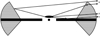 |
Fig. 5. Geometry assumed for the best fit spectral model as outlined in the text. We note that 1, 2, and 3 represent reflection from the disc, continuum emission, and reflection from the wind, respectively. The continuum is assumed to originate from the corona above the black hole. The shaded portion indicates the disc wind, while the black horizontal structure represents the disc. |
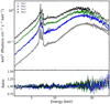 |
Fig. 6. Unfolded NuSTAR spectra for different flux levels as outlined in Sect. 3. The colours grey, blue, green, and black represent flux 1, flux 2, flux 3, and flux 4, respectively. The plots shows only FPMA data. |
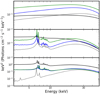 |
Fig. 7. Unabsorbed spectral components at different flux levels. Top: nthcomp. Middle: xillverCP2 – wind. Bottom: xillverCP1 – disc. The colours grey, blue, green, and black represent flux 1, flux 2, flux 3, and flux 4, respectively. |
Parameters of the spectral fit from flux resolved spectroscopy.
The parameters from the spectral fit are plotted with respect to the flux in Fig. 8. The main finding is that the photon index is correlated to the flux. The electron temperature is also seen to increase after a drop from the first to the second flux level. This indicates that the flux change is correlated to changes in the central engine. We find that the properties of the ionised absorber do not change with respect to the flux (see Fig. 8). The ionisation parameters of the disc and wind reflectors are in the range of 102 to 104 erg s−1 cm and 103 to 105 erg s−1 cm, respectively. We also see an increase in the red shift with respect to the flux for the wind reflector, while no clear trend is seen for the red shift of the disc component. Other than the highest flux level, the Rhard is constant, while in the highest flux level, Rhard increased by an order of magnitude for the disc and by a factor of 5 for the wind.
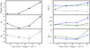 |
Fig. 8. Spectral parameters from the flux resolved spectroscopy with respect to the flux. The colours black, grey, blue, and green represent the spectral parameters of the continuum (nthcomp), ionised absorber (zxipcf), wind reflector (xillverCP1), and disc reflector (xillverCP2), respectively. Left: top, middle, and bottom: photon index, electron temperature, and NH of the ionised absorber, respectively. Right: top, middle, and bottom: ionisation parameter, red shift, and Rhard, respectively. |
These spectral models and results from our analysis are similar to the results from Koljonen & Tomsick (2020) in their epoch 3. However, from our analysis it is evident that the continuum as well as the reflectors are changing with respect to the flux. Since two distant reflection components (xillverCP) could model the observed spectra, it is evident that the reflection is not from the inner disc. However one of the reflection components could be from a relatively distant disc component. At least in some flux levels, the spectrum required a positive red shift for the assumed disc component. This could be because reflection from the receding side of the disc is more prominent because the one from the approaching side is more absorbed. The wind reflector is always red-shifted suggesting reflection from in-falling matter which is further consistent with the claim of reflection from a failed disc wind by Miller et al. (2020). It could also be possible that this reflected component is from the wind outflow observed from the other side of the source. There is also a gradual increase seen in the red shift of the wind with respect to the flux, suggesting that the outflow is faster with respect to the flux. In the framework of MHD disc winds, an increase in speed is expected following an increase in flux for sources with relatively high Eddington ratios (Fukumura et al. 2018). This is due to the fact that the increase in the mass accretion rate, which drives an increase in flux, at the same time provides a significant increase in the density at the base of the disc wind. Therefore, the ionisation front of the wind can move inwards and we would observe the same ionic species being ejected from smaller radii, thus with higher speeds. The variability time scales of a few tens of seconds of the flares are comparable to the viscous time scales at a radius of 100 GM/c2 (Balakrishnan et al. 2021). We see that the ξ, red shift, and NH of the absorber are rather constant, again indicating that the flares in the light curve are not due to the change in the column density of the absorber. There is no clear trend with respect to the flux for both reflectors and we find that the ξ of the reflectors ranges from 102 to 105 erg s−1 cm. The ξ and NH inferred from our analysis are also similar to the ones found by Miller et al. (2020), and Balakrishnan et al. (2021), in the Compton thick state. Even though Koljonen & Tomsick (2020), Miller et al. (2020), and Balakrishnan et al. (2021) used a neutral intrinsic absorption, we got a better fit using an ionised absorber model (zxipcf) with a moderately ionised medium.
The Eddington ratio calculated in the 0.1 to 500 keV band considering only the continuum emission for the lowest flux range is approximately 0.03, which is similar to what is seen in Balakrishnan et al. (2021) for some observations. This indicates that the source is not going into a quiescence state, but it could be in an intrinsic new state. Our results also indicate that the recent drop in flux is partially due to absorption as well as a diminished central engine, as also claimed by Koljonen & Tomsick (2020), and Miller et al. (2020). The photon index of the source is in the range 1.5−2.0, which reveals that the source is harder than before. As MHD winds can be present in this system very close to the central engine (Ratheesh et al. 2021), a magnetically driven accretion disc wind becomes a strong candidate for the reflection and absorption. For low values of the accretion rate, the magnetic field may fail at accelerating the matter and hence form a failed disc wind (Miller et al. 2020), which is consistent with the red shift seen in the wind reflection from our analysis. From a similar flux resolved spectroscopy of a flare in NICER data, Neilsen et al. (2020) found two component intrinsic absorption from the outer disc. However, an increase in the red shift of the reflector along with a change in the Coronal properties might indicate that the reflector is closer to the central engine, at least in our spectral models. However, if the reflection is also from this outer disc, a difference in polarimetric signatures would constrain the obscurer geometry. The limitation of the spectral analysis is that the reflector and absorber geometry is not constrained. Also it is not clear if there is a change in the geometry of the reflector with respect to the continuum.
4. Polarisation properties of the reflecting matter
Even though the spectral results showed the presence of a reflector and absorber in this particular state of GRS 1915+105, the geometry of the reflector remains unconstrained by spectroscopy alone. In this section we calculate the polarisation properties of the reflecting matter, using the radiative transfer Monte Carlo code described in Ghisellini et al. (1994, hereinafter GHM94).
While the details of the code, and in particular the atomic data used, can be found in GHM94 and especially in Matt et al. (1991), here we recall its main characteristics. Neutral, cold matter is assumed with solar chemical abundances. Interactions between photons and matter which are considered in the code are Compton scattering and photoelectric absorption. If absorption occurs in the K-shell of an iron atom, fluorescent emission (both Kα and Kβ) is also included, with a fluorescent yield of 0.34 (fluorescent photons are assumed to be unpolarised). The geometry of the matter is illustrated in Fig. 9 (see also Fig. 1 of GHM94), with a ratio between inner and outer radii of the matter (hereinafter R) fixed to 0.1 or 0.5. We explored different values of θ, the half-opening angle of the matter configuration, of the equatorial hydrogen column density NH, refl, and the following two opposite scenarios for the matter ionisation: neutral matter and fully ionised matter. In the latter case, the only interaction between photons and matter is Compton scattering (in practice, the photoabsorption cross section is set to zero). With the different scenarios mentioned above, we calculated the polarisation degree in the 2−10 keV energy band, overlapping the 2−8 keV energy band of IXPE. The input spectrum is a power law in the 2−30 keV energy range, with a photon index of 2. While the photon index of the source has been found, in some state, to be flatter than the value adopted for the simulations, we verified that the emerging polarisation is largely insensitive to this parameter. We note that the adoption of either a neutral or a fully ionised matter is an oversimplification of the real situation, in which the matter is often found to be ionised, but not fully so. The present version of the code did not allow us to deal with partial ionisation, but we believe that our simplified assumptions are good enough to highlight the importance of polarisation in constraining the geometry of the reflectors. More detailed calculations, also allowing for partial ionisation of the matter, are then deferred to a future paper.
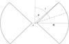 |
Fig. 9. Geometry used for the polarimetric simulation as outlined in the text. We note that i is the inclination angle, θ is the half opening angle, and r and R are the inner and outer radius of the outflow. |
Recently, many Monte Carlo codes have been developed which treat polarisation properties of Comptonisation (e.g. Schnittman & Krolik 2010; Tamborra et al. 2018; Zhang et al. 2019). For the Comptonising medium, these codes assume a pure electron cloud and, therefore, they are not adequate for the astrophysical situation we are studying. To our knowledge, the only other code which can, in principle, deal with the same problem is STOKES (Marin et al. 2018a,b; Goosmann & Gaskell 2007). However, the publicly available version of the code is tailored for IR-optical-UV radiation, rather than X-rays, so we decided to use the GHM94 code at this stage.
In the next two sub-sections, we present the cases of neutral and fully ionised matter, assuming unpolarised illuminating radiation. Then, we discuss the case of polarised primary radiation.
4.1. Neutral matter
We first discuss the results for neutral matter case. In Fig. 10a, the 2−10 keV polarisation degree as a function of the cosine of the inclination angle i of the system is shown for different values of NH, refl and θ. The primary spectrum, which is assumed to be unpolarised, is a power law with Γ = 2 in the energy range 2−30 keV. The emerging photons are then grouped in 20 angular bins, equally spaced in cos i. The polarisation is found to be always perpendicular to the symmetry axis of the system. For i lower than θ, the polarisation degree is low because of the dilution of the primary emission, which is unobstructed for those values. The polarisation degree is also low for small values of the equatorial column density because in those cases the matter is partially transparent, with consequent dilution by the primary radiation piercing through. This effect is also clear in Fig. 10c, where the dependence of the polarisation degree on the energy is shown as an illustration for an inclination angle of 65° (consistent with the one of GRS 1915+105), for four different θ values (30°, 45°, 60°, and 75°), three different NH, refl values (1, 3, and 5 × 1024 cm−2), and two different values of R (0.1 and 0.5).
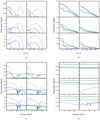 |
Fig. 10. Polarisation degree as a function of cosine of the inclination angle and energy. Panels a and c: refer to neutral matter, instead panels b and d: refer to ionised matter. In each of the plots, the left and the right represent R = 0.1 and 0.5, respectively. Top, middle, and bottom: represent NH, refl values of 1, 3, 5 × 1024 cm−2, respectively. The colours grey, blue, green, and black represent opening angles of 30°, 45°, 60°, and 75°, respectively. |
A strong decrease in the polarisation degree with energy is observed for low values of NH, refl, when the matter becomes transparent above a few kiloelectron volt. A much more constant polarisation degree is instead observed for high values of NH, refl when the matter is always optically thick. The two drops in the polarisation degree are due to the iron Kα and Kβ emission lines because fluorescent line emission is unpolarised.
4.2. Fully ionised matter
In the case of neutral matter, most of the reflected radiation is scattered once or a few times at most. When the matter is fully ionised, however, and if it is optically thick, photons can suffer many scatterings before escaping. As a result, the photon distribution is isotropic and the polarisation degree is much lower. This can be seen in Figs. 10b and d, which are the same as Figs. 10a and c, but in the fully ionised scenario. In this case, the polarisation degree is well below 10%, excluding the case for a θ of 75°, and almost energy-independent because at these energies the scattering cross section is still almost constant at the Thomson value. The modest increase in the polarisation degree for large optical depths is due to the fact that, because of Compton down-scattering, low energy photons emerging from the matter are scattered more times than high energy photons on average. The polarisation angle is again perpendicular to the symmetry axis of the system.
4.3. Polarised primary radiation
In the previous paragraphs, we calculated the polarisation of the radiation reflected by the outflow in the assumption of unpolarised primary radiation. However, if, as is widely believed, the primary radiation does indeed originate in a hot corona which Comptonises thermal radiation from the disc, a certain level of polarisation is expected, which depends on the geometry of the corona. For instance, Tamborra et al. (2018) explored two possible geometries for the corona, a slab covering the disc and a hemisphere centred on the black hole. The results depend on the coronal shape, the optical depth of the corona, and also the polarisation of the thermal disc emission (the latter was assumed to be either unpolarised or polarised following the Chandrasekhar formula, i.e. with a polarisation, parallel to the disc, ranging from zero for a disc viewed face-on to almost 12% for an edge-on view). Typically, the coronal polarisation ranges from zero (for emission perpendicular to the disc) to a maximum of 4% or so, with a polarisation degree either parallel or perpendicular to the disc axis (see e.g. Fig. 16 of Tamborra et al. 2018). To assess the effect of the polarisation of the primary emission – and in keeping in mind that the result for an arbitrary polarisation degree of the incident radiation can be obtained by properly combining the Stokes parameters of the reflected components arising from unpolarised and 100% polarised primary radiation – we simulated the response of the wind for a fully polarised primary radiation (independent of the direction of emission for simplicity), assuming a polarisation angle either perpendicular or parallel to the disc.
Polarisation of the reflected radiation results to be perpendicular to the disk axis and is independent of the polarisation angle of the primary radiation. It may be very high, reaching almost 80−90% in the case of perpendicular polarisation and neutral matter and/or small optical depths, when the reflection is dominated by photons scattered once, at least in the classical X-ray band. The degree of polarisation diminishes if the matter is ionised and the optical depth is large, because when photons undergo a high number of scatterings before escaping, the initial polarisation is largely forgotten. Indeed, for ionised matter and NH, refl = 1025 cm−2, the polarisation of the reflected radiation is only a few percent.
Because the polarisation angle of the reflected radiation is always the same, the total polarisation degree can be estimated for each energy and inclination angle with this simple formula: P ∼ PU * (1 − Pin)+PP * Pin, where PU and PP are the polarisation degrees of the reflected radiation illuminated by unpolarised and fully polarised primary emission, respectively, while Pin is the actual polarisation degree of the primary radiation (averaged over the emitting angle). Given that the last value is expected to be about 2−3% (Tamborra et al. 2018), even in the case of neutral matter and small optical depths (when PP is the highest), the polarisation degree of the reflecting matter may only be slightly higher than what have been calculated in the previous paragraphs. Given the uncertainties and limitation of our results discussed above, we decided to ignore the small effects of the polarisation of the primary radiation in the following.
4.4. The case of GRS 1915+105
We calculated the expected polarisation from the disc and the wind in the different flux levels estimated from Sect. 3. For the wind, we used the abovementioned scenarios (only from the side towards the line of sight), while for the case of disc we did a similar Monte-Carlo simulation for both neutral and fully ionised slab, isotropically illuminated by a point source from above (see Matt et al. 1989, 1991). The continuum emission coming from the corona is assumed to be unpolarised. In case of the disc, the polarisation angle is parallel to the symmetry axis of the system and perpendicular to the polarisation angle from the wind reflector. Figure 11 shows the inclination angle dependence of the polarisation degree in the case of the disc reflector. We also assumed a fully ionised state for log ξ which is greater than 2.5 and neutral for log ξ which is less than 2.5. Hence, in the case of the first flux level, we assume the disc to be neutral while the wind is fully ionised. In the other flux levels, both the disc and wind are fully ionised in these calculations. We used the absorbed flux in each energy bin to calculate the resulting polarisation degree. We did this calculation for different cases of opening angle, NH, refl, and R for the wind as outlined in the above sub-sections. The results of these calculations are given in Fig. 12. Since the polarisation from the disc and wind are perpendicular to each other, we assume the wind polarisation to be positive and the disc to be negative. We find that the highest polarisation degree (0.1 to 0.3) is when the opening angle of the wind is 75°. In the case of the first flux level, the wind dominates most of the spectra, while in the other flux levels the disc dominates beyond approximately 6 keV, at least for low values of the opening angle.
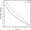 |
Fig. 11. Polarisation degree with respect to different inclination angles for the fully ionised and neutral scenario of a simple disc geometry. |
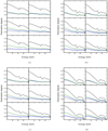 |
Fig. 12. Polarisation degree as a function of energy for GRS 1915+105 for different flux levels. Panels a–d: represent flux 1, flux 2, flux 3, and flux 4, respectively, as outlined in section 3. In each of the plots, the left and the right represent R = 0.1 and 0.5, respectively. Top, middle, and bottom: represent NH, refl values of 1, 3, 5 × 1024 cm−2, respectively. The colours grey, blue, green, and black represent opening angles of 30°, 45°, 60° and 75°, respectively. |
5. Discussion and conclusions
In this work, we explored how X-ray spectro-polarimetry can be used to constrain the geometrical parameters of the matter in the environment of the black hole in GRS 1915+105 in its present, obscured state. To do that, we first analysed three NuSTAR observations of GRS 1915+105 in the recent low flux state. Thanks to the wide hard X-ray energy band coverage of NuSTAR, we were able to constrain the continuum, which is heavily absorbed in the soft X-rays. NuSTAR observations indicate reflection-dominated spectra (see Sect. 4), suggesting that the central engine is still active and intrinsic absorption might be the reason for the observed low flux.
The main result of the spectral analysis is that the photon index is changing with respect to the change in flux. Hence the flares seen in the light curves are not merely due to a change in the absorption column density. The electron temperature shows an increase from the second to the last flux level, even though the trend seen is within a few kiloelectron volt.
Since the inclination angle is not constrained from spectroscopy alone, the change in the geometry of the reflector with respect to the flux will be an important perspective for the upcoming IXPE observations (Weisskopf et al. 2016). With the launch of IXPE late in 2021, the polarisation measurements in the low flux state of this source would be possible if the source remains in this state until then. X-ray polarimetry will not only assist to substantiate the spectral parameters, but it will also provide fundamental information regarding the geometry of the reflectors. A drop in the value of the polarisation degree at Fe Kα and Fe Kβ lines will indicate if the reflecting matter is neutral and hence the level of ionisation can be probed with polarimetry. From this work we see that the opening angle of the reflector can also be constrained from the polarisation degree. Moreover smaller values of R can give a higher polarisation, and hence the distance to the reflector can also be probed to an extent with polarimetry. However, in the OS, the continuum is highly absorbed in the 2−8 keV range and hence the properties of the inner disc and corona cannot be probed with polarimetry.
We simulated the expected IXPE observations using the simulation tool ixpeobssim (Pesce-Rollins et al. 2019) for the lowest and highest flux levels, and for two cases of the half opening angle (30° and 75°). For the simulation, we used the absorbed spectral model derived from the NuSTAR data in the 1−10 keV energy range. For the polarisation degree, we used the results from Sect. 4.4 for R = 0.1 and NH, refl = 1024 cm−2. For the polarisation angle, we assumed 90° and 0° for the wind and disc dominating energy ranges. The simulation results from all three detector units (DUs) were added in order to calculate the polarisation degree and angle in four energy bins for the two flux levels and the two opening angles. The results are shown in Fig. 13. This shows that with a 250 ks exposure of IXPE, we will be able to constrain the opening angle of the absorber and therefore provide the missing piece of the puzzle for GRS 1915+105.
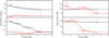 |
Fig. 13. Results of the IXPE simulations using ixpeobssim. The panel on the left refers to the polarisation degree, while the panel on the right refers to the polarisation angle. The top and bottom are for the lowest flux level and the highest flux levels, respectively. The red and black colours indicate a θ of 30° and 75°, respectively. |
Acknowledgments
We thank the anonymous referee for useful comments which helped us to significantly improve the paper. AR thanks Sudip Chakraborty, Riccardo Ferrazzoli and Keigo Fukumura for the useful comments and discussions. This research have made use of the archival data from the NASA’s High Energy Astrophysics Science Archive Research Center (HEASARC; https://heasarc.gsfc.nasa.gov/). We have also used the HEASoft software developed by HEASARC. The Italian contribution to the IXPE mission is supported by the Italian Space Agency (ASI) through the contract ASI-OHBI-2017-12-I.0, the agreements ASI-INAF-2017-12-H0 and ASI-INFN-2017.13-H0, and its Space Science Data Center (SSDC), and by the Istituto Nazionale di Astrofisica (INAF) and the Istituto Nazionale di Fisica Nucleare (INFN) in Italy.
References
- Arnaud, K. A. 1996, in Astronomical Data Analysis Software and Systems V, eds. G. H. Jacoby, & J. Barnes, ASP Conf. Ser., 101, 17 [NASA ADS] [Google Scholar]
- Balakrishnan, M., Miller, J. M., Reynolds, M. T., et al. 2021, ApJ, 909, 41 [NASA ADS] [CrossRef] [Google Scholar]
- Belloni, T., Klein-Wolt, M., Méndez, M., van der Klis, M., & van Paradijs, J. 2000, A&A, 355, 271 [Google Scholar]
- Boeer, M., Greiner, J., & Motch, C. 1996, A&A, 305, 835 [NASA ADS] [Google Scholar]
- Costa, E., Soffitta, P., Bellazzini, R., et al. 2001, Nature, 411, 662 [NASA ADS] [CrossRef] [Google Scholar]
- Dauser, T., García, J., Walton, D. J., et al. 2016, A&A, 590, A76 [NASA ADS] [CrossRef] [EDP Sciences] [Google Scholar]
- Dorman, B., Arnaud, K. A., & Gordon, C. A. 2003, AAS/High Energy Astrophysics Division, 7, 22.10 [NASA ADS] [Google Scholar]
- Fender, R. P., Garrington, S. T., McKay, D. J., et al. 1999, MNRAS, 304, 865 [Google Scholar]
- Fender, R. P., Belloni, T. M., & Gallo, E. 2004, MNRAS, 355, 1105 [NASA ADS] [CrossRef] [Google Scholar]
- Fukumura, K., Kazanas, D., Shrader, C., et al. 2017, Nat. Astron., 1, 0062 [NASA ADS] [CrossRef] [Google Scholar]
- Fukumura, K., Kazanas, D., Shrader, C., et al. 2018, ApJ, 864, L27 [NASA ADS] [CrossRef] [Google Scholar]
- Fukumura, K., Kazanas, D., Shrader, C., & Tombesi, F. 2020, Am. Astron. Soc. Meet. Abstr., 236, 208.01 [NASA ADS] [Google Scholar]
- García, J., & Kallman, T. R. 2010, ApJ, 718, 695 [CrossRef] [Google Scholar]
- García, J., Kallman, T. R., & Mushotzky, R. F. 2011, ApJ, 731, 131 [CrossRef] [Google Scholar]
- García, J., Dauser, T., Reynolds, C. S., et al. 2013, ApJ, 768, 146 [Google Scholar]
- Ghisellini, G., Haardt, F., & Matt, G. 1994, MNRAS, 267, 743 [Google Scholar]
- Goosmann, R. W., & Gaskell, C. M. 2007, A&A, 465, 129 [NASA ADS] [CrossRef] [EDP Sciences] [Google Scholar]
- Goosmann, R. W., & Matt, G. 2011, MNRAS, 415, 3119 [NASA ADS] [CrossRef] [Google Scholar]
- Iwakiri, W., Negoro, H., Kawai, N., et al. 2019, ATel, 12787, 1 [Google Scholar]
- Jithesh, V., Maqbool, B., Dewangan, G. C., & Misra, R. 2019, ATel, 12805, 1 [Google Scholar]
- Joye, W. A., & Mandel, E. 2003, in Astronomical Data Analysis Software and Systems XII, eds. H. E. Payne, R. I. Jedrzejewski, & R. N. Hook, ASP Conf. Ser., 295, 489 [NASA ADS] [Google Scholar]
- Kaper, L., Hammerschlag-Hensberge, G., & van Loon, J. T. 1993, A&A, 279, 485 [NASA ADS] [Google Scholar]
- Koljonen, K. I. I., & Tomsick, J. A. 2020, A&A, 639, A13 [EDP Sciences] [Google Scholar]
- Kong, L. D., Zhang, S., Chen, Y. P., et al. 2021, ApJ, 906, L2 [NASA ADS] [CrossRef] [Google Scholar]
- Krimm, H. A., Holland, S. T., Corbet, R. H. D., et al. 2013, ApJS, 209, 14 [NASA ADS] [CrossRef] [Google Scholar]
- Lee, J. C., Reynolds, C. S., Remillard, R., et al. 2002, ApJ, 567, 1102 [NASA ADS] [CrossRef] [Google Scholar]
- Marin, F., Dovčiak, M., & Kammoun, E. S. 2018a, MNRAS, 478, 950 [NASA ADS] [CrossRef] [Google Scholar]
- Marin, F., Dovčiak, M., Muleri, F., Kislat, F. F., & Krawczynski, H. S. 2018b, MNRAS, 473, 1286 [NASA ADS] [CrossRef] [Google Scholar]
- Matsuoka, M., Kawasaki, K., Ueno, S., et al. 2009, PASJ, 61, 999 [Google Scholar]
- Matt, G., Perola, G. C., Costa, E., & Piro, L. 1989, in Two Topics in X-Ray Astronomy, Volume 1: X Ray Binaries. Volume 2: AGN and the X Ray Background, eds. J. Hunt, & B. Battrick, ESA Spec. Publ., 296, 991 [NASA ADS] [Google Scholar]
- Matt, G., Perola, G. C., & Piro, L. 1991, A&A, 247, 25 [NASA ADS] [Google Scholar]
- Middleton, M. J., Walton, D. J., Alston, W., et al. 2021, MNRAS, 506, 1045 [NASA ADS] [CrossRef] [Google Scholar]
- Miller, L., Turner, T. J., Reeves, J. N., et al. 2006, A&A, 453, L13 [NASA ADS] [CrossRef] [EDP Sciences] [Google Scholar]
- Miller, J. M., Fabian, A. C., Kaastra, J., et al. 2015, ApJ, 814, 87 [NASA ADS] [CrossRef] [Google Scholar]
- Miller, J. M., Raymond, J., Fabian, A. C., et al. 2016, ApJ, 821, L9 [CrossRef] [Google Scholar]
- Miller, J. M., Zoghbi, A., Raymond, J., et al. 2020, ApJ, 904, 30 [Google Scholar]
- Motta, S. E., Kajava, J. J. E., Sánchez-Fernández, C., et al. 2017, MNRAS, 471, 1797 [NASA ADS] [CrossRef] [Google Scholar]
- Motta, S., Williams, D., Fender, R., et al. 2019, ATel, 12773, 1 [Google Scholar]
- NASA High Energy Astrophysics Science Archive Research Center (HEASARC) 2014, Astrophysics Source Code Library [record ascl:1408.004] [Google Scholar]
- Neilsen, J., & Lee, J. C. 2009, Nature, 458, 481 [NASA ADS] [CrossRef] [Google Scholar]
- Neilsen, J., Homan, J., Gendreau, K., et al. 2019, ATel, 12793, 1 [Google Scholar]
- Neilsen, J., Homan, J., Steiner, J. F., et al. 2020, ApJ, 902, 152 [Google Scholar]
- Oskinova, L. M., Feldmeier, A., & Kretschmar, P. 2012, MNRAS, 421, 2820 [NASA ADS] [CrossRef] [Google Scholar]
- Pesce-Rollins, M., Lalla, N. D., Omodei, N., & Baldini, L. 2019, Nucl. Instrum. Meth. Phys. Res. A, 936, 224 [Google Scholar]
- Ponti, G., Fender, R. P., Begelman, M. C., et al. 2012, MNRAS, 422, L11 [NASA ADS] [CrossRef] [Google Scholar]
- Ratheesh, A., Tombesi, F., Fukumura, K., et al. 2021, A&A, 646, A154 [NASA ADS] [CrossRef] [EDP Sciences] [Google Scholar]
- Reeves, J., Done, C., Pounds, K., et al. 2008, MNRAS, 385, L108 [Google Scholar]
- Reid, M. J., McClintock, J. E., Steiner, J. F., et al. 2014, ApJ, 796, 2 [Google Scholar]
- Schnittman, J. D., & Krolik, J. H. 2010, ApJ, 712, 908 [NASA ADS] [CrossRef] [Google Scholar]
- Tamborra, F., Matt, G., Bianchi, S., & Dovčiak, M. 2018, A&A, 619, A105 [NASA ADS] [CrossRef] [EDP Sciences] [Google Scholar]
- Trushkin, S. A., Nizhelskij, N. A., Tsybulev, P. G., Bursov, N. N., & Shevchenko, A. V. 2020, ATel, 13442, 1 [Google Scholar]
- Ueda, Y., Yamaoka, K., & Remillard, R. 2009, ApJ, 695, 888 [NASA ADS] [CrossRef] [Google Scholar]
- Vrtilek, S. D., & Boroson, B. S. 2013, MNRAS, 428, 3693 [NASA ADS] [CrossRef] [Google Scholar]
- Weisskopf, M. C., Ramsey, B., O’Dell, S., et al. 2016, in Space Telescopes and Instrumentation 2016: Ultraviolet to Gamma Ray, eds. J. W. A. den Herder, T. Takahashi, & M. Bautz, SPIE Conf. Ser., 9905, 990517 [NASA ADS] [CrossRef] [Google Scholar]
- Wilms, J., Allen, A., & McCray, R. 2000, ApJ, 542, 914 [Google Scholar]
- Zdziarski, A. A., Johnson, W. N., & Magdziarz, P. 1996, MNRAS, 283, 193 [NASA ADS] [CrossRef] [Google Scholar]
- Zdziarski, A. A., Segreto, A., & Pooley, G. G. 2016, MNRAS, 456, 775 [Google Scholar]
- Zhang, W., Dovčiak, M., & Bursa, M. 2019, ApJ, 875, 148 [NASA ADS] [CrossRef] [Google Scholar]
- Zoghbi, A., Miller, J. M., King, A. L., et al. 2016, ApJ, 833, 165 [NASA ADS] [CrossRef] [Google Scholar]
- Życki, P. T., Done, C., & Smith, D. A. 1999, MNRAS, 309, 561 [Google Scholar]
All Tables
All Figures
|
Fig. 1. Top: Swift/BAT and MAXI/GSC daily averaged light curves in energy range 15−50 keV and 2−20 keV, respectively. The red, blue, and black vertical lines denote the NuSTAR observations used in this work. The black dotted line roughly indicates the epoch at which the source enters the obscured state (OS). The flux is normalised to crab units. Bottom: evolution of hardness ratio (4−10 keV/2−4 keV) with time in MAXI/GSC. |
| In the text | |
|
Fig. 2. Hardness intensity diagram (HID) made using daily averaged MAXI/GSC light curves. The black and grey points indicate the data points before and after the transition epoch. The coloured points are during the MJD of the observations used in this work. |
| In the text | |
|
Fig. 3. NuSTAR/FPMA light curves in the 3−79 keV energy band. Top, middle, and bottom: represent obsID1, obsID2, and obsID3, respectively. The light curve is plotted from the start time of the observation and was binned at 10 s. |
| In the text | |
|
Fig. 4. Unfolded NuSTAR spectra of obsID1 (red), obsID2 (blue), obsID3 (black) modelled with the cutoffpl and galactic absorption for plotting purposes. The fitted models are shown by dotted lines in their respective colours. The plots shows only FPMA data. |
| In the text | |
|
Fig. 5. Geometry assumed for the best fit spectral model as outlined in the text. We note that 1, 2, and 3 represent reflection from the disc, continuum emission, and reflection from the wind, respectively. The continuum is assumed to originate from the corona above the black hole. The shaded portion indicates the disc wind, while the black horizontal structure represents the disc. |
| In the text | |
|
Fig. 6. Unfolded NuSTAR spectra for different flux levels as outlined in Sect. 3. The colours grey, blue, green, and black represent flux 1, flux 2, flux 3, and flux 4, respectively. The plots shows only FPMA data. |
| In the text | |
|
Fig. 7. Unabsorbed spectral components at different flux levels. Top: nthcomp. Middle: xillverCP2 – wind. Bottom: xillverCP1 – disc. The colours grey, blue, green, and black represent flux 1, flux 2, flux 3, and flux 4, respectively. |
| In the text | |
|
Fig. 8. Spectral parameters from the flux resolved spectroscopy with respect to the flux. The colours black, grey, blue, and green represent the spectral parameters of the continuum (nthcomp), ionised absorber (zxipcf), wind reflector (xillverCP1), and disc reflector (xillverCP2), respectively. Left: top, middle, and bottom: photon index, electron temperature, and NH of the ionised absorber, respectively. Right: top, middle, and bottom: ionisation parameter, red shift, and Rhard, respectively. |
| In the text | |
|
Fig. 9. Geometry used for the polarimetric simulation as outlined in the text. We note that i is the inclination angle, θ is the half opening angle, and r and R are the inner and outer radius of the outflow. |
| In the text | |
|
Fig. 10. Polarisation degree as a function of cosine of the inclination angle and energy. Panels a and c: refer to neutral matter, instead panels b and d: refer to ionised matter. In each of the plots, the left and the right represent R = 0.1 and 0.5, respectively. Top, middle, and bottom: represent NH, refl values of 1, 3, 5 × 1024 cm−2, respectively. The colours grey, blue, green, and black represent opening angles of 30°, 45°, 60°, and 75°, respectively. |
| In the text | |
|
Fig. 11. Polarisation degree with respect to different inclination angles for the fully ionised and neutral scenario of a simple disc geometry. |
| In the text | |
|
Fig. 12. Polarisation degree as a function of energy for GRS 1915+105 for different flux levels. Panels a–d: represent flux 1, flux 2, flux 3, and flux 4, respectively, as outlined in section 3. In each of the plots, the left and the right represent R = 0.1 and 0.5, respectively. Top, middle, and bottom: represent NH, refl values of 1, 3, 5 × 1024 cm−2, respectively. The colours grey, blue, green, and black represent opening angles of 30°, 45°, 60° and 75°, respectively. |
| In the text | |
|
Fig. 13. Results of the IXPE simulations using ixpeobssim. The panel on the left refers to the polarisation degree, while the panel on the right refers to the polarisation angle. The top and bottom are for the lowest flux level and the highest flux levels, respectively. The red and black colours indicate a θ of 30° and 75°, respectively. |
| In the text | |
Current usage metrics show cumulative count of Article Views (full-text article views including HTML views, PDF and ePub downloads, according to the available data) and Abstracts Views on Vision4Press platform.
Data correspond to usage on the plateform after 2015. The current usage metrics is available 48-96 hours after online publication and is updated daily on week days.
Initial download of the metrics may take a while.