© H. M. Schmid 2021

1 Introduction

Circumstellar disks reflect the light from the central star, and the produced scattered intensity and polarization contain a lot of information about the disk geometry and the scattering dust particles. The scattered light of disks is usually only a contribution of a few percent or less to the direct light from the central star and therefore requires observations with sufficiently high resolution and contrast to resolve the disk from the star. This was achieved in recent years for many circumstellar disks with adaptive optics (AO) systems at large telescopes using polarimetry, a powerful high-contrast technique, to disentangle the scattered and therefore polarized light of the disk from the direct and typically unpolarized light of the central star (e.g., Apai et al. 2004; Oppenheimer et al. 2008; Quanz et al. 2011; Hashimoto et al. 2011; Muto et al. 2012).

With AO systems, the observational point spread function (PSF) depends to a large extent on the atmospheric turbulence and is highly variable (e.g., Cantalloube et al. 2019). For this reason, the disks are often only detected in polarized light and it is not possible to disentangle the disk intensity signal from the strong, variable PSF of the central star (see e.g., Esposito et al. 2020). Therefore, analyses of the scattered light from the disk are often based on the differential polarization alone and only in favorable cases can one combine this with measurements of the disk intensity. For the data analysis, the observed polarization must first be corrected for instrumental polarization effects, and this is relatively difficult for complex AO systems (e.g., Schmid 2021, and references therein). For this reason, the first generation of AO systems with polarimetric mode provided useful qualitative polarimetric results but hardly any quantitative results.

This situation has changed with the new extreme AO systems GPI (Macintosh et al. 2014) and SPHERE (Beuzit et al. 2019), which, in addition to better image quality, also provide polarimetrically calibrated data for the circumstellar disk (Perrin et al. 2015; Schmid et al. 2018; de Boer et al. 2020; van Holstein et al. 2020). Thus, quantitative polarization measurements are now possible for many circumstellar disks. However, the technique is not yet well established, and detailed studies haveonly been made for a few bright, extended disks; for example for HR 4796A (Perrin et al. 2015; Milli et al. 2019; Arriaga et al. 2020), HIP 79977 (Engler et al. 2017), HD 34700A (Monnier et al. 2019), HD 169142 (Tschudi & Schmid 2021), and HD 142527 (Hunziker et al. 2021). There also exist a few polarimetric studies based on HST polarimetry, such as those for the disks of AU Mic (Graham et al. 2007) or AB Aur (Perrin et al. 2009). The large majority of polarimetric disk observations in the literature focus their analysis on the high-resolution disk geometry (e.g., Benisty et al. 2015; Garufi et al. 2016; Avenhaus et al. 2018), and therefore the measurements are not calibrated and polarimetric cancelation effects introduced by the limited spatial resolution are not taken into account. Even for the detailed polarimetric studies mentioned above, the derived photo-polarimetric parameters are relatively heterogeneous. Convolution effects are only sometimes taken into account, and measurements are given as observed maps, azimuthal or radial profiles, or as dust parameters of a well-fitting disk model. This makes a comparison of results between different studies difficult and inaccurate, in particular because measuring uncertainties and model ambiguities are rarely discussed in detail.

Therefore, this paper introduces Stokes Q and U quadrant polarization parameters, which are simple to derive but still well defined, and facilitate systematic, quantitative studies of larger samples of circumstellar disks in order to make polarimetric measurements more valuable for our understanding of the physical properties of the scattering dust. Quantitative polarimetry of disks might be very useful to clarify whether dust properties are different or similar for systems with different morphology, age, level of illumination, or dust composition. The quadrant polarization parameters should also be useful for model simulations describing the appearance of a given disk for different inclinations so that intrinsic properties can be disentangled from the effects of a particular disk inclination. The same parameters can also be used to quantify the impact of the convolution of the intrinsic disk signal or of simulated images with instrumental PSF profiles to correct the observable polarization of small and large disks for the effects of smearing and polarimetric degradation (Schmid et al. 2006).

Using Stokes Q and U quadrant parameters for the description of the polarization of disks is a new approach and to the best of our knowledge this is the first publication using this type of analysis. These quadrant polarization parameters are introduced in Sect. 2 using the published data of Milli et al. (2019) for the bright debris disk HR 4796A as an example. The interpretation of the measured values is illustrated with corresponding model calculations for optically thin debris disks, which are described in Sect. 3. The models are similar to the classical simulation for the scattered intensity of debris disks of Artymowicz et al. (1989) and Kalas & Jewitt (1996), but they also consider the scattering polarization as in the models of Graham et al. (2007) and Engler et al. (2017). It is shown in Sect. 4 that the relative quadrant polarization values for optically thin, axisymmetric (and flat) debris disks are independent of the radial dust distribution and they depend only on the disk inclination i and the shape of the polarized scattering phase function f_ϕ(θ). Therefore, in Sect. 5 we construct simple diagnostic diagrams for quadrant polarization parameters which constrain the f_ϕ (θ) function for a given i, or directly yield the scattering asymmetry parameter g if we adopt a Henyey-Greenstein scattering function for the dust. The diagnostic diagrams are applied to the quadrant polarization measurements of HR 4796A and the obtained results are compared with the detailed, model-free phase-curve extraction of Milli et al. (2019). Finally, in Sect. 6 we discuss the potential and limitations of the quadrant polarization parameters for the analysis of disk observations and model simulations in a broader context.

2 Quadrant polarization parameters for disks

2.1 Polarization parameters in sky coordinates

Polarimetric imaging of stellar systems with circumstellar disks provides typically sky images for the intensity I_obs (α, δ) and the Stokes linear polarization parameters Q_obs(α, δ) and U_obs(α, δ). For dust scattering, the circular polarization is expected to be much smaller than the linear polarization and is usually not measured; it is therefore neglected in this work. Q and U are differential quantities for the linear polarization components $$Q=I_0-I_{90}\text{and}U=I_{45}-I_{135},$$(1)

which can also be expressed as polarization flux 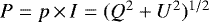$P=p\times I={(Q^2+U^2)}^{1/2}$ and polarization position angle θ_P = 0.5 atan2(U, Q)¹. The polarized flux p × I is by definition a positive quantity, which, for noisy Q or U imaging data, suffers from a significant bias effect (Simmons & Stewart 1985).

The azimuthal Stokes parameter Q_ϕ can be used as an alternative for P for circumstellar disks. Q_ϕ measures polarization in the azimuthal direction with respect to the central star (α₀, δ₀) and U_ϕ in a direction rotated by 45° with respect to azimuthal. Circumstellar dust, which scatters light from the central star, mostly produces polarization with azimuthal orientations θ_P ≈ ϕ_αδ + 90°, while U_ϕ is almost zero. Therefore, Q_ϕ can be considered as a good approximation for the polarized flux of the scattered radiation from circumstellar disks 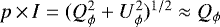$p\times I={(Q_{\varphi }^2+U_{\varphi }^2)}^{1/2}\approx Q_{\varphi }$, and this approximation also avoids the noise bias problem (Schmid et al. 2006). For the model calculations of optically thin disks presented in this work, there is strictly p × I = Q_ϕ, while small signals U_ϕ < 0.05 Q_ϕ can be produced by multiple scattering in optically thick disks (Canovas et al. 2015) or disks with aligned aspherical scattering particles. The U_ϕ signal is often much larger, that is, U_ϕ ≳ 0.1 Q_ϕ, in observations because of the PSF convolution problem for poorly resolved disks and polarimetric calibration errors. Both effects should be taken into account and corrected for the polarimetric measurements of disks. The azimuthal Stokes parameters are defined by $$Q_{\varphi }(\alpha ,\delta )=-Q(\alpha ,\delta )\cos (2{\varphi }_{\alpha \delta })-U(\alpha ,\delta )\sin (2{\varphi }_{\alpha \delta }),$$(2) $$U_{\varphi }(\alpha ,\delta )=+Q(\alpha ,\delta )\sin (2{\varphi }_{\alpha \delta })-U(\alpha ,\delta )\cos (2{\varphi }_{\alpha \delta }),$$(3)

with $${\varphi }_{\alpha \delta }=\text{atan2}((\delta -{\delta }_0),(\alpha -{\alpha }_0)),$$(4)

according to the description of Schmid et al. (2006) for the radial Stokes parameters Q_r, U_r, and using Q_ϕ = −Q_r and U_ϕ = −U_r.

2.2 Disk integrated polarization parameters

Quantitative measurements of the scattered radiation from circumstellar disks were obtained in the past with aperture polarimetry, which provided the disk-integrated Stokes parameters $\overline{Q}$, $\overline{U}$ or the polarized flux 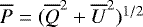$\overline{P}={({\overline{Q}}^2+{\overline{U}}^2)}^{1/2}$ usually expressed as fractional polarization relative to the system-integrated intensity $\overline{Q}/{\overline{I}}_{\text{tot}}$, $\overline{U}/{\overline{I}}_{\text{tot}}$, or $\overline{P}/{\overline{I}}_{\text{tot}}$ and the averaged polarization position angle 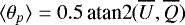$\langle {\theta }_p\rangle =0.5\text{atan2}(\overline{U},\overline{Q})$ (e.g., Bastien 1982; Yudin & Evans 1998). This polarization signal can be attributed to the scattered light from the disk if the star produces no polarization and if the interstellar polarization can be neglected, or if these contributions can be corrected. Usually, the disk intensity 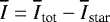$\overline{I}={\overline{I}}_{\text{tot}}-{\overline{I}}_{\text{star}}$ cannot be distinguished from the stellar intensity with aperture polarimetry, apart from a few exceptional cases, such as that of β Pic.

Aperture polarimetry provides only the net scattering polarization, but misses potentially strong positive and negative polarization components + Q, −Q and + U, −U which cancel each other in unresolved observations. Therefore, $\overline{Q}$ and $\overline{U}$, or $\overline{P}$ and ⟨θ_p⟩ provide onlyone value and one direction for circumstellar disks, which agglomerate all possible types of deviations from axisymmetry of the scattering polarization of a circumstellar disk.

Disk-resolved polarimetric imaging avoids or strongly reduces the destructive cancellation effect and provides therefore much more information about the scattering polarization of disks. The most basic polarization parameter for the characterization of a resolved disk is the disk integrated azimuthal polarization ${\overline{Q}}_{\varphi }$ which can be considered as equivalent to the polarized flux for resolved observations $\overline{P}$². The integrated polarized flux ${\overline{Q}}_{\varphi }$ depends on the spatial resolution of the data; this aspect is not considered in this work because for well-resolved disks, like that of HR 4796A, the effect of limited spatial resolution is small and can be corrected with modeling of the instrumental smearing.

If the disk intensity $\overline{I}$ is measurable, one can also determine the disk-averaged fractional polarization 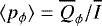$\langle p_{\varphi }\rangle ={\overline{Q}}_{\varphi }/\overline{I}$. Unfortunately, it is still often very difficult to measure the disk intensity I(α, δ) with AO-observations because the signal cannot be separated from the intensity of the variable point spread function I_star (α, δ) of the much brighter central star. In these cases, the fractional polarization can only be expressed relative to the total system intensity $\langle p_{\varphi ,\text{tot}}\rangle ={\overline{Q}}_{\varphi }/{\overline{I}}_{\text{tot}}$. Integrated or averaged quantities are well defined but not well suited to characterizing the polarimetric features and the azimuthal dependence of the polarization for circumstellar disks. Therefore, we introduce new polarization parameters to quantify the individual positive and negative polarimetric components + Q, − Q and + U, − U of spatially resolved disk observations and models.

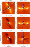Fig. 1 Illustration of the definition of the quadrant polarization parameters (panels e and f) for the observations of the debris disk around HR 4796A from Milli et al. (2019). Left: Azimuthal polarization Qϕ and Stokes Q and U in relative α, δ-sky coordinates. Right: Qϕ, Qd, and Ud in x, y-disk coordinates.

2.3 Quadrant polarization parameters in disk coordinates

For polarimetric imaging of circumstellar disks, the geometric orientation of the disk and the Stokes Q and U parameters are often described in sky coordinates. This is inconvenient for the characterization of the intrinsicscattering geometry of the disk and therefore we define new polarization parameters Q_d and U_d in the disk coordinate system (x, y), where the central star is at x₀ = 0, y₀ = 0 and the x and y are aligned with the major and minor axis of the projected disk, respectively. The positive x-axis is pointing left to ease the comparison with observations in relative sky coordinates α − α₀ and δ − δ₀ and to get the same convention for the Q_d and U_d orientations in x, y and sky images. Thus, the relative α − α₀, δ − δ₀ sky coordinates of the observed images I, Q_ϕ, Q, and U must be rotated according to $$x=(\alpha -{\alpha }_0)\cos \omega +(\delta -{\delta }_0)\sin \omega ,$$(5) $$y=(\delta -{\delta }_0)\cos \omega -(\alpha -{\alpha }_0)\sin \omega .$$(6)

as shown in Fig. 1 for the imaging polarimetry of HR 4796A using ω = 242° (− 118°). We use the convention that ω aligns the more distant semi-minor axis of the projected disk with the positive (upward) y-axis.

Also, the Stokes parameters for the linear polarization must be rotated from the Q, U sky system to the Q_d, U_d disk system using the geometrically rotated (x, y)-frames $$Q_{\text{d}}(x,y)=Q(x,y)\cos (2\omega )+U(x,y)\sin (2\omega ),$$(7) $$U_{\text{d}}(x,y)=U(x,y)\cos (2\omega )-Q(x,y)\sin (2\omega ).$$(8)

We define for the Q_d(x, y) and U_d(x, y) polarization images the quadrant parameters Q₀₀₀, Q₀₉₀, Q₁₈₀, and Q₂₇₀ for Stokes Q_d and U₀₄₅, U₁₃₅, U₂₂₅, and U₃₁₅ for Stokes U_d, which are obtained by integrating the Stokes Q_d or U_d disk polarization signal in the corresponding quadrants as shown in Figs. 1e and f. This selection of polarization parameters is of course motivated by the natural Q and U quadrant patterns for circumstellar scattering where the signal in a given quadrant typically has the same sign everywhere and is almost zero at the borders of the defined integration region. This is strictly the case for all the model calculations for optically thin debris disks presented in this work and the same type of quadrant pattern is also predominant for the scattering polarization of proto-planetary disks. Multiple scattering and grain alignment effects can introduce deviations from a “clean” quadrant polarization pattern which may be measurable in high-quality observations (Canovas et al. 2015). However, the smearing and polarization cancellation effects introduced by the limited spatial resolution are typically much more important in affecting the quadrant pattern. For poor spatial resolution or very small disks, the quadrant pattern disappears (Schmid et al. 2006) or is strongly disturbed for asymmetric systems (Heikamp & Keller 2019).

Eight quadrant polarization values seems to be a useful number for the characterization of the azimuthal distribution of the polarization signal of disks. The parameters provide some redundancy to check and verify systematic effects, or to allow alternative disk characterizations if one parameter is not easily measurable or is affected by a special disk feature. Let us consider the redundancy in the context of the geometrical symmetry of disks and the dust scattering asymmetry.

For an inclined, but intrinsically axisymmetric disk, the Stokes Q_d quadrants have the symmetry $$Q_{090}=Q_{270,}$$(9)

and the Stokes U_d quadrants have the anti-symmetries $$U_{045}=-U_{315}\text{and}{U}_{135}=-U_{225}.$$(10)

Special cases generate additional equalities; for example the models with isotropic scattering (see Fig. 5) have a front–back symmetry and therefore there is also Q₀₀₀ = Q₁₈₀ and U₀₄₅ = −U₁₃₅ = U₂₂₅ = −U₃₁₅. For an axisymmetric disk seen pole-on, all quadrant parameters have the same absolute value. If a disk deviates from an intrinsically symmetric geometry, for example a brighter + x side, then this would result in |Q₀₉₀| > |Q₂₇₀| for Stokes Q_d and |U₀₄₅| > |U₃₁₅| or |U₁₃₅| > |U₂₂₅| for Stokes U_d.

Dust, which is predominantly forward scattering, produces more signal for front side polarization quadrants compared to the backside quadrants and this is equivalent to |Q₁₈₀| > |Q₀₀₀| or |U₁₃₅| > |U₀₄₅| and |U₂₂₅| > |U₃₁₅|. Properties that can be deduced from parameter ratios derived from the same data set are important because this reduces the impact of at least some systematic uncertainties in the measurements.

The quadrant parameters are also linked to the integrated polarization parameters ${\overline{Q}}_{\varphi }$, ${\overline{Q}}_{\text{d}}$, and ${\overline{U}}_{\text{d}}$. For the sum of all four Stokes Q_d and Stokes U_d quadrants, there is $$\Sigma Q_{xxx}={\overline{Q}}_{\text{d}}\text{and}\Sigma U_{xxx}={\overline{U}}_{\text{d}}.$$(11)

For pole-on systems, there is 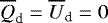${\overline{Q}}_{\text{d}}={\overline{U}}_{\text{d}}=0$, because of the symmetric cancellation of positive and negative quadrants and intrinsically axis-symmetric systems have ${\overline{U}}_{\text{d}}=0$ for all disk inclinations because of the left–right antisymmetry. Axisymmetric but inclined systems have ${\overline{Q}}_{\text{d}}\ne 0$ in general. For disks with larger inclination i, a smaller fraction of the disk is “located” in the quadrants Q₀₀₀ and Q₁₈₀ and a larger fraction is located in Q₀₉₀ and Q₂₇₀ near the major axis because of the disk projection. Edge-on disks are almost only located in the quadrants Q₀₉₀ and Q₂₇₀ and quadrant sums approach Q₀₀₀ + Q₁₈₀ → 0 and 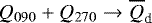$Q_{090}+Q_{270}\to {\overline{Q}}_{\text{d}}$ for i → 90°.

For the sums of the four absolute quadrant parameters for Stokes Q_d, there is of course $$\Sigma \left|Q_{xxx}\right|>\Sigma Q_{xxx}\text{and}\Sigma \left|Q_{xxx}\right|<{\overline{Q}}_{\varphi },$$(12)

and the equivalent exists for sums of the Stokes U_d quadrants. For a pole-on view, the system is axisymmetric with respect to the line of sight and there is 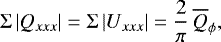$$\Sigma \left|Q_{xxx}\right|=\Sigma \left|U_{xxx}\right|=\frac{2}{\pi }{\overline{Q}}_{\varphi },$$(13)

where each quadrant has the same absolute value of 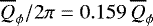${\overline{Q}}_{\varphi }/2\pi =0.159{\overline{Q}}_{\varphi }$. These sums will converge for edge-on disks i = 90° to $\Sigma \left|Q_{xxx}\right|\to {\overline{Q}}_{\varphi }$ for Stokes Q_d and to Σ |U_xxx|→ 0 for Stokes U_d.

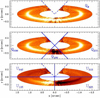Fig. 2 Apertures used for the measurements of the integrated azimuthal polarization ${\overline{Q}}_{\varphi }$ (top), the Stokes Qd quadrants (middle), and the Stokes Ud quadrants (bottom) for HR 4796A.

2.4 Quadrant polarization parameters for HR 4796A

We use the high-quality differential polarimetric imaging (DPI) of the bright debris disk HR 4796A from Milli et al. (2019) shown in Fig. 1 as an example for the measurement of the quadrant polarization parameters. The data were taken with the SPHERE/ZIMPOL instrument (Beuzit et al. 2019; Schmid et al. 2018) in the very broad band (VBB) filter with the central wavelength λ_c = 735 nm and full width of Δλ = 290 nm.

These data provide “only” the differential Stokes Q(x, y) and U(x, y) signals or the corresponding azimuthal quantities Q_ϕ(x, y) and U_ϕ(x, y), but no intensity signal because it is difficult with AO-observations to separate the disk intensity from the variable intensity PSF of the much brighter central star. The scattered light of the disk around HR 4796A was previously detected in polarization and intensity with AO systems in the near-IR (e.g., Milli et al. 2017; Chen et al. 2020; Arriaga et al. 2020), and in intensity in the visual with HST (e.g., Schneider et al. 2009).

Quadrant polarization parameters Q_xxx and U_xxx for HR 4796A derived from the data shown in Figs. 1e and f are given in Table 1 as relative values using the integrated polarized flux ${\overline{Q}}_{\varphi }$ as reference.The quadrant values were obtained by integrating the counts in the annular apertures sections as illustrated in Fig. 2, which avoid the high noise regions from the PSF peak in the center. The uncertainties indicated in Table 1 account for the image noise, but do not account for systematic effects related to the selected aperture geometry or polarimetric calibration uncertainties. The noise errors are particularly large for the quadrants Q₀₀₀ and Q₁₈₀ because of the small separation of these disk sections from the bright star and additional negative noise spikes which are particularly strong for the Q₀₀₀ quadrant. Because of this noise, the formal integration gives $Q_{000}/{\overline{Q}}_{\varphi }=-0.04$. From the decreasing trend of the signal in for example Q_ϕ towards theback side of the disk and the measured disk signals of about 0.03 for $U_{045}/{\overline{Q}}_{\varphi }$ or $U_{315}/{\overline{Q}}_{\varphi }$, an absolute signal of less than $\left|Q_{000}\right|/{\overline{Q}}_{\varphi }<0.01$ is expected fora smooth dust distribution in the ring and any reasonable assumptions for the dust scattering. Therefore, we do not consider the noisy Q₀₀₀-measurement in the quadrant sums ΣQ_xxx. The noise in the Q₁₈₀-quadrant is also significantly enhanced when compared to other quadrants despite the relatively strong signal and the small integration area. A detailed analysis of the noise pattern might improve the measuring accuracy, but this is beyond the scope of this paper.

Because of the noise, the apertures for Q_ϕ and the quadrants U₀₄₅ and U₁₃₅ were restricted to avoid the noisy and essentially signal-free region around ϕ_xy ≈ 0°. One should note that uncertainties for the quadrant measurements, for example for Q₁₈₀, also affect the Q_ϕ value and a dominant noise feature therefore has an enhanced impact on relative parameters such as $Q_{xxx}/{\overline{Q}}_{\varphi }$, which include the disk integrated azimuthal polarization ${\overline{Q}}_{\varphi }$. These are typical problems for high-contrast observations of inclined disks and it can be very useful to select only high-signal-to-noise quadrant values for the characterization of the azimuthal dependence of the disk polarization.

Asymmetries between the left and right or the positive and negative sides of the x-axis can be deduced from the absolute quadrant parameters |Q₀₉₀| and |Q₂₇₀|, |U₀₄₅| and |U₃₁₅|, and |U₁₃₅| and |U₂₂₅|. Table 1 gives relative left–right brightness differences ${\Delta }_{bbb}^{aaa}$ calculated according to $${\Delta }_{270}^{090}=\frac{\left|Q_{090}\right|-\left|Q_{270}\right|}{\left|Q_{090}\right|+\left|Q_{270}\right|}$$(14)

for Stokes Q_d parameters and equivalent for ${\Delta }_{315}^{045}$ and ${\Delta }_{225}^{135}$ for Stokes U_d.

The asymmetry values ${\Delta }_{270}^{090}$ and ${\Delta }_{225}^{135}$ both yield more flux on the left side of the (x, y)-plane, which is the SW-side for the HR 4796A disk. This does not agree with previous determinations, including even the analysis of the same data by Milli et al. (2019) who measured more flux on the NE side. A more detailed investigation reveals that the peak surface brightness is indeed higher for the disk on the NE side and that the left–right asymmetry depends on the width of the annular apertures used for the flux extraction. If we integrate only a narrow annular region with a full width of Δx = 0.1″ at the location of the major axis then we also get more flux for the NE side or negative ${\Delta }_{270}^{090}$-values of − 3 ± 2% but still less than the “negative” (SW-NE) asymmetry measured by Milli et al. (2019) for Q_ϕ or Schneider et al. (2018) for the intensity. We therefore conclude that there are subtle asymmetries at the level of Δ ≈ 10% present for the disk HR 4796A, which are positive for a wide flux extraction and negative for a narrow flux extraction. Measurement uncertainties in the left–right differences are at the few percent level for bright quadrant pairs.

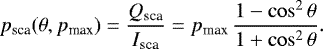
The back-side to front-side brightness contrast can be expressed with quadrant ratios such as $${\Lambda }_{180}^{000}=\frac{\left|Q_{000}\right|}{\left|Q_{180}\right|},\text{and}\text{}{\Lambda }_{135}^{045}=\frac{\left|U_{045}\right|}{\left|Q_{135}\right|},\text{or}{\Lambda }_{225}^{315}=\frac{\left|U_{315}\right|}{\left|U_{225}\right|},$$(15)

and their equivalents for other quadrant ratios. These ratios are small ≲ 0.5 for HR 4796A which is indicative of dust with a strong forward scattering phase function. For isotropic scattering in an axisymmetric disk, the ratios would be ${\Lambda }_{180}^{000}={\Lambda }_{135}^{045}=1$ for all inclinations. Because the polarization flux in the backside quadrants is small, one can also assess the disk forward scattering with a comparison of the brighter Q₀₉₀ and Q₂₇₀ quadrants with the Stokes Q_d front quadrant Q₁₈₀ or the Stokes U_d front quadrants U₁₃₅ and U₂₂₅ as given in Table 1.

As demonstrated in Table 1, the polarization quadrants provide a useful set of parameters for the quantitativecharacterization of the geometric distribution of the polarization signal in circumstellar disks. Comparisons with model calculations are required to assess the diagnostic power of the derived values for the determination of the scattering properties of the dust or for the interpretation of the strength of disk asymmetries.

3 Disk model calculations

The simple disk models presented in this work follow the basic calculations for the scattered intensity from debris disks (Artymowicz et al. 1989; Kalas & Jewitt 1996) and the scattering polarization (e.g., Bastien & Menard 1988; Whitney & Hartmann 1992; Graham et al. 2007; Engler et al. 2017) but focus on the azimuthal dependence of the scattering polarization and the determination of the quadrant polarization values. The model disks are described by a dust-density distribution in cylindrical coordinates ρ(r, φ_d, h) where r is the radius vector $r={(x_{\text{d}}^2+y_{\text{d}}^2)}^{-1/2}$ and φ_d the azimuthal angle in the disk plane³, where x_d coincides with x for the major axis of the projected, inclined disk. We consider in this work very simple, optically thin τ ≪ 1, axisymmetric models ρ(r, h), where the dust scattering cross-section per unit mass σ_sca is independent of the location. The total dust scattering emissivity (integrated over all directions) ϵ(r, h) of a volume element is given by the stellar flux F_λ(r, h) = L_λ∕(4π(r² + h²)), the disk density ρ(r, h), and σ_sca: $$ϵ(r,h)=\frac{L_{\lambda }}{4\pi (r^2+h^2)}\rho (r,h){\sigma }_{\text{sca}}.$$(16)

The incident flux decreases as F_λ ∝ 1∕R² with R² = r² + h², because in our optically thin scattering model we neglect the extinction of stellar light by the dust and the addition of diffuse light produced by the scatterings in the disk.

The resulting images for the scattered light intensity I(x, y) and the azimuthal polarization Q_ϕ(x, y) are obtained with a line of sight or z-axis integration of the scattering emissivity ϵ and the scattering phase functions f_I(θ_xyz, g) for the intensity $$I(x,y)={\displaystyle \int ϵ}(x,y,z)f_I({\theta }_{xyz},g)\text{d}z,$$(17)

and f_ϕ(θ_xyz, g, p_max) for the polarized intensity $$Q_{\varphi }(x,y)={\displaystyle \int ϵ}(x,y,z)f_{\varphi }({\theta }_{xyz},g,p_{\text{max}})\text{d}z.$$(18)

The transformations from the disk coordinate system (r, φ_d, h) with x_d = rsinφ_d and y_d = rcosφ_d to the sky coordinate system (x, y, z) is given by x = x_d, y = y_d cosi + hsini and z = y_d sini − hcosi where i is the disk inclination. This also defines the scattering angle θ_xyz and the radial separation to the central star R_xyz for each point (x, y, z).

3.1 Scattering phase functions

The scattering phase function f_I(θ, g) for the intensity is described by the Henyey-Greenstein function or HG-function (Henyey & Greenstein 1941), where θ is the angle of deflection $$f_I(\theta ,g)=\frac{1}{4\pi }\frac{1-g^2}{{(1+g^2-2g\cos \theta )}^{3/2}}.$$(19)

The asymmetry parameter g is defined between − 1 and + 1 and backward scattering dominates for negative g, forward scattering dominates for positive g, while the scattering is isotropic for g = 0.

The scattering phase function f_ϕ(θ, g, p_max) for the polarized flux adopts the same angle dependence for the fractional polarization as Rayleigh scattering, but with the scale factor p_max ≤ 1 for the maximum polarization at θ = 90°. This description is often used (e.g., Graham et al. 2007; Buenzli & Schmid 2009; Engler et al. 2017) as a simple approximation for a Rayleigh scattering-like angle dependence but reduced polarization induced by dust particles (e.g., Kolokolova & Kimura 2010; Min et al. 2016; Tazaki et al. 2019).

The angle dependence of the fractional polarization of the scattered light is $$p_{\text{sca}}(\theta ,p_{\text{max}})=\frac{Q_{\text{sca}}}{I_{\text{sca}}}=p_{\text{max}}\frac{1-{\cos }^2\theta }{1+{\cos }^2\theta }.$$(20)

The scattered intensity I_sca can be split into the perpendicular I_⊥ and parallel I_∥ polarization components with respect to the scattering plane, so that I_sca = I_⊥ + I_∥, Q_sca = I_⊥− I_∥ and I_⊥ = (I_sca + Q_sca)∕2, I_∥ = (I_sca − Q_sca)∕2. Together with p_sca, this yields $$I_{\perp }(p_{\text{max}},\theta )=I_{\text{sca}}\cdot [0.5+p_{\text{max}}(\frac{1}{1+{\cos }^2\theta }-0.5)],$$(21) $$I_{\parallel }(p_{\text{max}},\theta )=I_{\text{sca}}\cdot [0.5+p_{\text{max}}(\frac{{\cos }^2\theta }{1+{\cos }^2\theta }-0.5)],$$(22)

or, expressed as scattering phase functions, f_⊥ = f_I k_⊥ (θ, p_max) and f_∥ = f_I k_∥ (θ, p_max), where k_⊥ and k_∥ are the expressions in the square brackets and p_sca = k_⊥− k_∥.

The scattering plane in a projected image of a circumstellar disk has always a radial orientation with respect to the central star. Therefore the induced scattering polarization Q_sca, which is perpendicular to the scattering plane, translates into an azimuthal polarization Q_ϕ for the projected disk map. The scattering phase functions are related by $$f_{\varphi }(\theta ,g,p_{\text{max}})=p_{\text{max}}{f}_{\varphi }^n(\theta ,g)=f_I(\theta ,g)p_{\text{sca}}(\theta ,p_{\text{max}}),$$(23)

where f_ϕ can be separated into a normalized part $f_{\varphi }^n$ for p_max = 1 and the scale factor p_max.

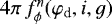
Figure 3 illustrates the scattering phase functions for g = 0.2 for the total intensity f_I and the corresponding polarization components f_⊥ and f_∥ for p_max = 0.5 and 0.2. The differential phase function f_ϕ = f_⊥− f_∥ has the same θ-dependence $f_{\varphi }^n(\theta ,g)$ for both cases, and only the amplitude scales with p_max. In this formalism, the total intensity phase function f_I(g, θ) does not depend on the adopted polarization parameter p_max. Expected values for approximating dust scattering with HG scattering functions are p_max ≈ 0.05−0.8, but we often set this scale factor in this work to p_max = 1 because this allows us to plot the intensity and polarization on the same scale. A value p_max = 1 applies for Rayleigh scattering but the HG-function with g = 0 (isotropic scattering) differs from the Rayleigh scattering function for the intensity⁴. 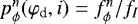Hereafter, f_ϕ (θ, g, p_max) and $f_{\varphi }^n(\theta ,g)$ are also referred to as the HG_pol-function and normalized HG_pol-function, respectively.

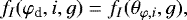
The polarimetric scattering phase function for the azimuthal Stokes parameters f_ϕ can be converted into phase functions f_Q and f_U for the Stokes Q_d and U_d parameters $$f_Q({\theta }_{xyz},g,p_{\text{max}})=-f_{\varphi }({\theta }_{xyz},g,p_{\text{max}})\cos (2{\varphi }_{xy}),$$(24) $$f_U({\theta }_{xyz},g,p_{\text{max}})=-f_{\varphi }({\theta }_{xyz},g,p_{\text{max}})\sin (2{\varphi }_{xy}),$$(25)

where ϕ_xy = atan2(y, x) is the azimuthal angle in the sky coordinates aligned with the disk as illustrated in Fig. 1. These simple relations are valid in our optical thin (single scattering) models because U_ϕ (x, y) = 0 and the Stokes Q_d(x, y) and U_d (x, y) model images can then be calculated as in Q_ϕ in Eq. (18) but using the phase functions for f_Q and f_U.

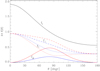Fig. 3 Scattering phase functions for the HG asymmetry parameter g = 0.2 for the total intensity 4π fI(θ) (black), for the polarized intensities 4π f⊥(θ) (dashed) and 4π f∥(θ) (dotted), for the two values pmax = 0.5 (red) and 0.2 (blue), and the corresponding scattering phase functions for the polarized flux 4π fϕ (θ) (full, colored lines).

3.2 Flat disk models and azimuthal phase functions

The calculations for the scattered flux I(x, y) and polarization Q_ϕ(x, y) with Eqs. (17) and (18) are strongly simplified for a flat disk because the integrations for a given x-y coordinate along the z-coordinate can be replaced by single values for the separation r_xy from the star, for the scattering emissivity ϵ(r_xy), and for the scattering angle θ_xy. The volume density ρ must be replaced by a vertical surface density Σ(r) or a line-of-sight surface density Σ(r)∕cosi. Of course, the scattering in the disk plane must still be treated as in an optically thin disk, $$\tau (r)={\displaystyle {\int }_0^r{\kappa }_{\Sigma }}\Sigma (r)\text{d}r\ll 1,$$(26)

where κ_Σ = a_Σ + σ_Σ is the disk extinction coefficient composed of the contributions from absorption a_Σ and scattering σ_Σ.

3.2.1 Projected flat disk image

The scattered intensity and polarization for a flat disk are given by $$I(x,y)=ϵ(r_{xy})f_I({\theta }_{xy},g),$$(27) $$Q_{\varphi }(x,y)=ϵ(r_{xy})f_{\varphi }({\theta }_{xy},g,p_{\text{max}}),$$(28)

and similar for the Stokes Q_d(x, y) and U_d(x, y) using the phase function from Eqs. (24) and (25). The scattering emissivity $$ϵ(r_{xy})=\frac{L_{\lambda }}{4\pi r_{xy}^2}{\sigma }_{\Sigma }\frac{\Sigma (r_{xy})}{\cos i}$$(29)

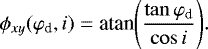
is proportional to the line-of-sight surface density Σ(r_xy)∕cos i, which considers the disk inclination, and where $r_{xy}^2=x^2+{(y/\cos i)}^2$ and θ_xy = acos(−z_xy∕r_xy) = acos(−ytani∕r_xy), because y = y_d cosi and z_xy = y_d sini.

In these equations for I(x, y), Q_ϕ (x, y), Q_d (x, y), and U_d (x, y), the radial dependence of the scattering emissivity ϵ(r_xy) is separatedfrom the azimuthal dependence described by the scattering phase functions f_I (θ_xy), f_ϕ (θ_xy), f_Q (θ_xy), and f_U (θ_xy). This is very favorable forthe introduced quadrant parameters, which describe the polarization of the scattered light of disks with an azimuthal splitting of the signalQ_d(x, y) → Q₀₀₀, Q₀₉₀, Q₁₈₀, Q₂₇₀ and U_d(x, y) → U₀₄₅, U₁₃₅, U₂₂₅, U₃₁₅ by integrating the polarization in the corresponding quadrants outlined by the black lines in the Q_d and U_d panels of Figs. 4 and 5.

Disk images for I(x, y), Q_d (x, y), U_d (x, y), and Q_ϕ (x, y) for flat diskmodels are shown in Fig. 4 for the asymmetry parameter g = 0.3, the scale factor p_max = 1, and three different inclinations i = 0°, 45°, and 75°. For the radial surface scattering emissivity, a radial dependence ϵ(r) ∝ 1∕r is adopted extending from an inner radius r₁ to the outer radius r₂ = 2 r₁. Along the x-axis, the scattering angle is always θ_xy = 90° and the surface brightness increases for higher inclinations as in the inclined surface emissivity ∝ 1∕cosi.

The scattering asymmetry parameter g is relatively small and therefore the front–back brightness differences are not strong in Fig. 4. The forward scattering effect is much clearer in Fig. 5, where two disks are plotted with the same i and ϵ(r), but for isotropic scattering g = 0 and strong forward scattering g = 0.6.

For the disks shown in Figs. 4 and 5, the absolute signal drops in the radial direction for all azimuthal angles ϕ_xy = atan2(x, y) by exactly a factor of two from the inner edge ${(r_1)}_{xy}$ to the outer edge ${(r_2)}_{xy}$ according to the adopted radial dependence of the scattering emissivity ϵ(r)∝ 1∕r. This is equivalent to the statement that the (relative) azimuthal dependence along the ellipse r_xy describing aring in the inclined disk is the same for all separations in a given disk image I(r_xy, φ_d), Q_ϕ (r_xy, φ_d), Q_d (r_xy, φ_d), or U_d (r_xy, φ_d). This is also valid if the azimuthal angle φ_d for the disk plane is replaced by the on-sky azimuthal angle ϕ.

Therefore, it is possible to determine the azimuthal dependence of the scattered light in a very simple way using azimuthal phase functions defined in the disk plane, without considering the radial distribution of the scattering emissivity.

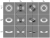Fig. 4 I-, Qd -, Ud - and Qϕ -images for a flat disk with g = 0.3, pmax = 1, and for inclinations i = 0°, i = 45°, and 75°. The same gray scale from + a (white) to −a (black) is used for all panels. The black lines in the Qd and Ud panels indicate the polarization quadrants.

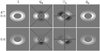Fig. 5 I-, Qd -, Ud - and Qϕ -images for flat disks with i = 45°, pmax = 1, and for scattering asymmetry parameter g = 0.0 and 0.6. The same gray scale from + a (white) to −a (black) is used for all panels.

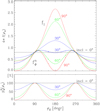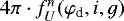
Fig. 6 Upper panel: azimuthal dependence of the disk scattering phase function for the intensity 4π fI (φd, i, g) and the normalized (pmax = 1) polarized intensity $4\pi f_{\varphi }^n({\phi }_{\text{d}},i,g)$ for disks with scattering asymmetry parameter g = 0.3 and inclinations i = 0°,  30°,  60°, and 90°. Lower panel:normalized fractional polarization $p_{\varphi }^n({\phi }_{\text{d}},i)=f_{\varphi }^n/f_I$ for the same inclinations; $p_{\varphi }^n$ does not depend on the g-parameters.

3.2.2 Scattering phase functions for the disk azimuth angle

The azimuthal dependence of the scattered light can be calculated easily for flat, rotationally symmetric, and optically thin disks as a function of the azimuthal angle φ_d in the disk plane. For this, we have to express the scattering angle θ as a function of φ_d and the diskinclination i according to $${\theta }_{\phi ,i}=\theta ({\phi }_{\text{d}},i)=\text{acos}(\cos {\phi }_{\text{d}}\cdot (-\sin i)),$$(30)

where φ_d = 0 for the far-side semi-minor axis of the projected disk.

The dependence of the scattered intensity and polarization flux with disk azimuthal angle φ_d follows directly from the scattering phase functions f_I and f_ϕ and the change of the scattering angle θ as a function of φ_d and i $$f_I({\phi }_{\text{d}},i,g)=f_I({\theta }_{\phi ,i},g),$$(31) $$f_{\varphi }({\phi }_{\text{d}},i,g,p_{\text{max}})=p_{\text{max}}{f}_{\varphi }^n({\theta }_{\phi ,i},g)=f_{\varphi }({\theta }_{\phi ,i},g,p_{\text{max}}).$$(32)

Figure 6 shows the azimuthal scattering functions 4π f_I(φ_d, i, g) for the intensity and $4\pi f_{\varphi }^n({\phi }_{\text{d}},i,g)$ for the polarized flux for g = 0.3 and for different inclinations. The factor 4π normalizes the isotropic scattering case 4π f_I(φ_d, i, g = 0) = 1 and scales all other cases g≠0 accordingly.

The enhanced forward scattering for f_I(φ_d) around φ_d = 180° is clearly visible for inclined disks. The polarization function $f_{\varphi }^n({\phi }_{\text{d}})$ has for backward scattering around φ_d = 0° and forward scattering around φ_d = 180° strongly reduced values in highly inclined disks when compared to the intensity as can be seen for the green and red curves in Fig. 6. At φ_d = 90° and 270°, the functions f_I and $f_{\varphi }^n$ have (for given g) the same value for all inclinations because the scattering angles are always θ_φ,i = 90° (cos φ_d = 0 in Eq. (30)).

The azimuthal dependence of the fractional polarization is given by $$p_{\varphi }^n({\phi }_{\text{d}},i)=\frac{p_{\text{sca}}({\theta }_{\phi ,i})}{p_{\text{max}}}=\frac{f_{\varphi }^n({\phi }_{\text{d}},i,g)}{f_I({\phi }_{\text{d}},i,g)},$$(33)

and this function does not depend on the asymmetry parameter g. This dependence is equivalent to Rayleigh scattering and is shown in Fig. 6 for completeness.

For the phase function f_Q and f_U one needs to consider that the Stokes Q_d and U_d parameters are defined in the disk coordinate system projected onto the sky while f_ϕ is given for the azimuthal angle φ_d for the x_d, y_d-coordinates of the disk midplane. For the splitting of f_ϕ(φ_d, i, g, p_max) into f_Q and f_U, the azimuthal angle ϕ_xy defined in the x-y sky plane must be used. The relation between φ_d and ϕ_xy is $${\varphi }_{xy}({\phi }_{\text{d}},i)=\text{atan}(\frac{\tan {\phi }_{\text{d}}}{\cos i}).$$(34)

The phase functions for Q_d and U_d are then equivalent to the conversion given in Eqs. (24) and (25): $$f_Q({\phi }_{\text{d}},i,g,p_{\text{max}})=-f_{\varphi }({\phi }_{\text{d}},i,g,p_{\text{max}})\cdot \cos (2{\varphi }_{xy}({\phi }_{\text{d}},i))$$(35) $$f_U({\phi }_{\text{d}},i,g,p_{\text{max}})=-f_{\varphi }({\phi }_{\text{d}},i,g,p_{\text{max}})\cdot \sin (2{\varphi }_{xy}({\phi }_{\text{d}},i)).$$(36)

These azimuthal function of the “on-sky” Stokes parameters f_Q and f_U is shown in Fig. 7. The functions are characterized by their double wave, which for i = 0° are exact double-wave cosine f_Q(φ_d) ∝−cos2φ_d and double-wavesine f_U(φ_d) ∝−sin2φ_d functions. Deviations from the sine and cosine function become larger with increasing i, particularly for large asymmetry parameters g. The positive and negative sections of the f_Q(φ_d) and f_U(φ_d) functions correspond to the positive and negative polarimetric quadrants. The f_Q and f_U functions can also be expressed as normalized functions $f_Q^n$ and $f_U^n$ for p_max = 1 and as fractional polarization $p_Q^n$ and $p_U^n$ equivalent to $p_{\varphi }^n$ given above.

For the adopted HG_pol dust scattering phase function, these phase functions f_φ provide a universal description of the azimuthal flux and polarized flux dependence as a function of inclination i for all flat, optically thin, rotationally symmetric disks.

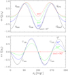Fig. 7 Azimuthal dependence for the Stokes scattering phase functions $4\pi \cdot f_Q^n({\phi }_{\text{d}},i,g)$ and $4\pi \cdot f_U^n({\phi }_{\text{d}},i,g)$ for a rotationally symmetric, flat, optically thin disk with scattering asymmetry parameter g = 0.3 and inclinations i = 0°,  30°,  60°, and 90°.

3.2.3 Disk-averaged scattering functions

The total intensity $\overline{I}$ for our disk model can be conveniently calculated in r, φ_d-coordinates because the integration can be separated between the r-dependent scattering emissivity ϵ and the φ_d-dependent scattering phase function f_I according to $$\overline{I}=2\pi {\displaystyle {\int }_0^{\infty }ϵ}(r)r\text{d}r\cdot \frac{1}{2\pi }{\displaystyle {\int }_0^{2\pi }{f}_I}({\phi }_{\text{d}},i,g)\text{d}\phi =\overline{ϵ}\cdot \langle f_I(i,g)\rangle .$$(37)

The first term represents the total scattering emissivity $\overline{ϵ}$ of the disk, and the second term is the disk averaged scattering phase function for the intensity ⟨f_I (i, g)⟩.

For the integrated polarization parameters, the same type of relation can be used $${\overline{Q}}_{\varphi }=\overline{ϵ}\cdot \langle f_{\varphi }(i,g,p_{\text{max}})\rangle ,$$(38) $${\overline{Q}}_{\text{d}}=\overline{ϵ}\cdot \langle f_Q(i,g,p_{\text{max}})\rangle ,$$(39) $${\overline{U}}_{\text{d}}=\overline{ϵ}\cdot \langle f_U(i,g,p_{\text{max}})\rangle .$$(40)

The scale factor p_max can be separated from the normalized versions of the disk-averaged scattering functions as $$\langle f_{\varphi }(i,g,p_{\text{max}})\rangle =p_{\text{max}}\langle f_{\varphi }^n(i,g)\rangle ,$$(41)

and similar for f_Q and f_U. The disk-averaged fractional polarization follows from $$\langle p_{\varphi }(i,g,p_{\text{max}})\rangle =p_{\text{max}}\langle p_{\varphi }^n(i,g)\rangle =\frac{\langle f_{\varphi }(i,g,p_{\text{max}})\rangle }{\langle f_I(i,g)\rangle },$$(42)

and similar for p_Q or p_U, where the latter is always zero for rotationally symmetric disks. Unlike for the azimuthal dependence of the fractional polarization pⁿ (φ_d, g), the disk-averaged parameters $\langle p_{\varphi }^n(i,g)\rangle$ depend on the g-parameter because in this average g shifts the flux weight between disk regions producing higher or lower levels of scattering polarization.

3.3 Normalized quadrant polarization parameters

The Stokes Q_xxx and U_xxx quadrant polarization parameters correspond to the individual positive and negative sections of the f_Q (φ_d) and f_U (φ_d) disk phase function shown in Fig. 7. The relation between quadrant parameters and phase function follow the same scheme as for the disk-integrated quantities ${\overline{Q}}_{\text{d}}$ and ${\overline{U}}_{\text{d}}$ described by Eq. (37) but the integration is limited to the azimuthal angle range φ₁ to φ₂ of a given quadrant instead of 0 to 2π. For Stokes Q_d, there is $$Q_{xxx}=({\phi }_2-{\phi }_1){\displaystyle {\int }_0^{\infty }ϵ}(r)r\text{d}r\cdot \frac{p_{\text{max}}}{{\phi }_2-{\phi }_1}{\displaystyle {\int }_{\phi 1}^{\phi 2}{f}_Q^n}({\phi }_{\text{d}},i,g)\text{d}\phi .$$(43)

The first term is the disk scattering emissivity ϵ integrated for the quadrant and the second term is the averaged $f_Q^n$ scattering phase function for this quadrant. Because ϵ is independent of the azimuthal angle, the first term can be expressed as a fraction of the disk integrated emissivity $\overline{ϵ}\cdot ({\phi }_2-{\phi }_1)/2\pi$ and the equation takes the form 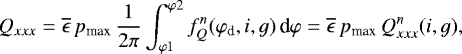$$Q_{xxx}=\overline{ϵ}{p}_{\text{max}}\frac{1}{2\pi }{\displaystyle {\int }_{\phi 1}^{\phi 2}{f}_Q^n}({\phi }_{\text{d}},i,g)\text{d}\phi =\overline{ϵ}{p}_{\text{max}}{Q}_{xxx}^n(i,g),$$(44)

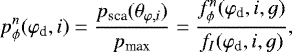
where we introduce the normalized quadrant polarization $Q_{xxx}^n$. The same scaling factors $\overline{ϵ}$ and p_max are involved as for the equations for the integrated polarization parameters ${\overline{Q}}_{\varphi }$, ${\overline{Q}}_{\text{d}}$, and ${\overline{U}}_{\text{d}}$, and therefore $Q_{xxx}^n$ and ⟨f_Q (i, g)⟩ are related with the same factors $\overline{ϵ}$ and p_max to observed quantities Q_xxx and ${\overline{Q}}_{\text{d}}$. The same formalism applies to the Stokes U_d quadrants.

According to Eq. (44), the normalized polarization quadrants $Q_{000}^n$, $Q_{090}^n$, $Q_{180}^n$, $Q_{270}^n$ and $U_{045}^n$, $U_{135}^n$, $U_{225}^n$, $U_{315}^n$ depend only on i and g as in the disk-averaged functions $\langle f_Q^n\rangle$ or $\langle f_U^n\rangle$. The azimuthal integration range φ₁ to φ₂ is of course different for each quadrant, as summarized in Table 2. For the Q_d -quadrants, the geometric projection effect introduces an inclination dependence for the integration boundaries φ₁ and φ₂. For increased i, the fraction of the sampled disk surfaces s_xxx = (φ₁(i) − φ₂(i))∕2π in the left and right quadrants $Q_{090}^n$ and $Q_{270}^n$ is enhanced s₀₉₀ = s₂₇₀ = 0.5 −atan(cosi)∕π and the disk surface fraction located in the front and back quadrants $Q_{180}^n$ and $Q_{000}^n$ is reduced s₀₀₀ = s₁₈₀ = atan(cosi)∕π, respectively (we note that atan(cos0°) = π∕4 and atan(cos90°) = 0). There is no i-dependence for the splitting of the Stokes U_d quadrants, because the “left-side” back and front quadrants and the “right-side” back and front quadrants sample the same disk surface fraction s₀₄₅ = s₁₃₅ = s₂₂₅ = s₃₁₅ = 0.25 for all inclinations.

4 Calculation of disk polarization parameters

The previous section shows that the disk-integrated radiation parameters such as $\overline{I},{\overline{Q}}_{\varphi }$ and the quadrant polarization parameters Q_xxx and U_xxx can be expressed as disk-averaged phase functions ⟨f(i, g)⟩ and normalized polarization parameters $Q_{xxx}^n(i,g)$ and $U_{xxx}^n(i,g)$ describing the azimuthal dependence of the scattering, and scale factors for the total disk-scattering emissivity $\overline{ϵ}$ and the maximum scattering polarization p_max.

This simplicity allows a concise but comprehensive graphical presentation covering the full parameter space of the disk model parameters for the intensity and polarization, including the newly introduced quadrant polarization parameters. The Appendix gives a few IDL code lines for calculation of the numerical values. In addition, we explore the deviation of the results from vertically extended disk models and from the flat disk models.

Fig. 8 Disk-averaged scattering phase functions for the intensity 4π ⟨fI⟩, the normalized (pmax=1) azimuthal polarization $4\pi \langle f_{\varphi }^n\rangle$, and the normalized Stokes Qd flux $4\pi \langle f_Q^n\rangle$ versus the disk inclination for HG-asymmetry parameters g = 0 (black), 0.3 (blue), 0.6 (red), and 0.9 (green). Lines give the results for flat disks and crosses for vertically extended disk rings (Sect. 4.3, Fig. 11).

4.1 Calculations of the disk-averaged intensity and polarization scattering functions

The disk-averaged scattering phase functions ⟨f(i, g)⟩ are equivalent to the basic integrated quantities $\overline{I}$, ${\overline{Q}}_{\varphi }$, and ${\overline{Q}}_{\text{d}}$ if normalized scale factors $\overline{ϵ}=1$ and p_max = 1 are used (Eqs. (37) to (39)). The functions ⟨f_I(i, g)⟩, $\langle f_{\varphi }^n(i,g)\rangle ,$ and $\langle f_Q^n(i,g)\rangle$ are plotted in Fig. 8 as a function of inclination for the four asymmetry parameters g = 0, 0.3, 0.6, and 0.9. The plot includes the results from calculation of vertically extended, three-dimensional disk rings (crosses) for comparison, which are discussed in Sect. 4.3. The results for ⟨f(i, g)⟩ are multiplied by the factor 4π because this sets the special reference case for isotropically scattering dust g = 0 for all inclinations to $4\pi \langle f_I(i,0)\rangle =4\pi \langle f_{\varphi }^n(i,0)\rangle =1$ and simplifies the discussion.

For pole-on disks i = 0°, there is $\langle f_{\varphi }^n(0^{°},g)\rangle =\langle f_I(0^{°},g)\rangle$ for all g parameters because the scattering angle is θ = 90° everywhere. For enhanced scattering asymmetry parameters g > 0 (but also for g < 0), the disk intensity is below the isotropic case 4π⟨f_I⟩ < 1 for lesser and moderately inclined disks i ≲ 60°, because theenhanced forward scattering (or backward scattering) produces enhanced scattered flux in directions near to the disk plane and reduced flux for polar viewing angles.

The forward scattering enhances the scattered intensity to 4π⟨f_I⟩ > 1 for i≳60° and this effect becomes particularly strong for g → 1 and i → 90°. This behavior is well known and produces a strong detection bias for high-inclination debris disks (e.g., Artymowicz et al. 1989; Kalas & Jewitt 1996; Esposito et al. 2020).

For the polarized flux $\langle f_{\varphi }^n(i,g)\rangle ,$ an enhanced inclination does not produce an enhancement of the ⟨f_ϕ ⟩ signal because the strong increase in scattered flux from the forward scattering direction (or backward direction for g < 1) is predominantly unpolarized. For moderate asymmetry parameter |g| ≲ 0.6, this causes an overall decrease of ⟨f_ϕ ⟩ with inclination (Fig. 8) while for extreme values |g|≳ 0.9 the huge flux increase compensates for the lower fractional polarization for forward and backward scattering.

The phase function for the Stokes Q_d parameter $\langle f_Q^n(0^{°},g)\rangle$ is zero for the pole-on view because of the symmetric cancellation of + Q_d and − Q_d signals. The function increases steadily with i (Fig. 8) and for i = 90° or edge-on disks there is $\langle f_Q^n({90}^{°},g)\rangle =\langle f_{\varphi }^n({90}^{°},g)\rangle$, because all dust is aligned with the major axis and produces polarization in the + Q_d direction.

Fractional polarization

The fractional polarizations $\langle p_{\varphi }^n(i,g)\rangle$ and $\langle p_Q^n(i,g)\rangle$ in Fig. 9 can be deduced from the ratio of the phase functions shown in Fig. 8. Observationally, a fractional polarization determination requires a measurement of the integrated disk polarization and the integrated disk intensity.

As shown in Fig. 9, the fractional azimuthal polarization $\langle p_{\varphi }^n(i,g)\rangle$ only depends to a very small extent on g for small inclinations i ≤ 35° with deviations <± 0.02 and the i-dependence is well described by $$\frac{{\overline{Q}}_{\varphi }}{\overline{I}}=p_{\text{max}}\langle p_{\varphi }^n(i)\rangle \approx p_{\text{max}}\cdot {(\cos i)}^{1.7}.$$(45)

A measurement of the fractional azimuthal polarization for low-inclination disks is therefore equivalent to a determination of the p_max-parameter.

The lower panel of Fig. 9 includes also the purely polarimetric ratio $\langle p_Q\rangle /\langle p_{\varphi }\rangle ={\overline{Q}}_{\text{d}}/{\overline{Q}}_{\varphi }$, which includes no scaling factor p_max and systematic uncertainties from the polarimetric measurements might be particularly small. Therefore, the ratio ${\overline{Q}}_{\text{d}}/{\overline{Q}}_{\varphi }$ can be used to determine the scattering asymmetry parameter g, if polarimetric cancellation effects for ${\overline{Q}}_{\varphi }$ are taken into account for poorly resolved disks. 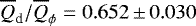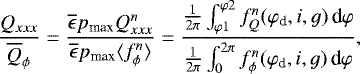For the extended disk HR 4796A, cancellation can be neglected, and we can use ${\overline{Q}}_{\text{d}}/{\overline{Q}}_{\varphi }=0.652\pm 0.030$ ($\Sigma Q_{xxx}/{\overline{Q}}_{\varphi }$ from Table 1) and the inclination i = 75°, which yields a value of about g = 0.7 from Fig. 9. This method is useful for systems with i ≈ 30°−80° because the separations between the g-parameter curves are quite large. The curves in Fig. 9 for flat disk models are not applicable for edge-on disks i≳80° with a vertical extension (see Sect. 4.3).

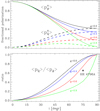Fig. 9 Upper panel: disk averages of the fractional azimuthal polarization $\langle p_{\varphi }^n\rangle$ and the Stokes Qd polarization $\langle p_Q^n\rangle$ normalized for pmax = 1 for different asymmetry parameters and as function of inclination. Lower panel: polarization ratios $\langle p_Q\rangle /\langle p_{\varphi }\rangle ={\overline{Q}}_{\text{d}}/{\overline{Q}}_{\varphi }$ and the corresponding measurement for HR 4796A.

4.2 Calculations of the normalized quadrant polarization parameters

The normalized quadrant polarization parameters $Q_{000}^n$, $Q_{090}^n$, $Q_{180}^n$, and $U_{045}^n$ $U_{135}^n$ are plotted in Fig. 10 as a function of i for different g parameters. The “right-side” quadrants $Q_{270}^n$, $U_{315}^n$, $U_{225}^n$ have the same absolute values as the corresponding “left-side” quadrants because of the disk symmetry. All values are multiplied by the factor 2π so that the reference case g = 0 and i = 0° is set to $2\pi |Q_{xxx}^n(0^{°},0)|=2\pi |U_{xxx}^n(0^{°},0)|=1,$ similar to the normalization for the disk-averaged scattering function $4\pi \langle f_{\varphi }^n(i,0)\rangle$.

For pole-on disks, all the normalized quadrant polarization values have the same absolute value $|Q_{xxx}^n(0^{°},g)|=|U_{xxx}^n(0^{°},g)|$ for a given g. This value is lower for larger g-parameter because lesslight is scattered perpendicularly to the disk plane in the polar direction, as in the $\langle f_{\varphi }^n\rangle$ function. For i > 0° the quadrant values show different types of dependencies on i and g.

As described in Sect. 3.3, for the Stokes Q_d quadrants the disk inclination introduces a geometric projection effect which increases the sampled disk area for the “left” and “right” quadrants for larger i, and therefore the $Q_{090}^n$ and $Q_{270}^n$-values reach a maximum of ($Q_{\varphi }^n/2$) for i = 90°. The areas for the front and back quadrants go to zero for i → 90° and therefore so do the values $Q_{180}^n$ and $Q_{000}^n$, but with a difference which depends strongly on g. The effect of the scattering asymmetry is already clearly visible for relatively small values, g ≈ 0.3, and inclinations, i ≈ 10°, and becomes even stronger for larger g and i as can be seen from the enhanced |Q₁₈₀| values relative to |Q₀₀₀|. A similar front–back quadrant effect also occurs for the U_d-components with enhanced absolute values for the front-side quadrant |U₁₃₅| and reduced values for the backside quadrant |U₀₄₅|.

4.3 Comparison with three-dimensional disk ring models

The polarization parameters derived in the previous sections are calculated for geometrically flat disks because this simplifies the calculations enormously. Of course, real disks have a vertical extension but observations of highly inclined debris disks typically show a small ratio h∕r≲0.1 (see e.g., Thébault 2009). Therefore, the flat disk models could serve as an approximation for 3D disks, and we explore the differences. For this, we calculated models for a rotationally symmetric, optically thin disk ring with a central radius r_ring and a Gaussian density distribution for the ring cross-section, $$\rho (r,h)={\rho }_0\text{exp}(-[{(r-r_{\text{ring}})}^2+h^2]/2{\delta }^2),$$(46)

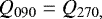
with full width at half maximum (FWHM) of Δ_FWHM = 2.355 δ. Figure 11 compares images of such 3D disk rings with Δ_FWHM = 0.2 r_ring, g = 0.6, and different i with flat disk models. The vertical extension of the 3D model is most obvious for the edge-on (i =90°) case for which the flat disk model gives only a profile along the x-axis.

For i < 90°, the differences between flat disks and vertically extended disks are already small for i = 75° and hardly recognizable for lower inclination. In particular, the values for the disk-averaged scattering functions ⟨f⟩ and the normalized quadrant polarization parameters $Q_{xxx}^n$ and $U_{xxx}^n$ are equal or very similar as can be seen in Figs. 8 and 10 where the results from the 3D disks are plotted as small crosses together with those from the flat disk models. The agreement is typically better than ± 0.01. An example of a systematic difference between 3D disks and flat disks is a slightly lower value (about 0.01) for the azimuthal polarization ⟨f_ϕ ⟩ in Fig. 8 for pole-on (i = 0°) 3D disks. For disks with a vertical extension, not all scatterings are occurring exactly in the disk midplane, but also slightly above and below where the scattering angle is smaller or larger than 90° and therefore (1 − cos²θ)∕(1 + cos²θ) in Eq. (20) is smaller than one. Another example is the reduced ⟨f_I ⟩ for edge-on (i = 90°) 3D disks, because less material lies exactly in front of the star where forward scattering would produce a strong maximum for large g-parameter. This is most visible for g = 0.6 (the effect is even stronger for g = 0.9 but this point is outside the plotted range). Similar but typically also very small effects are visible for the normalized quadrant polarization parameters in Fig. 10. The presence or absence of the vertical extension produces a strong difference for the Stokes U_d which is also clearly apparent in Fig. 11 for i = 90°.

These comparisons show that the quadrant polarization parameters derived from flat, optically thin, rotationally symmetric disk models are for most cases essentially indistinguishable from those derived from 3D disk models with a vertical extension typical for debris disks. Only for edge-on or close to edge-on disks, i≳80°, can the vertical extension introduce significant differences, which needs to be taken into account.

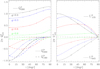Fig. 10 Normalized ($p_{\text{max}}=1,\overline{ϵ}=1$) quadrant polarization parameters for $2\pi Q_{000}^n$, $2\pi Q_{090}^n$, $2\pi Q_{180}^n$ (left) and $2\pi U_{045}^n$, $2\pi U_{135}^n$ (right) as function of disk inclination and for the HG-asymmetry parameter g = 0 (black), 0.3 (blue), 0.6 (red), and 0.9 (green). Lines give the results for flat disks and crosses for vertically extended disk rings (Sect. 4.3, Fig. 11).

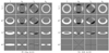Fig. 11 Comparison of the 3D-ring model with the flat disk model. Left: I, Qd, Ud and Qϕ for a 3D disk ring with a full width at half maximum density distribution of ΔFWHM∕rring = 0.2. Scattering parameters are g = 0.6 and pmax = 1 for inclinations i = 0°, 45°, 75° and 90°. The same gray scale from + a (white) to −a (black) is used for all panels. The black lines in the Qd and Ud panels indicate the polarization quadrants. Right: same but for the flat disk model.

5 Diagnostic diagrams for the scattering asymmetry g

The normalized quadrant polarization parameters and quadrant ratios for disk models using the HG_pol-function depend only on the scattering asymmetry parameter g and the diskinclination i as shown in Fig. 10. From imaging polarimetry of debris disks one can often accurately measure the disk inclination, and therefore the quadrant polarization parameters are ideal for the determination of g. The method described in this work for the single parameter HG_pol-function can be generalized to other, more sophisticated parameterizations for the polarized scattering phase function of the dust.

This diagnostic method is based on the strong assumption that the intrinsic disk geometry is rotationally symmetric, which is often a relatively good assumption for debris disks, but there are also several cases known with significant deviations from axisymmetry (e.g., Debes et al. 2009; Maness et al. 2009; Hughes et al. 2018). This can affect the determination of the g-parameter and one should always assess possible asymmetries in the disk symmetry using for example the left–right symmetry parameters ${\Delta }_{270}^{090}$ or ${\Delta }_{225}^{135}$ (Sect. 2.4).

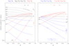Fig. 12 Relative quadrant polarization values $\left|Q_{000}\right|/{\overline{Q}}_{\varphi }$ (blue), $\left|Q_{090}\right|/{\overline{Q}}_{\varphi }$ (black) $\left|Q_{180}\right|/{\overline{Q}}_{\varphi }$ (red) on the left and $\left|U_{045}\right|/{\overline{Q}}_{\varphi }$ (blue), $\left|U_{135}\right|/{\overline{Q}}_{\varphi }$ (red) on the right for flat disk models with different i and as a function of the scattering asymmetry parameter g. The measured values for HR 4796A are given on the right side in each panel and the corresponding g-parameter is given at the top or bottom using the i = 75°curves for these derivations.

5.1 Relative quadrant parameters

The azimuthal dependence of the scattering polarization can be described by the relative quadrant parameters $Q_{xxx}/{\overline{Q}}_{\varphi }$ and $U_{xxx}/{\overline{Q}}_{\varphi }$. These parameters are directly linked to the normalized scattering phase functions $f_Q^n$, $f_U^n$, and $f_{\varphi }^n$ for the polarization according to $$\frac{Q_{xxx}}{{\overline{Q}}_{\varphi }}=\frac{\overline{ϵ}{p}_{\text{max}}{Q}_{xxx}^n}{\overline{ϵ}{p}_{\text{max}}\langle f_{\varphi }^n\rangle }=\frac{\frac{1}{2\pi }{\displaystyle {\int }_{\phi 1}^{\phi 2}{f}_Q^n}({\phi }_{\text{d}},i,g)\text{d}\phi }{\frac{1}{2\pi }{\displaystyle {\int }_0^{2\pi }{f}_{\varphi }^n}({\phi }_{\text{d}},i,g)\text{d}\phi },$$(47)

and equivalent to $U_{xxx}/{\overline{Q}}_{\varphi }$.

The relative quadrant polarization parameters $\left|Q_{xxx}\right|/{\overline{Q}}_{\varphi }$ and $\left|U_{xxx}\right|/{\overline{Q}}_{\varphi }$ are plotted in Fig. 12 as a function of g for disk inclinations i = (0°), 15°, 30°, 45°, 60°, and 75°. For pole-on disks, all relative quadrant values are equal to ${(2\pi )}^{-1}$ independent of the g-parameter, because of the normalization with ${\overline{Q}}_{\varphi }$.

With increasing g and i, the quadrant parameters show the expected steady increase for the front-side quadrants $\left|Q_{180}\right|/{\overline{Q}}_{\varphi }$ and $\left|U_{135}\right|/{\overline{Q}}_{\varphi }$ (red lines) and the steady decrease for the backside quadrants $\left|Q_{000}\right|/{\overline{Q}}_{\varphi }$ and $\left|U_{045}\right|/{\overline{Q}}_{\varphi }$ (blue lines). The separation between red and blue lines produces particularly large ratios for high inclination because the range of scattering angles extends from strong forward scattering to strong backward scattering.

For high inclination disks, the substantial contribution of forward and backward scattering strongly reduces the fractional scattering polarization in the front-side and back-side quadrants and the relative quadrant values are therefore $<{(2\pi )}^{-1}$ for small g. For the Q₀₀₀ and Q₁₈₀ quadrants, the reduction is further accentuated by the disk projection which reduces the sampled disk area for inclined disks. Strong forward scattering g → 1 compensates these two effects to a certain degree for the front-side quadrants (red curves), while it further diminishes the flux in the (blue) back side quadrants.

The two positive Q_d quadrant parameters $Q_{090}/{\overline{Q}}_{\varphi }$ and $Q_{270}/{\overline{Q}}_{\varphi }$ depend mainly on the disk inclination. For higher inclination, a greater area of the disk is included in these two quadrants and therefore their relative contribution to the total polarized flux Q₀₉₀∕Q_ϕ increases from ${(2\pi )}^{-1}$ for i = 0° to 0.5 for i = 90°. For edge-on systems, there is 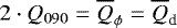$2\cdot Q_{090}={\overline{Q}}_{\varphi }={\overline{Q}}_{\text{d}}$ or all polarized flux of a disk is located only in the left and right quadrants Q₀₉₀ and Q₂₇₀.

Figure 12 includes the relative quadrant parameters measured for HR 4796A from Table 1. This disk has an inclination of about 76° (e.g., Chen et al. 2020; Milli et al. 2019)and the i = 75°-lines match this value well. For Stokes Q_d the front side value $\left|Q_{180}\right|/{\overline{Q}}_{\varphi }$ is very sensitive for the determination of the g-parameter because the corresponding curve in Fig. 12 is steep. This results in a value of g = 0.72 ± 0.03 with a relative uncertainty of only about ±4%, despite the relatively large measuring error of about ±13% for $\left|Q_{180}\right|/{\overline{Q}}_{\varphi }$. The polarization signal is strong near the major axis and the corresponding quadrant values $\left|Q_{090}\right|/{\overline{Q}}_{\varphi }$ and $\left|Q_{270}\right|/{\overline{Q}}_{\varphi }$ can be measured with high precision of roughly ±3%. However, because the $\left|Q_{090}\right|/{\overline{Q}}_{\varphi }$ curve is rather flat in Fig. 12, the resulting uncertainty on the derived g-values is also about ±3%. The obtained g-values for 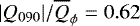$\left|Q_{090}\right|/{\overline{Q}}_{\varphi }=0.62$ and $\left|Q_{270}\right|/{\overline{Q}}_{\varphi }=0.72$ differ significantly because of the described deviation of the HR 4796A disk geometry from axisymmetry.

For the backside quadrant, only an upper limit of about $\left|Q_{000}\right|/{\overline{Q}}_{\varphi }<0.04$ could be measured. This limit is not useful for constraining the g-value because expected values for an inclination of 75° are very low, namely $\left|Q_{000}\right|/{\overline{Q}}_{\varphi }\approx 0.004$ for g = 0.0 and ≈0.001 for g = 0.6, and the corresponding curve is below the plot range covered in Fig. 12.

The relative quadrant values of HR 4796A for Stokes U_d yield low asymmetry parameters g ≈ 0.4 for the back-side quadrants $\left|U_{045}\right|/{\overline{Q}}_{\varphi }$ and $\left|U_{315}\right|/{\overline{Q}}_{\varphi }$, and larger values of g ≈ 0.5 and g ≈ 0.7 for the front side, with again a significant left–right asymmetry.

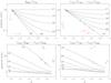Fig. 13 Quadrant polarization ratios for flat disk models for |Q000|∕|Q180|, |U045 |∕|U135|, |Q090 |∕|Q180|, and |Q090|∕|Q135| with measured values from HR 4796A (similar to Fig. 12).

5.2 Quadrant ratios

The scattering asymmetry g can also be derived from quadrant ratios describing the brightness contrast between the front and back sides of the disk as shown in Fig. 13, which includes the measurements from HR 4796A.

High-quality determinations of g are achievedif the front- and the back-side quadrant polarizations can be accurately measured. For low-inclination systems, this should be possible for ratios like |Q₀₀₀|∕|Q₁₈₀| or |U₀₄₅|∕|U₁₃₅| where both the front side and back side are bright. For high-inclination systems, as in HR 4796A, the back side can be faint and the ratios |Q₀₀₀|∕|Q₁₈₀| or |U₀₄₅|∕|U₁₃₅| are small (≲ 0.1) and therefore difficult to measure accurately. As an alternative, one can use ratios based on the bright quadrants like |Q₀₉₀|∕|Q₁₈₀| or |Q₀₉₀|∕|U₁₃₅| or equivalent ratios using the right-side quadrants Q₂₇₀ and U₂₂₅. Many aspects of the diagnostic diagrams plotted in Fig. 13 are similar to the description of the relative quadrant parameters in the previous section.

5.3 Polarized scattering phase function for HR 4796A

5.3.1 Comparison of different g determinations

The measured quadrant polarization parameters for HR 4796A can be used to strongly constrain the asymmetry parameter g of the adopted HG_pol scattering phase function f_ϕ(θ), but only for the θ-range sampled by the used quadrant parameters (see also Hughes et al. 2018). The flux-weighted distribution of scattering angles θ sampled by a quadrant strongly depends on inclination i, but also on g as illustrated in Fig. 14. Indeed, all quadrants of a nearly pole-on disks probe f_ϕ (θ) only near the scattering angle of 90°, while some quadrants probe a large θ-range for strongly inclined disks.

We define the median angle θ_med for the anglethat represents the 50th percentile of a cumulative polarized intensity distribution covered by one quadrant. The back and front quadrants Q₀₀₀ and Q₁₈₀ sample a narrow range, the median angle θ_med is close to the most extreme backward and forward scattering angle θ_med ≈ 90° ± i for a disk with inclination i, and θ_med are essentially identical for different g. The ranges of scattering angles θ covered by the quadrants Q₀₉₀, U₀₄₅, and U₁₃₅ are very broad for larger i and the θ_med depend significantly on g as shown in Fig. 14. For example, θ_med(Q₀₀₀) is 90° for isotropic scattering, and becomes smaller for i → 90° and g → 1 as indicated by the colored θ_med points (diamonds) and the dotted lines.

The quadrants U₀₄₅ and U₁₃₅ sample the back- and front-side parts of the disk and their θ_med-angles lie between those of the Q_d-quadrants. The front-side quadrant also shows a strong tendency towards smaller θ_med(U₁₃₅) values for larger g and i, as in the Q₀₉₀-quadrant, while the g-dependence of θ_med(U₀₄₅) is much smaller.

Figure 15 shows the g-parameters obtained for HR 4796A as a function of the θ-angle probed by the used quadrant parameters. The angle θ corresponds for relative quadrant parameters to θ_med for i = 75° and g = 0.6 as given in Fig. 14 and the horizontal uncertainty bar spans two-thirds of the plotted θ-distribution (from the 16.6 to the 83.3 percentiles). For the quadrant ratios, the adopted θ-values are the mean of the θ_med of the two quadrants and the horizontal bars illustrate their separation. In principle, one should consider for the θ_med-values the systematic trend of g(θ_med) from higher g-values (≈ 0.7) for forward-scattering quadrants to lower values (≈0.4) for the backward scattering quadrants. We neglect this effect which would introduce θ_med shifts of about − 5° for U₁₃₅ and U₂₂₅, shifts of about + 5° for Q₀₉₀ and Q₂₇₀, and smaller shifts for the other quadrants.

Figure 15 shows for HR 4796A a systematic dependence of the derived g-parameters with scattering angle θ. The results from the relative quadrant parameters and the quadrant ratios are roughly consistent. The colors indicate measurements for the left (blue) and right (red) sides of the disk and g-values differ significantly between the two sides for θ_med = 35° and 70° because of the left–right disk brightness asymmetry. On the fainter side, this effect reduces the derived g-value for $U_{225}/{\overline{Q}}_{\varphi }$, while g is enhanced for $Q_{270}/{\overline{Q}}_{\varphi }$ because the intrinsic faintness of Q₂₇₀ mimics a disk with relatively little 90°-scattering because of the normalization with ${\overline{Q}}_{\varphi }$. The intrinsic left–right brightness asymmetry of HR 4796A has less impact on the g determination based on quadrants ratios from the same side. This redundancy helps to disentangle the effects of the scattering asymmetry g from geometric or left–right disk brightness asymmetries.

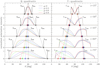Fig. 14 Angular distribution of the polarized intensity in the polarization quadrants for i = 15°, 30°, 45°, 60° and 75° and differentasymmetry parameter g (colors). For quadrants Q000 and Q180 only the caseg = 0 is shown, because differences for other g-parameters are very small. The distributions are normalized for each quadrant individually. For the quadrants Q000, U045, and U135, the median angles θmed (diamonds) for large g-values increase with inclination as illustrated with the dotted lines.

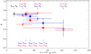Fig. 15 Scattering asymmetry parameters for HR 4796A derived from relative quadrant parameters (open symbols) and quadrant ratios (filled symbols) as a function of the θmed or the mean of θmed, respectively.Colors indicate measurements from the left or SW (blue) and the right or NE (red) disk sides.

Fig. 16 (a) Comparison of the best single parameter HGpol fit model for fixed i = 75° and measured relative quadrant polarization parameters for HR 4796A. (b) Deviations from the best-fitting HGpol (i = 75°, g = 0.65) for the measured values, for the best fits for slightly different disk inclinations HGpol (i = 73°, g = 0.60) and HGpol(i = 77°, g = 0.71) and for the HGpol fit from Milli et al. (2019) (green dashed line). (c) HGpol phase functions and the directly extracted phase function fϕ(θ) (dotted black line) with corresponding uncertainty range (grey shaded area) from Milli et al. (2019). (d) HG intensity phase functions. The measured quadrant values and the different fit curves are identified in panel b.

5.3.2 A “mean” asymmetry parameter g for HR 4796A

The clear trend of the derived g-parameter with scattering angle θ for HR 4796A in Fig. 15 reveals that the used HG_pol-function is an oversimplified description of the polarized scattering phase function for this object. For fainter or less well resolved disks, and for those with low inclination, it may not be possible to recognize such systematic deviations from a HG_pol function, and for all these cases the derived g-value from the HG_pol-function could serve as a good starting point for the analysis of quadrant polarization parameters.

Therefore, for HR 4796A we also derive a “mean” value for the HG asymmetry parameter g despite the discussed trend. To this end, for the seven measured relative quadrant values |U₀₄₅|∕Q_ϕ, |Q₀₉₀|∕Q_ϕ, |U₁₃₅|∕Q_ϕ, |U₁₈₀|∕Q_ϕ, |U₂₂₅|∕Q_ϕ, |U₂₇₀|∕Q_ϕ, and |U₃₁₅|∕Q_ϕ from Table 1, we determine the best-fitting g-asymmetry parameter for the adopted disk inclination i = 75°. This yields HG_pol(i = 75°, g = 0.65) with a weighted sum of squared deviations of χ² = 15.4, and the corresponding calculated and measured values are plotted in Fig. 16a. The differences between the models are more visible in Fig. 16b, where the deviations of data points and calculations from the best-fit model are shown. The large χ² -value indicates that the adopted HG_pol-fit does not describe the data well because of the significant left–right asymmetry between |Q₀₉₀| and |Q₂₇₀|, or |U₁₃₅| and |U₂₂₅| at the level of about 4σ (σ: standard deviations), which cannot be described with an axisymmetric disk model. Additionally, the best fit underestimates the quadrant values at small (θ_med = 16°) and large (124°) scattering angles. Panel b also includes the best-fit results for slightly different disk inclinations HG_pol(i = 73°, g = 0.60) and HG_pol(i = 77°, g = 0.71), which differ very little and produce deviations between fit and data that are similar to the i = 75° solution. The corresponding Henyey-Greenstein scattering phase functions HG_pol (or f_ϕ (θ)) are given in panel c, while panel d shows the HG intensity function (f_I(θ)) for the best quadrant solution for i = 75° and the solution from Milli et al. (2019).

References

- Apai, D., Pascucci, I., Brandner, W., et al. 2004, A&A, 415, 671 [NASA ADS] [CrossRef] [EDP Sciences] [Google Scholar]
- Arriaga, P., Fitzgerald, M. P., Duchêne, G., et al. 2020, AJ, 160, 79 [Google Scholar]
- Artymowicz, P., Burrows, C., & Paresce, F. 1989, ApJ, 337, 494 [NASA ADS] [CrossRef] [Google Scholar]
- Avenhaus, H., Quanz, S. P., Garufi, A., et al. 2018, ApJ, 863, 44 [NASA ADS] [CrossRef] [Google Scholar]
- Bastien, P. 1982, A&AS, 48, 153 [NASA ADS] [Google Scholar]
- Bastien, P., & Menard, F. 1988, ApJ, 326, 334 [NASA ADS] [CrossRef] [Google Scholar]
- Benisty, M., Juhasz, A., Boccaletti, A., et al. 2015, A&A, 578, L6 [NASA ADS] [CrossRef] [EDP Sciences] [Google Scholar]
- Beuzit, J. L., Vigan, A., Mouillet, D., et al. 2019, A&A, 631, A155 [NASA ADS] [CrossRef] [EDP Sciences] [Google Scholar]
- Buenzli, E., & Schmid, H. M. 2009, A&A, 504, 259 [NASA ADS] [CrossRef] [EDP Sciences] [Google Scholar]
- Canovas, H., Ménard, F., de Boer, J., et al. 2015, A&A, 582, L7 [NASA ADS] [CrossRef] [EDP Sciences] [Google Scholar]
- Cantalloube, F., Dohlen, K., Milli, J., Brandner, W., & Vigan, A. 2019, The Messenger, 176, 25 [NASA ADS] [Google Scholar]
- Chen, C., Mazoyer, J., Poteet, C. A., et al. 2020, ApJ, 898, 55 [CrossRef] [Google Scholar]
- Debes, J. H., Weinberger, A. J., & Kuchner, M. J. 2009, ApJ, 702, 318 [NASA ADS] [CrossRef] [Google Scholar]
- de Boer, J., Langlois, M., van Holstein, R. G., et al. 2020, A&A, 633, A63 [NASA ADS] [CrossRef] [EDP Sciences] [Google Scholar]
- Engler, N., Schmid, H. M., Thalmann, C., et al. 2017, A&A, 607, A90 [NASA ADS] [CrossRef] [EDP Sciences] [Google Scholar]
- Esposito, T. M., Kalas, P., Fitzgerald, M. P., et al. 2020, AJ, 160, 24 [Google Scholar]
- Garufi, A., Quanz, S. P., Schmid, H. M., et al. 2016, A&A, 588, A8 [NASA ADS] [CrossRef] [EDP Sciences] [Google Scholar]
- Graham, J. R., Kalas, P. G., & Matthews, B. C. 2007, ApJ, 654, 595 [Google Scholar]
- Hashimoto, J., Tamura, M., Muto, T., et al. 2011, ApJ, 729, L17 [Google Scholar]
- Heikamp, S., & Keller, C. U. 2019, A&A, 627, A156 [NASA ADS] [CrossRef] [EDP Sciences] [Google Scholar]
- Henyey, L. G., & Greenstein, J. L. 1941, ApJ, 93, 70 [Google Scholar]
- Hughes, A. M., Duchêne, G., & Matthews, B. C. 2018, ARA&A, 56, 541 [Google Scholar]
- Hunziker, S., Schmid, H. M., Ma, J., et al. 2021, A&A, 648, A110 [NASA ADS] [CrossRef] [EDP Sciences] [Google Scholar]
- Kalas, P., & Jewitt, D. 1996, AJ, 111, 1347 [NASA ADS] [CrossRef] [Google Scholar]
- Kolokolova, L., & Kimura, H. 2010, A&A, 513, A40 [NASA ADS] [CrossRef] [EDP Sciences] [Google Scholar]
- Macintosh, B., Graham, J. R., Ingraham, P., et al. 2014, Proc. Natl. Acad. Sci., 111, 12661 [NASA ADS] [CrossRef] [Google Scholar]
- Maness, H. L., Kalas, P., Peek, K. M. G., et al. 2009, ApJ, 707, 1098 [NASA ADS] [CrossRef] [Google Scholar]
- Milli, J., Vigan, A., Mouillet, D., et al. 2017, A&A, 599, A108 [NASA ADS] [CrossRef] [EDP Sciences] [Google Scholar]
- Milli, J., Engler, N., Schmid, H. M., et al. 2019, A&A, 626, A54 [NASA ADS] [CrossRef] [EDP Sciences] [Google Scholar]
- Min, M., Rab, C., Woitke, P., Dominik, C., & Ménard, F. 2016, A&A, 585, A13 [NASA ADS] [CrossRef] [EDP Sciences] [Google Scholar]
- Monnier, J. D., Harries, T. J., Bae, J., et al. 2019, ApJ, 872, 122 [Google Scholar]
- Muto, T., Grady, C. A., Hashimoto, J., et al. 2012, ApJ, 748, L22 [Google Scholar]
- Olofsson, J., Milli, J., Bayo, A., Henning, T., & Engler, N. 2020, A&A, 640, A12 [NASA ADS] [CrossRef] [EDP Sciences] [Google Scholar]
- Oppenheimer, B. R., Brenner, D., Hinkley, S., et al. 2008, ApJ, 679, 1574 [NASA ADS] [CrossRef] [Google Scholar]
- Perrin, M. D., Schneider, G., Duchene, G., et al. 2009, ApJ, 707, L132 [Google Scholar]
- Perrin, M. D., Duchene, G., Millar-Blanchaer, M., et al. 2015, ApJ, 799, 182 [Google Scholar]
- Quanz, S. P., Schmid, H. M., Geissler, K., et al. 2011, ApJ, 738, 23 [Google Scholar]
- Schmid, H. M. 2021, IAU Symp., 360, submitted [Google Scholar]
- Schmid, H. M., Joos, F., & Tschan, D. 2006, A&A, 452, 657 [NASA ADS] [CrossRef] [EDP Sciences] [Google Scholar]
- Schmid, H. M., Bazzon, A., Roelfsema, R., et al. 2018, A&A, 619, A9 [NASA ADS] [CrossRef] [EDP Sciences] [Google Scholar]
- Schneider, G., Weinberger, A. J., Becklin, E. E., Debes, J. H., & Smith, B. A. 2009, AJ, 137, 53 [NASA ADS] [CrossRef] [Google Scholar]
- Schneider, G., Debes, J. H., Grady, C. A., et al. 2018, AJ, 155, 77 [Google Scholar]
- Simmons, J. F. L., & Stewart, B. G. 1985, A&A, 142, 100 [NASA ADS] [Google Scholar]
- Tazaki, R., Tanaka, H., Muto, T., Kataoka, A., & Okuzumi, S. 2019, MNRAS, 485, 4951 [NASA ADS] [CrossRef] [Google Scholar]
- Thébault, P. 2009, A&A, 505, 1269 [Google Scholar]
- Tschudi, C., & Schmid, H. M. 2021, A&A, 655, A37 [NASA ADS] [CrossRef] [EDP Sciences] [Google Scholar]
- van Holstein, R. G., Girard, J. H., de Boer, J., et al. 2020, A&A, 633, A64 [NASA ADS] [CrossRef] [EDP Sciences] [Google Scholar]
- Whitney, B. A., & Hartmann, L. 1992, ApJ, 395, 529 [NASA ADS] [CrossRef] [Google Scholar]
- Yudin, R. V., & Evans, A. 1998, A&AS, 131, 401 [NASA ADS] [CrossRef] [EDP Sciences] [Google Scholar]
Defined as in the FORTRAN function atan2(y, x) for Cartesian to polar coordinate conversions.
We distinguish between the polarized flux derived from resolved observations
and unresolved aperture polarimetry
The azimuthal angle φd defined in the disk plane is different from the azimuthal angle ϕxy, which is defined in the sky plane.
Rayleigh scattering produces more forward and backward scattering when compared to isotropic scattering.
All Tables
Measured relative quadrant polarization parameters for HR 4796A, deviations Δ (in %) from left–right symmetry and ratios Λ for back–front flux ratios.
Integration ranges for Stokes Qd and Ud polarization quadrants for on-sky azimuthal angles ϕx,y = atan2(y, x) and disk azimuthal angles φd = atan2(yd, xd).
IDL procedure for the calculation of disk-averaged scattering functions and normalized quadrant polarization parameters.