| Issue |
A&A
Volume 655, November 2021
|
|
|---|---|---|
| Article Number | A82 | |
| Number of page(s) | 10 | |
| Section | Numerical methods and codes | |
| DOI | https://doi.org/10.1051/0004-6361/202039755 | |
| Published online | 23 November 2021 | |
A package for the automated classification of images containing supernova light echoes⋆
1
University of Guelph, Department of Mathematics and Statistics, Guelph, Canada
e-mail: This email address is being protected from spambots. You need JavaScript enabled to view it.
, This email address is being protected from spambots. You need JavaScript enabled to view it.
2
McMaster University, Department of Physics and Astronomy, Hamilton, Canada
e-mail: This email address is being protected from spambots. You need JavaScript enabled to view it.
Received:
24
October
2020
Accepted:
18
October
2021
Abstract
Context. The so-called light echoes of supernovae – the apparent motion of outburst-illuminated interstellar dust – can be detected in astronomical difference images; however, light echoes are extremely rare which makes manual detection an arduous task. Surveys for centuries-old supernova light echoes can involve hundreds of pointings of wide-field imagers wherein the subimages from each CCD amplifier require examination.
Aims. We introduce ALED, a Python package that implements (i) a capsule network trained to automatically identify images with a high probability of containing at least one supernova light echo and (ii) routing path visualization to localize light echoes and/or light echo-like features in the identified images.
Methods. We compared the performance of the capsule network implemented in ALED (ALED-m) to several capsule and convolutional neural networks of different architectures. We also applied ALED to a large catalogue of astronomical difference images and manually inspected candidate light echo images for human verification.
Results. ALED-m was found to achieve 90% classification accuracy on the test set and to precisely localize the identified light echoes via routing path visualization. From a set of 13 000+ astronomical difference images, ALED identified a set of light echoes that had been overlooked in manual classification.
Key words: supernovae: general
ALED is available via github.com/LightEchoDetection/ALED.
© ESO 2021
1. Introduction
Supernovae are extremely luminous but transient events that signal the final stage of a massive star’s evolution or the disruption of a white dwarf in a close binary (Rest et al. 2015). The bright light from the outburst is radiated in all directions and can be scattered by interstellar dust as outburst light encounters such material. The deflection of light off interstellar dust is analogous to the deflection of sound waves off surfaces, hence the term ‘light echo’. Light echoes from a historical supernova can arrive at Earth centuries later than any direct light and consequently they can facilitate the study of historic supernovae in modern times with modern instrumentation. The light echoes of supernovae are present in some astronomical images, but they are almost without exception a small percentage of the surface brightness of the moonless night sky (McDonald 2012).
A difference image is the result of subtracting a pair of images that are taken at the same telescopic pointing, but at different dates. Difference imaging allows for objects that appear to move relative to the background, such as light echoes, to be visually detected more easily (see Fig. 1). However, manual visual image analysis is still demanding due to the large amount of data generated by supernova light echo surveys. For instance, in McDonald (2012), 13 000+ difference images were individually inspected for light echoes over the course of a year.
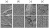 |
Fig. 1. Types of entities present in the CFHT dataset. (a) Images that clearly contain at least one light echo; (b) images that clearly do not contain at least one light echo; (c) images that contain light echoes and artefacts; and (d) images that contain entities with light echo-like characteristics. Illustration and caption credit: Bhullar et al. (2020). |
This paper introduces the Python package ALED (pronounced ‘A-led’) for automated light echo detection in astronomical difference images. This package provides an invaluable resource for astronomers requiring rapid identification of images containing at least one light echo, and where those light echoes are located within the identified images. ALED takes a grey-scale difference image of arbitrary size as input, and outputs a corresponding routing path visualization of the input image (Bhullar et al. 2020). The routing path visualization reveals the regions of the input image that have a high probability of containing a light echo – the brighter the region, the greater the likelihood. Here, we demonstrate and compare the performance of ALED-m, the capsule network model that is available in ALED, to several different artificial neural network classifiers. We also applied ALED to the 13 000+ difference images for which McDonald (2012) did not detect light echoes. ALED was developed specifically for the purpose of light echo detection. Difference imaging also generates artefacts that can, in some instances, mimic the appearance of light echoes, see Fig. 1. Simpler automatic image classification techniques struggle to distinguish light echoes from light-echo-like artefacts (McDonald 2012).
ALED is based on a capsule network (Sabour et al. 2017), which is an extension of a convolutional neural network (CNN). CNNs have achieved state-of-the-art performance on many computer vision problems, and they are currently one of the most popular algorithms for image classification. CNN architectures typically contain millions of weights that are to be learned during training, and as a result, they require a large training set to prevent over-fitting (LeCun et al. 1989). For example, LeNet, a CNN containing 5 978 677 weights, was trained using 60 000 images to classify hand-written digits (LeCun et al. 1998). This particular classification task is considered simpler than light echo detection from difference images because each image is guaranteed to contain a single white digit in the centre of a black background. More complex classification tasks require CNNs with a higher weight count. For example, Wide ResNet-50-2, a CNN containing 68 951 464 weights, was trained using 1.2 million images to classify photographs of 1000 object categories such as boats, horses, etc. (Zagoruyko et al. 2016). This is a more complex classification task because an image can contain one of 1000 coloured objects in an arbitrary orientation on an arbitrary background.
The difficulty of light echo classification falls somewhere in between these two examples. Although there are only two classification categories – a light echo either being present or not – light echoes are not only found in widely different orientations and backgrounds in grey-scale images, but each image may contain several entities, and of those entities, more than one may be a light echo. As such, it is expected that a CNN with millions of weights would be required for adequate light echo detection. In specialized fields, such as observational astronomy, sufficiently large sets of labelled data are often unavailable. This is especially true for automating the classification of images containing supernova light echoes because detectable light echo examples are so few in number (McDonald 2012).
Training a CNN, which contains millions of weights, by using a dataset of a few hundred images is problematic because the model may over-fit to the small dataset in a manner that is not obvious. For example, if the training set represents the validation and test sets well, then the validation and test accuracies will be similar to the training accuracy. However, if the model over-fits to irrelevant characteristics of the dataset, such as camera or pre-processing characteristics or artefacts, then the training, validation, and test accuracies will still be similar even though the model will not perform well on datasets taken by different cameras or pre-processed in a slightly different manner.
Capsule network models require far fewer weights, and thus, are less likely to over-fit to irrelevant characteristics of the dataset. Dropout can be used in CNNs to reduce over-fitting by randomly omitting a certain percentage of neurons every forward propagation step while training. This strategy makes it more difficult for the network to simply memorize the training set or learn unnecessary co-adaptations such as higher-level neurons correcting the mistakes of lower-level neurons (Hinton et al. 2012). For completeness, we include a few CNN architectures to illustrate how many more weights are needed in a CNN compared to a capsule network for light echo detection.
Capsule networks are artificial neural networks that can model hierarchical relationships (Sabour et al. 2017). They typically contain fewer trainable weights than CNNs and, as a result, require a smaller training set to achieve good performance. Capsule networks also facilitate routing path visualization which can be used to interpret the entity that a given capsule detects. Said differently, capsule networks provide a way to see what is being detected. It should be noted that CNNs can also facilitate several gradient-based methods to see what is being detected, such as grad-cam (Selvaraju et al. 2017).
Interpreting how a model functions is important because it will allow for the identification of scenarios that may result in model failure. When the training set is small, as seen in light echo detection, it is expected that the training set will not contain such difficult image classification scenarios even though they are likely to arise in practice. Consequently, constraints can be applied to the network, or improvements can be made to the training set to decrease the probability of failure.
Section 2 describes the Canada-France-Hawaii Telescope (CFHT) difference image data used to train and evaluate ALED. Section 3 briefly reviews capsule networks and describes the network architectures to which ALED was compared and the parameter settings used to classify the 13 000+ CFHT difference images. Section 4 presents the results from the analyses and concluding comments are made in Sect. 5.
2. CFHT dataset
In 2011, CFHT’s wide-field mosaic image, MegaCam, was used to conduct a survey with the primary objective of discovering supernova light echoes in a region where three historical supernovae were known to have occurred. Out of the 13 000+ 2048 × 4612 difference images that were produced from the survey, 22 were found to contain at least one light echo (McDonald 2012). The 22 light echos containing CFHT difference images of size 2048 × 4612 were reduced to 350 difference images of size 200 × 200, among which 175 contained at least a portion of a light echo and the remaining 175 contained other astronomical entities. The dataset was created by manually masking the light echoes present in the 22 images of size 2048 × 4612, which were then cropped to size 200 × 200. If a cropped image contained at least 2500 pixels of mask, then it was classified as containing a light echo.
Among the 4885 200 × 200 cropped images that did not contain a light echo, 175 were selected at random, along with 175 that were classified as containing a light echo to form the final dataset of 350 images. The dataset consists of images and their respective binary labels, where the label indicates whether the image does or does not contain at least one light echo. The dataset was split into a training set of 250 images, and a validation and test set of 50 images each. See Appendix A for a summary of the pre-processing steps required to produce a difference image.
3. Methods
A capsule is a vector whose elements represent the instantiation parameters of an entity in the image, where an entity is defined as an object or object part. The instantiation parameters of an entity are defined as the total information that would be required to render the entity. For example, the instantiation parameters of a circle whose centre is positioned at coordinates (x, y) could be given by (x, y) and the radius of the circle. A capsule network consists of multiple layers of capsules, where a capsule in a given layer detects a particular entity. Capsules in a layer are children to the capsules of its succeeding layer, and a parent to the capsules of its preceding layer. The child-parent coupling of some pairs of capsules is stronger than others, and this is determined by the routing algorithm (Sabour et al. 2017).
Initially, when an image is fed into a capsule network, the image is convolved with a set of filters to produce a feature map, that is to say to produce a tensor representation of the image that is better suited for classification (Goodfellow et al. 2016). The size of the feature map is determined by the length, F, and stride, S, of the filters, and the total number of filters used, N. Higher-level feature maps can be produced from these feature maps, giving rise to M feature maps in total. The Mth feature map is convolved with a set of filters to produce a convolutional capsule (ConvCaps) layer. The ConvCaps layer contains I capsule types each of dimension D, where all capsules of a particular type detect the same entity. The elements of a capsule in the ConvCaps layer are calculated using local regions of the image, so ConvCaps capsules detect simpler entities. Succeeding layer capsules are calculated using preceding layer capsules and transformation weight matrices. Hence, higher-level capsules look at broader regions of the image, and they are expected to detect more complex entities.
Each capsule in the final capsule layer is forced to detect a particular entity, such as a light echo, whilst intermediate layer capsules are not specified to which entities they may detect. The Euclidean length of a capsule will be close to 1 if the entity that the capsule detects is present in the image and close to 0 otherwise. This phenomenon is enforced by minimizing the margin loss while training

where T = 1 if the entity is present in the image and 0 otherwise, m+ = 0.9, ||v|| is the length of the capsule, λ = 0.5, and m− = 0.1 (Sabour et al. 2017). The total margin loss is calculated by summing the margin loss of each capsule in the final capsule layer. If the Euclidean length of the capsule is close to 1, it is said to be ‘active’.
The architecture of ALED-m is shown in Fig. 2. To elaborate, a 200 × 200 image is convolved with a set of 16 filters sized 9 × 9 using a stride of 3 to produce the feature map. The feature map is convolved with a set of 256 filters sized 5 × 5 using a stride of 2 to produce the ConvCaps layer. The subsequent capsule layers contain 24, 8, and 1 capsules of dimensions 12, 16, and 16, respectively. The dimensions of higher-level capsules are larger because more degrees of freedom are required to store the instantiation parameters of more complex entities. The length of the capsule in capsule layer 3 will be close to 1 if a light echo is present in the image, and 0 otherwise. ALED also uses weight sharing in which capsules of the same type within a ConvCaps layer share a set of transformation matrices (Bhullar et al. 2020).
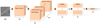 |
Fig. 2. Diagram of the architecture of ALED-m, where ReLU Conv1 is the feature map layer, and Caps1, Caps2, and Caps3 are the capsule layers. |
The entity that a given capsule detects can be localized, if it is present, by routing path visualization (Bhullar et al. 2020). Hence, this technique can be used to interpret the entities detected by intermediate layer capsules. In turn, scenarios can be identified that may result in model failure. For instance, there is one capsule in capsule layer 3, and as a result, the information present in all active capsules in the preceding layer, capsule layer 2, will be strongly routed to that single capsule (Sabour et al. 2017). Consequently, if a capsule(s) in capsule layer 2 is (are) detecting an irrelevant object, such as an artefact, then it (they) may adversely influence predictions made by the light-echo-detecting capsule. Since there is only a single capsule in capsule layer 3, the routing path visualization of that capsule will simply be an addition to the routing path visualizations of the capsules in the preceding layer, capsule layer 2. Changes to the training set or to the model can help ensure that all capsules are detecting sensible objects.
We compared the performance of ALED-m to ten other capsule network architectures (Table 1), and to five CNN models (Table 2) for baseline reference. ALED-m has a similar architecture to model 8, but it contains more filters, capsules, and dimensions per capsule. Models 12 and 13 used the same CNN architecture as model 14, but were trained using augmented training sets of 1000 and 500 images, respectively. The original training set of 250 images was flipped horizontally to create the augmented set of 500 images, and then flipped vertically to create the augmented set of 1000 images in total.
Capsule network architectures trained on the CFHT dataset.
CNN architectures trained on the CFHT dataset.
All models were trained using a single NVIDIA Pascal P100 GPU on TensorFlow (Abadi et al. 2016) with the Adam optimizer (Kingma & Ba 2014). The learning rate was initially set to 0.001 because it was found to be the largest learning rate that caused a steady decline in the total margin loss. If the total margin loss of the validation set had not decreased for ten consecutive iterations, then the learning rate was decreased by a factor of 10. Learning was terminated when the learning rate fell below 10−6. Training was terminated just before the model began over-fitting to the training set. A batch size of 5 was used because it was the largest size that could fit into memory.
An image was classified as containing a light echo if the length of the final capsule was greater than 0.5. The accuracy of the trained model was defined by
and it was found to be 90% on the test set and 88% on the validation set.
4. Results
Using lower weight CNNs (fewer than 5 million weights) was necessary to prevent over-fitting to the small training set (less than 500 images). Regardless, due to the large number of weights in the CNNs relative to the small training set, the two fully connected layers before the output layer required a 95% dropout to combat over-fitting (Table 2). Since dropout is typically set to 50% (Hinton et al. 2012), it may be that too many neurons were initialized in the fully connected layers, thereby resulting in strong over-fitting. Model 15 was trained on the augmented training set of 1000 images to see how a CNN model with less than one million trainable weights, and a more standard percent dropout of 50% would perform.
4.1. Model evaluations
The accuracy and time taken to classify a single image is summarized in Table 3. ALED-m can classify a 200 × 200 difference image in 0.63 seconds, and a corresponding routing path visualization can be produced in approximately 2 seconds. For the capsule network models, it was found that classification accuracy and the time taken to classify an image increased as the number of capsule layers increased. Increasing the number of feature maps, M, and the size of the ConvCaps layer did not noticeably affect the classification accuracy, as demonstrated by models 1, 2, and 3. The total number of trainable weights in a model was mainly influenced by the size of the feature map(s) and ConvCaps layer, and not the number of capsule layers. A notable difference between capsule network and CNN models is that capsule networks can be trained to achieve good classification accuracy using a small non-augmented training set, and an architecture that contains a few thousand trainable weights. For instance, capsule network model 8 and CNN model 12 have a similar accuracy, but model 8 contains 5984 trainable weights whereas model 12 contains 4 551 906.
Prediction accuracy on the validation and test sets is listed for each model.
Figure 3 displays sample routing path visualizations of the capsules in capsule layer 2 for model 8 (Table 1). The brighter the region in a routing path visualization, the more that region of the image is routed to that particular capsule. Capsule 1 seems to be detecting a combination of light echoes and artefacts; capsule 2 seems to be detecting the masked diffraction pattern difference features around bright stars; and capsule 3 seems to be detecting light echoes. Accordingly, the model may fail when given an image of a bright star because capsule 2 will become active, and the irrelevant information contained in capsule 2 will be routed to the light-echo-detecting-capsule. It was found that increasing the number of capsule types, I, and the number of dimensions per capsule, D, resulted in a cleaner routing path visualization. ALED-m and models 6, 8, and 9 had comparable accuracies on both the validation and test sets and performed the best among all capsule network and CNN architectures tested.
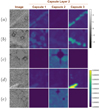 |
Fig. 3. Routing path visualization to interpret the entities that the capsules in capsule layer 2 of model 8 detected. Sample images from test set. Sample test images are of size 200 × 200, and routing path visualizations of capsule layer 2 are of size 29 × 29. Images (a), (b), and (d) contain light echoes; and (c) and (e) contain stars. All images show varying amounts of scattering interstellar dust or artefacts. Illustration and caption credit: Bhullar et al. (2020). |
The absence of artefacts in the routing path visualizations in Fig. 4 in comparison to Fig. 3 reveals that the capsules in capsule layer 2 of ALED-m are not nearly as sensitive to artefacts as model 8. This finding is reasonable because ALED-m is more complex than model 8, and thus, it can learn a more appropriate strategy for classification. All capsules in capsule layer 2 seem to be detecting entities related to light echoes, which makes the model less susceptible to incorrectly classifying a non-light-echo image as a light echo image.
 |
Fig. 4. Routing path visualization to interpret the entities detected by the capsules in capsule layer 2 of ALED-m. Sample images from the test set. On a set of sample test images of size 200 × 200. Routing path visualizations of capsule layer 2 are of size 29 × 29. |
From Fig. 5, it is evident that a routing path visualization of the light-echo-detecting capsule in ALED-m precisely localizes light echoes if they are present in the image. On the contrary, a routing path visualization of the light-echo-detecting capsule in model 8 localizes other entities in addition to light echoes. It seems that a model with more weights can more cleanly localize light echoes in a routing path visualization. In short, model 8 does not always use the correct information in the image to predict the presence of a light echo because irrelevant regions of the image are routed to the light-echo-detecting capsule. Regardless, both model 8 and ALED-m were among the best performing models because of their low misclassification rates (model 8: 5/50, ALED-m: 4/50) and low margin loss (model 8: 0.037, ALED-m: 0.039). These models could better distinguish light echoes from artefacts compared to most other models. See Table B.1 for classification details for select models.
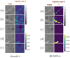 |
Fig. 5. Routing path visualization to localize light echoes detected by the light-echo-detecting capsule. Sample images from the test set. Sample test images are of size 200 × 200, and routing path visualizations of capsule layer 3 are of size 29 × 29. |
4.2. ALED classification results
ALED-m was found to have fewer false positives if the classification was based on the routing path visualization pixel value, rather than on the length of the light-echo-detecting capsule. As such, if a routing path visualization contains at least one pixel with a value greater than 0.00042, then ALED classifies the corresponding difference image as a light echo candidate. However, this threshold can be changed to increase or decrease the pool of light echo candidates. ROC and precision-recall curves were generated by varying the classification threshold from 0 to 0.00070 (Fig. B.1), and then applying ALED-m to the entire set of 350 cropped CFHT images of size 200 × 200. The confusion matrix corresponding to a threshold of 0.00042 shows that there are no false positives, so ALED-m is able to identify light echos with a specificity of 1 (Table 4 and Figs. 6c–e). It was found that very faint and narrow light echoes may get falsely classified as non-light-echoes (Figs. 6a and b).
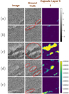 |
Fig. 6. Sample of routing path visualizations of five light echos. (a)–(b) Classified as ‘no light echo’; and (c)–(e) classified as ‘light echo’. Red ellipses localize light echoes. |
Number of true positive (TP), true negative (TN), false positive (FP), and false negative (FN) classifications based on ALED-m.
All 13 000+ 2048 × 4612 difference images produced in 2011 by CFHT’s MegaCam, including the 22 images that were used to train ALED-m, were also classified by ALED. When input images are larger than 200 × 200, ALED pads the input image so that it is completely divisible into 200 × 200 sub-images. Each sub-image is passed through ALED-m, and a corresponding routing path visualization is produced. The routing path visualizations are stitched together into a final routing path visualization.
From the 13 000+ difference images, 1646 images were classified to be light echo candidates. The 1646 difference images were then manually inspected for validation, which was a two-hour process, and one difference image was found to contain bona fide Cas A light echoes not noted by McDonald (2012), see Fig. 7e. The significance of this finding is that the ALED algorithm was able to identify a group of light echoes that were not in the training set.
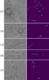 |
Fig. 7. Difference images and their corresponding routing path visualizations. (a)–(d) Sample artefacts that ALED classified as light echo candidates; and (e) Cas A light echoes that ALED correctly classified. |
About 40% of the light echo candidates from the classification of all available difference images were due to bright stars, see Fig. 7a. There are always small pointing differences between the two images used to create a difference image. The diffraction patterns around bright stars are then slightly displaced and when differenced, show radially displaced patterns that can be mistaken for very sharp, low apparent motion, light echo features. This misclassification is reasonable because bright star artefacts are large, usually spanning a 1000 × 1000 pixel region of an image, and ALED only looks at local 200 × 200 regions of an image at a time. Fortunately, since the positions and apparent brightness of such stars are known, bright stars can be algorithmically filtered from the pool of light echo candidates. Figures 7b–d show the routing path visualizations of rejected light echo candidates, all of which exhibit light echo-like features. Apparently, several such features were contained in the training set, but ALED correctly assessed them as unlikely light echo candidates.
5. Summary
We have presented ALED, a novel tool for the automated classification of light echoes from differenced astronomical images. ALED uses capsule networks for classification and routing path visualization to localize regions of the image contributing to the classification. The performance of ALED is competitive with CNNs, but it requires far fewer training weights or training samples, and it does not rely on either drop out or augmenting the training set with training image transpositions. For practitioners, the routing path visualizations facilitate the quick identification of class entities within an image.
Model ALED-m was implemented in the Python package ALED and was trained on the CFHT data to predict the presence of light echoes in astronomical images. ALED-m uses the correct regions of an image when predicting the presence of light echo and can precisely localize light echoes when they are present in an image. The arduous task of classifying 13 000+ images by manual inspection was drastically reduced by applying ALED-m to identify light echo candidates and then using manual inspection for confirmation only on the set of light echo candidates. Further, one novel light echo image was detected by ALED-m that had been missed by manual classification.
Although ALED uses a capsule network to improve its generalizability, future work involves testing ALED on astronomical images not taken from the CFHT MegaCam. The Python package ALED is publicly available1, though corresponding package documentation is also provided in Appendix C. To the authors’ knowledge, this is the first automation of the laborious task of light echo detection.
Acknowledgments
We are grateful to Dr. Armin Rest (STScI) for the preparation of the difference images from the CFHT MegaCam survey. This research was enabled in part by support provided by Compute Ontario (www.computeontario.ca) and Compute Canada (www.computecanada.ca). The images analysed were based on observations obtained with MegaPrime/MegaCam, a joint project of CFHT and CEA/DAPNIA, at the Canada-France-Hawaii Telescope (CFHT) which is operated by the National Research Council (NRC) of Canada, the Institut National des Sciences de l’Univers of the Centre National de la Recherche Scientifique of France, and the University of Hawaii. This research was supported by the National Science and Engineering Research Council of Canada.
References
- Abadi, M., Agarwal, A., Barham, P., et al. 2016, ArXiv e-prints [arXiv:1603.04467] [Google Scholar]
- Bhullar, A., Ali, R. A., & Welch, D. L. 2020, Interpreting capsule networks for image classification by routing path visualization (University of Guelph) [Google Scholar]
- Goodfellow, I., Bengio, Y., & Courville, A. 2016, Deep Learning, 1 (MIT press Cambridge) [Google Scholar]
- Hinton, G. E., Srivastava, N., Krizhevsky, A., Sutskever, I., & Salakhutdinov, R. R. 2012, ArXiv e-prints [arXiv:1207.0580] [Google Scholar]
- Kingma, D. P., & Ba, J. 2014, ArXiv e-prints [arXiv:1412.6980] [Google Scholar]
- LeCun, Y., Boser, B., Denker, J. S., et al. 1989, Neural Comput., 1, 541 [NASA ADS] [CrossRef] [Google Scholar]
- LeCun, Y., Bottou, L., Bengio, Y., & Haffner, P. 1998, Proc. IEEE, 86, 2278 [Google Scholar]
- McDonald, B. J. 2012, The search for supernova light echoes from the core-collapse supernovae of AD 1054 (crab) and AD 1181 (master’s thesis), (McMaster University) [Google Scholar]
- Rest, A., Stubbs, C., Becker, A. C., et al. 2005, ApJ, 634, 1103 [NASA ADS] [CrossRef] [Google Scholar]
- Rest, A., Sinnott, B., Welch, D. L., et al. 2015, in Fifty Years of Wide Field Studies in the Southern Hemisphere: Resolved Stellar Populations of the Galactic Bulge and Magellanic Clouds, eds. S. Points, A. Kunder, et al., ASP Conf. Ser., 491, 247 [NASA ADS] [Google Scholar]
- Sabour, S., Frosst, N., & Hinton, G. E. 2017, Advances in Neural Information Processing Systems, 3856 [Google Scholar]
- Schechter, P. L., Mateo, M., & Saha, A. 1993, PASP, 105, 1342 [Google Scholar]
- Selvaraju, R. R., Cogswell, M., Das, A., et al. 2017, in Proceedings of the IEEE international conference on computer vision, 618 [Google Scholar]
- Shang, Z., Hu, K., Hu, Y., et al. 2012, in Observatory Operations: Strategies, Processes, and Systems IV, International Society for Optics and Photonics, 8448, 844826 [NASA ADS] [CrossRef] [Google Scholar]
- Zagoruyko, S., & Komodakis, N. 2016, in Proceedings of the British Machine Vision Conference (BMVC), eds. E. R. H. Richard, C. Wilson, & W. A. P. Smith (BMVA Press), 87.1 [Google Scholar]
Appendix A: Reduction and difference-imaging technique (McDonald 2012)
This appendix summarizes the pre-processing of astronomical photos to produce the differenced images on which ALED was trained. Difference-imaging involves the digital image subtraction of two or more epochs of the same field or viewpoint. McDonald (2012) developed an image pipeline that used reduced CFHT images and adapted a technique by Rest et al. (2005) to perform the differencing. A brief description of the difference-imaging steps implemented by the image pipeline on the reduced images are described below:
-
Deprojection - Each image was re-sampled to the same geometry as the template image (earlier epoch image) so that images were photometrically aligned to facilitate subtraction per the SWarp software package (Shang et al. 2012).
-
Aperture photometry - The reduced and re-sampled images were photometrically calibrated using the DoPHOT photometry package to identify and measure sources (Schechter et al. 1993), and identify a photometric zero point for the image.
-
Pixel masking - Saturated pixels were masked out since their true brightness values are unknown (i.e. for saturated stars, both the star and its spikes were masked).
-
Image subtraction - Clean difference images were produced by point-spread-function (PSF) matching and then subtracting pixel values, using the Higher Order Transform of PSF and Template Subtraction (HOTPANTS) package.
The photometric alignment and PSF matching are the most difficult steps of this process. Indeed, the images to be subtracted are often taken under different conditions, including atmospheric transparency, atmospheric seeing, or exposure times, with each image consequently having a different PSF. A convolution kernel that matches the PSFs of two astronomical images is found such that the output pixel is a weighted sum of the input pixels within a kernel of a certain size. Further, since the PSF of astronomical images are spatially varied, the kernel must be modelled as a spatially varying function (McDonald 2012).
Appendix B: Extended model evaluation
Here we present further classification results. Table B.1 compares classification using different capsule and CNN architectures for the classification threshold based on the length of light-echo-detecting capsule. Lower model loss was typically associated with a better ability to distinguish light echoes from light-echo-like artefacts. Figure B.1 plots performance curves for model ALED-m, using the classification threshold based on the routing path visualization pixel value.
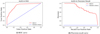 |
Fig. B.1. ROC and precision-recall curve of ALED-m as calculated by varying the threshold of 0.00042 from 0 to 0.00070. |
Classification (TP: true positive, TN: true negative, FP: false positive, FN: false negative) of the test set of 50 images for several models.
Appendix C: Package documentation - github.com/LightEchoDetection/ALED
This appendix provides details on how to use the ALED package and perform routing path visualization in Python. The function classify_fits() takes as input the path of a directory containing difference images, of any size, to be classified. Each difference image is cropped to many images of size 200 × 200, which are then classified and a corresponding routing path visualization is produced. The routing path visualizations are stitched together to form a final output routing path visualization that corresponds to the input image. The routing path visualization localizes the light echoes for the user. The output also includes a text file listing images that are good candidates for containing a light echo.
C.1. Installation
-
Install Python 3.7.
-
(Optional) create a virtual environment, virtualenv aledpy, and an activate virtual environment, source aledpy/bin/activate.
-
Install the jupyter notebook, pip install jupyterlab.
-
Install dependencies via pip install ...
Dependencies: astropy==3.0.5
matplotlib==3.0.2
numpy==1.16.3
opencv-python==3.4.4.19
pandas==0.24.1
scikit-image==0.14.2
scikit-learn==0.20.2
scipy==1.2.1
tensorflow-gpu==1.11.0 or tensorflow==1.11.0
Installing tensorflow-gpu==1.11.0 is not a straight forward pip install tensorflow-gpu==1.11.0, instead follow this tutorial https://www.tensorflow.org/install/gpu. tensorflow==1.11.0 can be installed easily using pip, however, it is typically much slower than tensorflow-gpu because it only uses the cpu.
-
Run the jupyter notebook, jupyter notebook. If you are remotely connected to the computer, then port forward jupyter notebook onto your local computer via local_user@local_host$ ssh -N -f -L localhost:8888:localhost:8889 remote_user@remote_host. 6. To make sure everything is installed correctly, run test.ipynb.
C.2. Description
The test.ipynb file contains sample code to get you started. Call function classify_fits(snle_image_paths, snle_names, start) from file model_functions.py to start the classification process. snle_image_paths is a Python list of the file paths of each differenced image to be classified (each image in .fits format). snle_names is a Python list of the names of the images corresponding to the file paths (names can be arbitrary strings). start is an int that allows you to start the classification process where you left off in case the process has to be terminated.
The input image is cropped to multiple 200x200 sub-images (we note that padding is added to the input image so that it is completely divisible by 200x200). Each sub-image is passed through the network for classification, and a corresponding routing path visualization image is produced. The routing path visualization images are stitched together and saved as a .png in directory astro_package_pics/, along with the input image.
For each .fits image, a corresponding routing path visualization image is saved to astro_package_pics/. In addition, a text file titled snle_candidates.txt is created. The text file contains the name of each .fits file, and five values called Count1, Count2, Count3, Avg1, and Avg2, representing the likelihood of the image containing a light echo. From experience, if Count1 is non-zero, then the image should be considered a light echo candidate.
-
Count1: A count of the number of pixels in the routing path visualization image that have a value greater than 0.00042.
-
Count2: A count of the number of pixels in the routing path visualization image that have a value greater than 0.00037.
-
Count3: A count of the number of pixels in the routing path visualization image that have a value greater than 0.00030.
-
Avg1 is the average length of the light-echo-detecting capsule for the top_n sub-images with the largest length for the light-echo-detecting capsule.
-
Avg2 is the average length of the light-echo-detecting capsule for the small_n sub-images with the largest length for the light-echo-detecting capsule.
As default, top_n=45 and small_n=10. top_n and small_n are arguments for classify_fits() and can be changed via classify_fits(..., top_n=45, small_n=10).
C.3. Test package
To check if the dependencies have been installed correctly, open test.ipynb and run all cells. If successful, the following three files should be produced:
-
snle_candidates.txt: It contains the following line test.fits 375.000000 440.000000 562.000000 0.731215 0.880019.
-
astro_package_pics/rpv_test.fits.png: The routing path visualization image of test.fits
-
astro_package_pics/snle_test.fits.png: test.fits in .png format
C.4. Re-train model
The user must have a dataset in order to re-train the model as one is not provided. The re-training script is entitled retrain_script.ipynb in this repository. We recommend that the dataset contain an equal number of light echo and non-light-echo images to prevent any class imbalance issues that may arise. The script demonstrates how to train a new model with the same architecture as ALED-m, and starting from the weights learned by ALED-m.
All Tables
Number of true positive (TP), true negative (TN), false positive (FP), and false negative (FN) classifications based on ALED-m.
Classification (TP: true positive, TN: true negative, FP: false positive, FN: false negative) of the test set of 50 images for several models.
All Figures
|
Fig. 1. Types of entities present in the CFHT dataset. (a) Images that clearly contain at least one light echo; (b) images that clearly do not contain at least one light echo; (c) images that contain light echoes and artefacts; and (d) images that contain entities with light echo-like characteristics. Illustration and caption credit: Bhullar et al. (2020). |
| In the text | |
|
Fig. 2. Diagram of the architecture of ALED-m, where ReLU Conv1 is the feature map layer, and Caps1, Caps2, and Caps3 are the capsule layers. |
| In the text | |
|
Fig. 3. Routing path visualization to interpret the entities that the capsules in capsule layer 2 of model 8 detected. Sample images from test set. Sample test images are of size 200 × 200, and routing path visualizations of capsule layer 2 are of size 29 × 29. Images (a), (b), and (d) contain light echoes; and (c) and (e) contain stars. All images show varying amounts of scattering interstellar dust or artefacts. Illustration and caption credit: Bhullar et al. (2020). |
| In the text | |
|
Fig. 4. Routing path visualization to interpret the entities detected by the capsules in capsule layer 2 of ALED-m. Sample images from the test set. On a set of sample test images of size 200 × 200. Routing path visualizations of capsule layer 2 are of size 29 × 29. |
| In the text | |
|
Fig. 5. Routing path visualization to localize light echoes detected by the light-echo-detecting capsule. Sample images from the test set. Sample test images are of size 200 × 200, and routing path visualizations of capsule layer 3 are of size 29 × 29. |
| In the text | |
|
Fig. 6. Sample of routing path visualizations of five light echos. (a)–(b) Classified as ‘no light echo’; and (c)–(e) classified as ‘light echo’. Red ellipses localize light echoes. |
| In the text | |
|
Fig. 7. Difference images and their corresponding routing path visualizations. (a)–(d) Sample artefacts that ALED classified as light echo candidates; and (e) Cas A light echoes that ALED correctly classified. |
| In the text | |
|
Fig. B.1. ROC and precision-recall curve of ALED-m as calculated by varying the threshold of 0.00042 from 0 to 0.00070. |
| In the text | |
Current usage metrics show cumulative count of Article Views (full-text article views including HTML views, PDF and ePub downloads, according to the available data) and Abstracts Views on Vision4Press platform.
Data correspond to usage on the plateform after 2015. The current usage metrics is available 48-96 hours after online publication and is updated daily on week days.
Initial download of the metrics may take a while.