| Issue |
A&A
Volume 655, November 2021
|
|
|---|---|---|
| Article Number | A38 | |
| Number of page(s) | 12 | |
| Section | Astrophysical processes | |
| DOI | https://doi.org/10.1051/0004-6361/202039268 | |
| Published online | 09 November 2021 | |
Cross-sections of relativistic quantum-mechanical versus those of classical magnetic resonant scattering
1
University of Crete, Department of Physics & Institute of Theoretical & Computational Physics, 70013 Heraklion, Greece
e-mail: kylafis@physics.uoc.gr
2
Institute of Astrophysics, Foundation for Research and Technology-Hellas, 71110 Heraklion, Crete, Greece
3
Max-Planck-Institut für extraterrestrische Physik, Postfach 1312, 85741 Garching, Germany
Received:
26
August
2020
Accepted:
27
July
2021
Context. Radiative transfer calculations in strong (few ×1012 G) magnetic fields, which are observed in X-ray pulsars, require accurate differential cross-sections of resonant scattering. While such cross-sections exist, their application is cumbersome.
Aims. Here, we compare the classical (non-relativistic) with the quantum-mechanical (relativistic) resonant differential scattering cross-sections and offer a prescription for the use of the much simpler classical expressions with impressively accurate results.
Methods. We expanded the quantum-mechanical differential cross-sections and kept the terms up to the first order in ϵ ≡ E/mec2 and B ≡ ℬ/ℬcr, where E is the photon energy and ℬcr is the critical magnetic field. We recovered the classical differential cross-sections along with the terms that are due to spin flip, which is a pure quantum-mechanical phenomenon.
Results. When adding the spin-flip terms to the polarization-dependent classical differential cross-sections by hand, we find that they are in excellent agreement with the quantum mechanical ones for all energies near resonance and all angles. We plotted both of them and the agreement is impressive.
Conclusions. We give a prescription for the use of the classical differential cross-sections for radiative transfer calculations that guarantees accurate results.
Key words: accretion / accretion disks / scattering / stars: magnetic field / pulsars: general / X-rays: stars
© ESO 2021
1. Introduction
Cyclotron lines are prominent features in the spectra of X-ray pulsars. The first cyclotron line was discovered in Hercules X-1 (Trümper et al. 1977, 1978) and since then, over 35 accreting magnetic neutron stars exhibit electron cyclotron lines have been found, sometimes with their harmonics (Staubert et al. 2019). They are also called cyclotron resonance scattering features (CRSFs).
Despite the many years that have passed since the first observation of a CRSF, it is still unclear where these features form and what type of mechanism produces them. Early on, it was suggested (Basko & Sunyaev 1976) that the CRSFs are produced in the radiative shock in the accretion column. However, no calculation has been done so far for the simultaneous production of the power-law spectrum and the cyclotron line in a radiative shock. Instead, several calculations have been performed using a slab that is illuminated from one side (Ventura 1979; Nagel 1981; Nishimura 2008; Araya & Harding 1999; Araya-Góchez & Harding 2000; Schönherr et al. 2007).
Another interesting idea was given by Poutanen et al. (2013), who proposed that the CRSF is produced as a result of the reflection of the continuum emitted at the radiative shock on the surface of the neutron star. Again, no radiative transfer calculation has been reported on this mechanism thus far.
A possible reason for the limited detailed calculations is the resonant differential cross-sections. It is not a question of their unavailability, but of their complexity. The expressions derived by Herold (1979), Daugherty & Harding (1986), Bussard et al. (1986), Harding & Daugherty (1991), Sina (1996), Gonthier et al. (2014), Mushtukov et al. (2016), Schwarm (2017) for the complete, quantum electrodynamic, differential Compton resonant cross-sections are quite general and because of this, they can prove cumbersome and rather impractical. However, this generality is not needed in most cases.
Most of the cyclotron lines that have been observed thus far (for a review see Staubert et al. 2019) are at cyclotron energies Ec ≪ mec2, implying magnetic fields of ℬ ≪ ℬcr, where  is the critical magnetic field. For such cases, an expansion of the full quantum mechanical cross-sections up to first order in ϵ ≡ E/mec2 and B ≡ ℬ/ℬcr gives simpler, but nevertheless accurate, expressions for the necessary calculations.
In the literature, we can find the much simpler classical (Thomson) cross-sections (Canuto et al. 1971; Blandford & Scharleman 1976; Nobili et al. 2008a). The question then arises regarding whether a prescription can be found making use of the simple classical cross-sections in radiative transfer calculations to give highly accurate results. The present work answers this question with a positive assessment of this possibility.
In Sect. 2, we discuss the polarization-dependent cross-sections. First, we give the classical ones. Then, we discuss the quantum-mechanical cross-sections that have been derived either with the Johnson & Lippmann (1949) wave functions or with the physically more meaningful Sokolov & Ternov (1968) formalism, and we compare them numerically for E ≪ mec2 and ℬ ≪ ℬcr. We expand, to first order with regard to the small parameters, ϵ and B, the cross-sections given by Harding & Daugherty (1991) and Sina (1996). Finally, we offer a prescription that allows for the classical cross-sections to be used to obtain highly accurate results. In Sect. 3, we summarize our findings of our work.
2. Cross-sections
2.1. Classical
The classical (Thomson) differential cross-sections for polarized resonant scattering are given by Nobili et al. (2008a; see also Canuto et al. 1971; Blandford & Scharleman 1976). After integrating over the azimuthal angle ϕ, we have:
where the index 1 (2) stands for the ordinary (extraordinary) mode, r0 is the classical electron radius, and
is the normalized Lorentz profile, with ω = E/ℏ as the photon frequency and ωr = Er/ℏ the resonant frequency, which in the non-relativistic regime, is the cyclotron frequency ωc = eℬ/mec,  , accounting for the finite transition life-time of the excited state (e.g. Daugherty & Ventura 1978; Ventura 1979). Finally, θ and θ′ are the incident and scattered angles, respectively, with respect to the direction of the magnetic field ℬ.
The polarization averaged differential cross-section is given by

2.2. Relativistic quantum mechanical
Expressions for the differential Compton scattering cross-sections as functions of polarization, energy, E, and magnetic field, ℬ, have been derived by Harding & Daugherty (1991), using the Johnson & Lippmann (1949) wave functions. Similar, albeit more accurate, expressions have been derived by Sina (1996) using the Sokolov & Ternov formalism (for a detailed discussion see Gonthier et al. 2014). At large values of ℬ, there are differences between the two (Schwarm 2017).
Since we are interested at non-relativistic energies and sub-critical magnetic fields, we carry out a numerical comparison of the expressions of Harding & Daugherty (1991) with those of Sina (1996) for B = 0.03. In Fig. 1, we compare dσ11/d cos θ′ near-resonance for four values of the incident angle θ, with respect to the magnetic field, and four values of the scattered angle θ′. The black lines correspond to Harding & Daugherty (1991), while the red ones to Sina (1996). The curves essentially overlap, but for a detailed comparison “at resonance,” we show in Fig. 2 the ratio of the two curves for the cases displayed in Fig. 1. The differences at resonance are less than 3%. We remark that a similar agreement exists for the other three differential cross-sections.
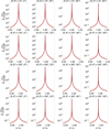 |
Fig. 1. Polarization-dependent differential cross-section (1/σT) dσ11/d cos θ′ as a function of photon energy E = ℏω for a set of incident angles θ and scattered angles θ′. The set of angles is 0, 30, 60, and 90 degrees, with θ changing vertically and θ′ horizontally. The red solid lines are produced from the expression of Sina (1996), while the black dashed ones are produced from the expression of Harding & Daugherty (1991). In all cases, the resonant frequency is given by expression (7). The vertical line indicates the resonant frequency ωr, which for θ ≠ 0 is smaller than ωc. Here, Ec = ℏωc = 15.33 keV. |
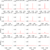 |
Fig. 2. Ratio of the Harding & Daugherty (1991) polarization-dependent differential cross-section (1/σT) dσ11/d cos θ′ to that of Sina (1996) for the cases shown in Fig. 1. |
In Fig. 3, we show in the form of heat maps the ratios “at resonance” of the differential cross-sections calculated from the expressions of Harding & Daugherty (1991) to those of Sina (1996) for B = 0.03. It is evident that, for all incident angles θ and all scattered angles θ′, the ratio is between 1.000 and 1.027. Thus, for B ≪ 1, it is irrelevant which of the two formalisms is used.
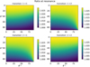 |
Fig. 3. Ratio of the Harding & Daugherty (1991) polarization-dependent differential cross-sections at resonance to those of Sina (1996) for different incident and scattered angles θ and θ′, respectively. In all cases, the resonant frequency is given by Eq. (7) and B = 0.03. |
In order to find simpler expressions, that are nevertheless accurate for E ≪ mec2 and ℬ ≪ ℬcr, we expanded the expressions of Harding & Daugherty (1991) to first order in the small parameters, ϵ = E/mec2 and B = ℬ/ℬcr. This is shown in Appendix A. Here, we give the results:
![$$ \begin{aligned} { {\mathrm{d} \sigma _{11}} \over {\mathrm{d}\cos \theta ^\prime } }&= 2\pi { {3\pi r_o c} \over {8} }\Bigg [ g^{1 \rightarrow 1} \cdot L_{-} + h^{1 \rightarrow 1} \cdot L_{+}\nonumber \\&\quad + \sqrt{2 B} \cos \theta \cos \theta ^\prime \dfrac{L_{-} \cdot L_{+}}{L_{\rm mix}} \Bigg ],\end{aligned} $$](/articles/aa/full_html/2021/11/aa39268-20/aa39268-20-eq9.gif)
![$$ \begin{aligned} { {\mathrm{d} \sigma _{12}} \over {\mathrm{d}\cos \theta ^\prime } }&= 2\pi { {3\pi r_o c} \over {8} }\Bigg [g^{1 \rightarrow 2} \cdot L_{-} + h^{1 \rightarrow 2} \cdot L_{+} \nonumber \\&\quad + \sqrt{2 B} \cos \theta \cos \theta ^\prime \dfrac{L_{-} \cdot L_{+}}{L_{\rm mix}} \Bigg ],\end{aligned} $$](/articles/aa/full_html/2021/11/aa39268-20/aa39268-20-eq10.gif)
![$$ \begin{aligned} { {\mathrm{d} \sigma _{21}} \over {\mathrm{d}\cos \theta ^\prime } }&= 2\pi { {3\pi r_o c} \over {8} }\Bigg [g^{2 \rightarrow 1} \cdot L_{-} + h^{2 \rightarrow 1} \cdot L_{+} \nonumber \\&\quad + \sqrt{2 B} \cos \theta \cos \theta ^\prime \dfrac{L_{-} \cdot L_{+}}{L_{\rm mix}} \Bigg ],\end{aligned} $$](/articles/aa/full_html/2021/11/aa39268-20/aa39268-20-eq11.gif)
![$$ \begin{aligned} { {\mathrm{d} \sigma _{22}} \over {\mathrm{d}\cos \theta ^\prime } }&= 2\pi { {3\pi r_o c} \over {8} }\Bigg [ g^{2 \rightarrow 2} \cdot L_{-} + h^{2 \rightarrow 2} \cdot L_{+} \nonumber \\&\quad + \sqrt{2 B} \cos \theta \cos \theta ^\prime \dfrac{L_{-} \cdot L_{+}}{L_{\rm mix}} \Bigg ], \end{aligned} $$](/articles/aa/full_html/2021/11/aa39268-20/aa39268-20-eq12.gif)
where L−(ω, ωr), L+(ω, ωr) and Lmix(ω, ωr) are the normalized Lorentz profiles, which are characterized by the decay widths  , and
, and  , respectively, and are given in Appendix A. The resonant frequency ωr is given in Eq. (7) below. In addition,
  and
and  are first-degree polynomials in B, and are given in Appendix A. We note that s represents the polarization mode of the incident photon, whereas s′ represents that of the scattered photon.
In Appendix B, we expanded the expressions of Sina (1996) to first order in ω = E/(ℏmec2) and B = ℬ/ℬcr. The results are as follows:
![$$ \begin{aligned} { {\mathrm{d} \sigma _{11}} \over {\mathrm{d}\cos \theta ^\prime } }&= 2\pi { {3\pi r_o c} \over {8} }\Bigg [ \mathcal{{G}}^{1 \rightarrow 1} \cdot L_{-} + h^{1 \rightarrow 1} \cdot L_{+} \nonumber \\&\quad + \sqrt{2 B} \cos \theta \cos \theta ^\prime \dfrac{L_{-} \cdot L_{+}}{L_{\rm mix}} \Bigg ],\end{aligned} $$](/articles/aa/full_html/2021/11/aa39268-20/aa39268-20-eq17.gif)
![$$ \begin{aligned} { {\mathrm{d} \sigma _{12}} \over {\mathrm{d}\cos \theta ^\prime } }&= 2\pi { {3\pi r_o c} \over {8} }\Bigg [\mathcal{{G}}^{1 \rightarrow 2} \cdot L_{-} + h^{1 \rightarrow 2} \cdot L_{+}\nonumber \\&\quad + \sqrt{2 B} \cos \theta \cos \theta ^\prime \dfrac{L_{-} \cdot L_{+}}{L_{\rm mix}} \Bigg ],\end{aligned} $$](/articles/aa/full_html/2021/11/aa39268-20/aa39268-20-eq18.gif)
![$$ \begin{aligned} { {\mathrm{d} \sigma _{21}} \over {\mathrm{d}\cos \theta ^\prime } }&= 2\pi { {3\pi r_o c} \over {8} }\Bigg [ \mathcal{{G}}^{2 \rightarrow 1} \cdot L_{-} + h^{2 \rightarrow 1} \cdot L_{+} \nonumber \\&+ \sqrt{2 B} \cos \theta \cos \theta ^\prime \dfrac{L_{-} \cdot L_{+}}{L_{\rm mix}} \Bigg ],\end{aligned} $$](/articles/aa/full_html/2021/11/aa39268-20/aa39268-20-eq19.gif)
![$$ \begin{aligned} { {\mathrm{d} \sigma _{22}} \over {\mathrm{d}\cos \theta ^\prime } }&= 2\pi { {3\pi r_o c} \over {8} }\Bigg [ \mathcal{{G}}^{2 \rightarrow 2} \cdot L_{-} + h^{2 \rightarrow 2} \cdot L_{+}\nonumber \\&\quad + \sqrt{2 B} \cos \theta \cos \theta ^\prime \dfrac{L_{-} \cdot L_{+}}{L_{\rm mix}} \Bigg ], \end{aligned} $$](/articles/aa/full_html/2021/11/aa39268-20/aa39268-20-eq20.gif)
where L−(ω, ωr), L+(ω, ωr), Lmix(ω, ωr), and  are the same as in Eqs. (4a)–(4d), while the correction functions
  are slightly different from the
  ones and are given in Appendix B. We note that in order to avoid confusion between the different notations, we employed the notation of Harding & Daugherty (1991) in Eqs. (5a)–(5d) instead of the notation of Sina (1996), which we systematically use in Appendix B.
It is important to notice two things: (a) the similarity of the expressions in Eqs. (5a)–(5d) with those of Eqs. (4a)–(4d); they are identical, except for the small differences between g and 𝒢. This, of course, is not surprising given the ratio plots in Fig. 2 and the heat plots in Fig. 3. (b) The expressions in Eqs. (4a)–(4d) and (5a)–(5d) are much simpler than the full expressions given by Harding & Daugherty (1991) and Sina (1996), respectively.
2.3. Even simpler expressions
Looking at the expressions in Eqs. (4a)–(4d) and (5a)–(5d), we considered whether all the terms in them are crucial. Thus, we wrote down the extremely simple expressions, as follows:

The terms proportional to L− are identical to the classical cross-sections Eqs. (1a)–(1d), because L− is equal to L given by Eq. (2). The terms proportional to L+ are non-classical because they contain the decay width Γ+, which is associated with the spin flip.
In Fig. 4, we compare expression (6b) with expression (5b) for B = 0.03 and in Fig. 5, we present the ratio of these two formulae. The differences are impressively negligible. The same is true for the heat maps “at resonance” (Fig. 6).
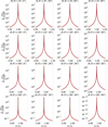 |
Fig. 4. Polarization-dependent resonant differential cross-section (1/σT) dσ12/d cos θ′ as a function of photon energy E = ℏω for a set of incident angles θ and scattered angles θ′. The set of angles is 0, 30, 60, and 90 degrees, with θ changing vertically and θ′ horizontally. The red solid lines are produced from the first order expansion (5b) of Sina (1996), while the black dashed ones are produced from the simplified expression (6b). In all cases, the resonant frequency is given by Eq. (7). The vertical line indicates the resonant frequency ωr, which for θ ≠ 0 is smaller than ωc. Here, Ec = ℏωc = 15.33 keV. |
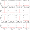 |
Fig. 5. Ratio of the polarization-dependent differential cross-sections dσ12/d cos θ′ given by (5b) to the simplified expression (6b) for the cases shown in Fig. 4. |
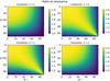 |
Fig. 6. Ratio at resonance of the exact polarization-dependent differential cross-sections (5a)–(5d) to the approximate expressions (6a)–(6d) for different incident and scattered angles θ and θ′, respectively. In all cases, the resonant frequency is given by expression (7) and B = 0.03. |
For quick calculations with B ≪ 1, where high accuracy is not demanded, one may safely use the very simple expressions, given by Eqs. (6a)–(6d), while for more accurate ones, the expressions in Eqs. (5a)–(5d) are recommended. Of course, the highest accuracy is provided by the expressions of Sina (1996). It is our hope that these very simple expressions, together with the prescription that we give in the next subsection, will make resonant Compton scattering calculations more feasible.
2.4. The prescription
If, in a calculation, we want to use the much simpler differential cross-sections (1a)–(1d), then for accurate results, the following prescription should be followed: (1) the spin-flip terms must be added by hand. Thus, Eqs. (6a)–(6d) should be used. Of course, the exact results given by Eqs. (5a)–(5d) are not that complicated; (2) for the resonant frequency, ωr, the relativistically correct expression:
should be used in the Lorentz profile (2) and not the cyclotron frequency ωc = Ec/ℏ.
(3) In the classical (Thomson) limit, there is no change in the photon energy after scattering, namely, ϵ′=ϵ. However, there is naturally an energy change (see Appendix A) and the prescription dictates that the energy ϵ′ of the photon after scattering should be taken equal to:

where

and

If the polarization of the CRSF is not of interest, then the polarization-averaged cross-section can be used, namely:
![$$ \begin{aligned} { {\mathrm{d} \sigma } \over {\mathrm{d} \cos \theta ^\prime } } = 2 \pi { {3 \pi r_0 c} \over 16} (1+\cos ^2 \theta )(1+ \cos ^2 \theta ^\prime )\left[L_{-} + {B \over 2} \cdot L_{+}\right]. \end{aligned} $$](/articles/aa/full_html/2021/11/aa39268-20/aa39268-20-eq32.gif)
We note that for B ≪ 1, the polarization-averaged cross-section in Eq. (3) is very accurate. No additional terms due to spin flip are necessary here.
In this paper, we have restricted ourselves to cyclotron energies of Ec ≲ 50 keV because most of the observed CRSFs are in this energy range (Staubert et al. 2019). However, a few CRSFs with Ec > 50 keV have been observed (Staubert et al. 2019), along with the recently reported (Ge et al. 2020) champion with Ec = 90.32 keV. For this reason, in Fig. 7, we compare the relativistically correct dσ12/d cos θ′(θ = 0, θ′=π/2) of Sina (1996) with the modified classical one (Eq. (6b)) for Ec = 25 keV (left panel), 50 keV (middle panel), and 100 keV (right panel). Clearly, 100 keV is not much less than mec2. Nevertheless, we include it here to demonstrate the magnitude of the discrepancy between classical and quantum-mechanical cross-sections.
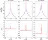 |
Fig. 7. Quantum mechanical differential cross-section versus the classical one for the transition 1 → 2. Top panels: comparison of the relativistically correct dσ12/d cos θ′(θ = 0, θ′=π/2) from Sina (1996) (blue solid line) with the modified classical one (Eq. (6b)) (red dashed line) for Ec = 25 keV (left panel), 50 keV (middle panel), and 100 keV (right panel). Bottom panels: corresponding ratios of the curves shown in the top panels |
3. Summary
In this work, we show numerically that for photon energies, E ≪ mec2, and magnetic field strengths, ℬ ≪ ℬcr, the relativistic polarization-dependent resonant differential cross-sections of Harding & Daugherty (1991), derived with the Johnson & Lippmann (1949) wave functions, are in excellent agreement with those of Sina (1996), which were derived with the (Sokolov & Ternov 1968) formalism.
We show analytically that the expansion up to the first order in ϵ = E/mec2 and B = ℬ/ℬcr of the expressions of Harding & Daugherty (1991) and of Sina (1996) lead to nearly identical results.
We provide simple, heuristic, but very accurate, expressions for the polarization-dependent resonant differential cross-sections, together with a prescription that ought to be followed for easy-to-perform and detailed calculations involving resonant scattering at Ec ≲ 50 keV.
Acknowledgments
We thank the anonymous referee for pointing out to us the Sokolov & Ternov (1968) formalism. We also thank Roberto Turolla and Alexander Mushtukov for useful discussions concerning the Sokolov & Ternov (1968) formalism. We are indebted to Alice Harding for sending us the unpublished PhD Thesis of Ramin Sina and to Peter Gonthier for e-mail exchanges. N.D.K. would like to thank Sterl Phinney for his notes on the classical magnetic scattering cross-sections.
References
- Araya, R., & Harding, A. 1999, ApJ, 517, 334 [NASA ADS] [CrossRef] [Google Scholar]
- Araya-Góchez, R., & Harding, A. 2000, ApJ, 544, 1067 [CrossRef] [Google Scholar]
- Baring, M. G., Gonthier, P. L., & Harding, A. K. 2005, ApJ, 630, 430 [NASA ADS] [CrossRef] [Google Scholar]
- Basko, M. M., & Sunyaev, R. A. 1976, MNRAS, 175, 395 [Google Scholar]
- Blandford, R. D., & Scharleman, E. T. 1976, MNRAS, 174, 59 [NASA ADS] [CrossRef] [Google Scholar]
- Bussard, R. W., Alexander, S. B., & Meszaros, P. 1986, Phys. Rev. D, 34, 440 [NASA ADS] [CrossRef] [Google Scholar]
- Canuto, V., Lodenquai, J., & Ruderman, M. 1971, Phys. Rev. D, 3, 2303 [NASA ADS] [CrossRef] [Google Scholar]
- Daugherty, J. K., & Harding, A. K. 1986, ApJ, 309, 362 [NASA ADS] [CrossRef] [Google Scholar]
- Daugherty, J. K., & Ventura, J. 1978, Phys. Rev. D, 18, 1053 [NASA ADS] [CrossRef] [Google Scholar]
- Ge, M. Y., Ji, L., Zhang, S. N., et al. 2020, ApJ, in press [Google Scholar]
- Gonthier, P. L., Baring, M. G., Eiles, M. T., et al. 2014, Phys. Rev. D, 90, 043014 [NASA ADS] [CrossRef] [Google Scholar]
- Harding, A. K., & Daugherty, J. K. 1991, ApJ, 374, 687 [NASA ADS] [CrossRef] [Google Scholar]
- Herold, H. 1979, Phys. Rev. D, 19, 2868 [NASA ADS] [CrossRef] [Google Scholar]
- Herold, H., Ruder, H., & Wunner, G. 1982, A&A, 115, 90 [NASA ADS] [Google Scholar]
- Johnson, M. H., & Lippmann, B. A. 1949, Phys. Rev., 76, 828 [NASA ADS] [CrossRef] [Google Scholar]
- Mushtukov, A. A., Nagirner, D. I., & Poutanen, J. 2016, Phys. Rev. D, 93, 105003 [Google Scholar]
- Nagel, W. 1981, ApJ, 251, 288 [Google Scholar]
- Nishimura, O. 2008, ApJ, 672, 1127 [NASA ADS] [CrossRef] [Google Scholar]
- Nobili, L., Turolla, R., & Zane, S. 2008a, MNRAS, 389, 989 [NASA ADS] [CrossRef] [Google Scholar]
- Nobili, L., Turolla, R., & Zane, S. 2008b, MNRAS, 386, 1527 [NASA ADS] [CrossRef] [Google Scholar]
- Pavlov, G. G., Bezchastnov, V. G., Meszaros, P., & Alexander, S. G. 1991, ApJ, 380, 541 [NASA ADS] [CrossRef] [Google Scholar]
- Poutanen, J., Mushtukov, A. A., Suleimanov, V. F., et al. 2013, ApJ, 777, 115 [NASA ADS] [CrossRef] [Google Scholar]
- Schönherr, G., Wilms, J., Kretschmar, P., et al. 2007, A&A, 472, 353 [NASA ADS] [CrossRef] [EDP Sciences] [Google Scholar]
- Schwarm, F. W. 2017, PhD Thesis (Erlangen: Friedrich-Alexander Universität) [Google Scholar]
- Sina, R. 1996, PhD Thesis (Maryland: University of Maryland) [Google Scholar]
- Sokolov, A. A., & Ternov, I. M. 1968, Radiation from Relativistic Electrons (Melville, NY: American Institute of Physics) [Google Scholar]
- Staubert, R., Trümper, J. E., Kendziorra, E., et al. 2019, A&A, 622, 61 [Google Scholar]
- Trümper, J., Pietsch, W., Reppin, C., et al. 1977, Ann. N. Y. Acad. Sci, 302, 538 [CrossRef] [Google Scholar]
- Trümper, J., Pietsch, W., Reppin, C., et al. 1978, ApJ, 219, L105 [CrossRef] [Google Scholar]
- Ventura, J. 1979, Phys. Rev. D., 19, 1684 [NASA ADS] [CrossRef] [Google Scholar]
- Ventura, J., Nagel, W., & Meszaros, P. 1979, ApJ, 233, L125 [NASA ADS] [CrossRef] [Google Scholar]
Appendix A: Approximations resulting from the Harding & Daugherty (1991) expressions
We start from Eq. (11) of Harding & Daugherty (1991), which has been derived in the electron’s rest frame, considering that the electron initially occupies the ground state. In a unit system where ℏ = c = me = 1, this equation can be written as follows:
where σT is the Thomson cross-section, ω, ω′ are the incident and scattered photon frequencies in units of mec2/ℏ, whereas θ and θ′ are the incident and scattered photon angles with respect to the magnetic field direction, B is the magnetic field strength ℬ (in units of ℬcr), Φ is proportional to sin(ϕ − ϕ′), and ϕ and ϕ′ are the azimuthal angles of the incident and the scattered photon, respectively. The terms  ,
,  are complex functions of θ, θ′, ω, ω′, B, ϕ, ϕ′, s, s′ and these terms can be found in the appendix of Harding & Daugherty (1991), where the upper indices (1, 2) are referred to the first and second Feynman diagram. Furthermore, s and s′ stand for the incident and scattered photon polarization mode and l is the final electron’s Landau state. We note that the infinite sum in Eq. (A.1) is carried out over intermediate Landau states with principal quantum number, n, whereas the sum over i = 1, 2 is meant for the possible electron spin orientations (spin-up, spin-down) in the intermediate state.
Equation (A.1) is quite general, but this generality is not needed in most cases. Specifically, for resonant scattering of photons with energy E ≲ mec2 in a magnetic field smaller than or comparable to the critical one  , Nobili et al. (2008b, hereafter NTZ08b) pointed out that for such magnetic fields, the probability of exciting Landau levels above the second (n = 2) is very small, thus the infinite sum over n in Eq. (A.1) becomes finite (n ≤ 2).
Moreover, for photon energies, E ≪ mec2, and magnetic fields, ℬ ≪ ℬcr, which we are interested in here, the cross-section expressions can be simplified even more, keeping only the term n = 1 in the sum over all the possible intermediate states and setting l = 0 for the final electron Landau state. Besides that, as NTZ08b stated, the  terms exhibit a divergent behavior near resonant frequency (see their Eqs. (7) and (8)), while the terms
  , remain instead finite. Given this observation, and as long as we are interested in resonant scattering (i.e., photon frequency near the resonant one), the above arguments lead us to a major simplification.
Neglecting all the non-resonant terms and the contributions of (n ≠ 1) in Eq. (A.1), we deduce the following expression:
NTZ08b managed to write the above equation in a simpler way, obtaining compact expressions for the  terms. Specifically, using Eq. (14) of NTZ08b in Eq. (10) of NTZ08b we obtain:
where, for convenience, we retain the notation of NTZ08b; but for simplicity, we drop the indices referring to n = 1 and l = 0. Thus, ϵ, ϵ′ are the incident and scattered photon energies in units of mec2, θ and θ′ are the incident and scattered photon angles with respect to the magnetic field direction, B is the magnetic field strength ℬ (in units of ℬcr). and Γ+, Γ− are the relativistic decay rates corresponding to the n = 1 intermediate state and are given by Herold et al. (1982, see also Harding & Daugherty 1991; Pavlov et al. 1991; Baring et al. 2005; NTZ08b), where the index “+" stands for the electron in the intermediate state with spin-up whereas the index “–" stands for spin-down. In addition, s and s′ refer to the incident and scattered photon polarization modes, and the explicit expressions for the  ,
,  terms are given in the Appendix of NTZ08b for n = 1 and l = 0.
We remark that we do not use the relativistic polarization-dependent resonant Compton differential cross-section expressions of NTZ08b because, for their purposes, the authors substituted all the Lorentz profiles with a δ−function and, as a result, the information about the exact shape of the different line profiles is lost.
The energy, E1, is the electron intermediate state and, in units of mec2, it is given by Eq. (12) of NTZ08b (see also Eq. (4) of Harding & Daugherty 1991).
The energy ϵ′ of the photon after scattering, in units of mec2, is given by Eq. (6) of NTZ08b (see also Eq. (12) of Harding & Daugherty 1991):
where

and

After a lengthy but straightforward calculation, and a trivial integration over the angle ϕ′, one can write Eq. (A.3) in the following way:
![$$ \begin{aligned} {{d\sigma _{ss^\prime }} \over {d\cos \theta ^\prime }}&= { {3\pi \sigma _T} \over {16} } { {(1+E_1)^2} \over {E_1\sqrt{1 + 2B\sin ^2\theta }}} { {\epsilon ^\prime } \over {\epsilon } } A \nonumber \\&\times \left[{ {(T_+^{s \rightarrow s^\prime })^2}\over {\Gamma _{+} }} \mathcal{L}_{+} + { {(T_-^{s \rightarrow s^\prime })^2}\over {\Gamma _{-} }} \mathcal{L}_{-} + 2{{T_+^{s \rightarrow s^\prime }T_-^{s \rightarrow s^\prime }} \over {\Gamma _{\rm mix}} } {{\mathcal{L}_{+}\mathcal{L}_{-}} \over {\mathcal{L}_{\rm mix}}} \right], \end{aligned} $$](/articles/aa/full_html/2021/11/aa39268-20/aa39268-20-eq48.gif)
where the effective decay rates  , which result from the change in the Lorentz profiles argument (see NTZ08b), must be used in the Lorentz profiles (see Eqs. (A.8)–(A.10)):
and we define the following function:
The quantities ℒ+(ϵ,ϵr), ℒ−(ϵ,ϵr) & ℒmix(ϵ,ϵr) are the dimensionless Lorentz profiles and are given by

where  is calculated by
with
and ϵr is the resonant energy in units of mec2. It is given by Eq. (8) of NTZ08b (see also Eq. (5) of Harding & Daugherty 1991):
Having obtained the fully relativistic cross-sections we proceed to the derivation of Eqs. (4a)–(4d).
Expansion up to first order in the small parameters ϵ, ϵ′, and B yields
![$$ \begin{aligned} { {(1+E_1)^2} \over {E_1 \sqrt{1+2B \sin ^2\theta }} }{ {\epsilon ^\prime } \over {\epsilon } } A \approx 8\left[1-B\left(2\sin ^2\theta + (\cos \theta - \cos \theta ^\prime )^2 \right) \right]. \end{aligned} $$](/articles/aa/full_html/2021/11/aa39268-20/aa39268-20-eq60.gif)
To lowest order, Γ+, Γ− are given in Herold et al. (1982) (see also Eqs. (15), (16) of Harding & Daugherty 1991 and Eq. (31) of NTZ08b)

and substituting the above expressions into Eq. (A.11b), we get:
where α is the fine structure constant. For a discussion regarding the cyclotron line widths, see our Appendix C.
We note that the classical cross-sections (1) and the expressions in Eq. (4) are proportional to r0c, while the quantum-mechanical ones are proportional to σT. This means that the Lorentz profiles with variable the photon frequency (i.e. L+(ω, ωr), L−(ω, ωr) and Lmix(ω, ωr)) have dimensions of time and their relation with the dimensionless ones (i.e. ℒ+(ϵ,ϵr), ℒ−(ϵ,ϵr) & ℒmix(ϵ,ϵr)) are (see Appendix C)
where the Lorentz profiles with argument the photon frequency are given by
and
Using the above, we find that Eq. (A.6) is approximated by the following:
![$$ \begin{aligned} \dfrac{d\sigma _{ss^\prime }}{d\cos \theta ^\prime }&\approx \dfrac{3\pi \sigma _T}{2}\dfrac{m_{\rm e}c^2}{{\hbar }} W(B, \theta , \theta ^\prime ) \nonumber \\&\times \left[{ {(T_+^{s \rightarrow s^\prime })^2}\over {\Gamma _{+} }} L_{+} + { {(T_-^{s \rightarrow s^\prime })^2}\over {\Gamma _{-} }} L_{-} + 2{{T_+^{s \rightarrow s^\prime }T_-^{s \rightarrow s^\prime }} \over {\Gamma _{\rm mix}} } {{L_{+} L_{-}} \over {L_{\rm mix}}} \right], \nonumber \\&= 2\pi \dfrac{3\pi r_o c}{8}\left(\dfrac{16 \alpha }{3}\right) W(B, \theta , \theta ^\prime ) \nonumber \\&\times \left[{ {(T_+^{s \rightarrow s^\prime })^2}\over {\Gamma _{+} }} L_{+} + { {(T_-^{s \rightarrow s^\prime })^2}\over {\Gamma _{-} }} L_{-} + 2{{T_+^{s \rightarrow s^\prime }T_-^{s \rightarrow s^\prime }} \over {\Gamma _{\rm mix}} } {{L_{+} L_{-}} \over {L_{\rm mix}}} \right], \end{aligned} $$](/articles/aa/full_html/2021/11/aa39268-20/aa39268-20-eq73.gif)
where

and using:

The expressions for  and
and  have strong polarization dependence and, as we mentioned earlier, are given in the Appendix of NTZ08b. In order to obtain Eq. (4), we will work separately for each pair, s, s′.
A.1. Transition 1 → 1
By expanding the terms  ,
,  in the small parameters ϵ, ϵ′, and B, and employing Eqs. (A.15) and (A.21), we obtain the following approximations:
![$$ \begin{aligned} \dfrac{(T^{1 \rightarrow 1}_-)^2}{\Gamma _-}&\approx \dfrac{3}{16\alpha } \cos ^2\theta \cos ^2\theta ^\prime \nonumber \\&\times \bigg [1 - B\left(2 + \sin ^2\theta + \dfrac{2\sin ^2\theta ^\prime \cos \theta }{\cos \theta ^\prime } - \sin ^2\theta ^\prime \right)\bigg ] , \end{aligned} $$](/articles/aa/full_html/2021/11/aa39268-20/aa39268-20-eq81.gif)

Equations (A.22), along with (A.19), lead us to derive the following approximation for dσ11/d cos θ′
![$$ \begin{aligned} { {d \sigma _{11}} \over {d\cos \theta ^\prime } }&\approx 2\pi { {3\pi r_o c} \over {8} }\Big [ g^{1 \rightarrow 1} \cdot L_{-} + h^{1 \rightarrow 1} \cdot L_{+}\nonumber \\&+ \sqrt{2B}\cos \theta \cos \theta ^\prime \dfrac{L_{-} \cdot L_{+}}{L_{\rm mix}} \Big ], \end{aligned} $$](/articles/aa/full_html/2021/11/aa39268-20/aa39268-20-eq83.gif)
where
![$$ \begin{aligned} g^{1 \rightarrow 1}(\theta ,\theta ^\prime , B)&=\cos ^2\theta \cos ^2\theta ^\prime \bigg [1 - B\bigg (3\sin ^2\theta - \sin ^2\theta ^\prime \nonumber \\&+ (\cos \theta - \cos \theta ^\prime )^2 + 2 + 2\sin ^2\theta ^\prime \dfrac{\cos \theta }{\cos \theta ^\prime } \bigg )\bigg ], \end{aligned} $$](/articles/aa/full_html/2021/11/aa39268-20/aa39268-20-eq84.gif)
and
A.2. Transition 1 → 2
We apply the same methodology to all the other cases. Hence, by expanding the terms  ,
,  in the small parameters ϵ, ϵ′, and B, and using Eqs. (A.15) and (A.21), we find the following approximations:
![$$ \begin{aligned} \dfrac{(T^{1 \rightarrow 2}_-)^2}{\Gamma _-} \approx \dfrac{3}{16\alpha } \cos ^2\theta \left[1 - B\left(2 + \sin ^2\theta \right)\right] , \end{aligned} $$](/articles/aa/full_html/2021/11/aa39268-20/aa39268-20-eq89.gif)

Then, by substituting Eqs. (A.24) into (A.19), we get the following approximation:
![$$ \begin{aligned} { {d \sigma _{12}} \over {d\cos \theta ^\prime } }&\approx 2\pi { {3\pi r_o c} \over {8} }\Big [g^{1 \rightarrow 2} \cdot L_{-} + h^{1 \rightarrow 2} \cdot L_{+} \nonumber \\&+ \sqrt{2B}\cos \theta \cos \theta ^\prime \dfrac{L_{-} \cdot L_{+}}{L_{\rm mix}} \Big ], \end{aligned} $$](/articles/aa/full_html/2021/11/aa39268-20/aa39268-20-eq91.gif)
where
![$$ \begin{aligned} g^{1 \rightarrow 2}(\theta ,\theta ^\prime ,B)&=\cos ^2\theta \bigg [1 - B\bigg (3\sin ^2\theta + 2 \nonumber \\&+ (\cos \theta - \cos \theta ^\prime )^2 \bigg )\bigg ], \end{aligned} $$](/articles/aa/full_html/2021/11/aa39268-20/aa39268-20-eq92.gif)
and
A.3. Transition 2 → 1
Similarly, by expanding the terms  ,
,  in the small parameters ϵ, ϵ′, and B, and taking into account Eqs. (A.15) and (A.21), we can deduce the following approximations:
![$$ \begin{aligned} \dfrac{(T^{2 \rightarrow 1}_-)^2}{\Gamma _-}&\approx \dfrac{3}{16\alpha } \cos ^2\theta ^\prime \nonumber \\&\times \bigg [1 - B\left(2 - \sin ^2\theta ^\prime + 2\sin ^2\theta ^\prime \dfrac{\cos \theta }{\cos \theta ^\prime } \right)\bigg ], \end{aligned} $$](/articles/aa/full_html/2021/11/aa39268-20/aa39268-20-eq97.gif)
Using Eqs. (A.26) and (A.19), we find
![$$ \begin{aligned} { {d \sigma _{21}} \over {d\cos \theta ^\prime } }&\approx 2\pi { {3\pi r_o c} \over {8} }\Big [ g^{2 \rightarrow 1} \cdot L_{-} + h^{2 \rightarrow 1} \cdot L_{+} \nonumber \\&+ \sqrt{2B}\cos \theta \cos \theta ^\prime \dfrac{L_{-} \cdot L_{+}}{L_{\rm mix}} \Big ], \end{aligned} $$](/articles/aa/full_html/2021/11/aa39268-20/aa39268-20-eq99.gif)
where
![$$ \begin{aligned} g^{2 \rightarrow 1}(\theta ,\theta ^\prime ,B)&=\cos ^2\theta ^\prime \bigg [1 - B \bigg (2\sin ^2\theta + (\cos \theta - \cos \theta ^\prime )^2\nonumber \\&+ 2 - \sin ^2\theta ^\prime + 2\sin ^2\theta ^\prime \dfrac{\cos \theta }{\cos \theta ^\prime } \bigg )\bigg ], \end{aligned} $$](/articles/aa/full_html/2021/11/aa39268-20/aa39268-20-eq100.gif)
and
A.4. Transition 2 → 2
Following the same procedure as above, for the terms  ,
,  and employing Eqs. (A.15) and (A.21), we derive the following:

Thus, the substitution of Eqs. (A.28) into (A.19) yields
![$$ \begin{aligned} { {d \sigma _{22}} \over {d\cos \theta ^\prime } }&\approx 2\pi { {3\pi r_o c} \over {8} }\Big [ g^{2 \rightarrow 2} \cdot L_{-} + h^{2 \rightarrow 2} \cdot L_{+}\nonumber \\&+ \sqrt{2B}\cos \theta \cos \theta ^\prime \dfrac{L_{-} \cdot L_{+}}{L_{\rm mix}} \Big ], \end{aligned} $$](/articles/aa/full_html/2021/11/aa39268-20/aa39268-20-eq107.gif)
where
![$$ \begin{aligned} g^{2 \rightarrow 2}(\theta ,\theta ^\prime ,B)=1 - B\left[2\sin ^2\theta + (\cos \theta - \cos \theta ^\prime )^2 + 2 \right], \end{aligned} $$](/articles/aa/full_html/2021/11/aa39268-20/aa39268-20-eq108.gif)
and
Appendix B: Approximations resulting from the Sina (1996) expressions
We start from Eq. (3.25) of Sina (1996), written in the electron’s rest frame (ground state), considering a unit system where ℏ = me = c = 1, (i.e., energy is measured in mec2, frequency is measured in mec2/ℏ and the magnetic field strength, ℬ, is measured in ℬcr = e−1). We neglect any terms that are related to the second Feynman diagram, as well as the terms that the intermediate electron Landau state has a principal quantum number n ≠ 1 (i.e., keeping only the terms that exhibit a divergence near resonant frequency with n = 1, as we did in Appendix A). Thus, the infinite sum over n for all possible intermediate states collapses to the following:
where Zc1(n = 1) is given by Eq. (3.15) of Sina (1996) and is a sum over the possible electron spin orientations, sn, in the intermediate state (for spin-up sn = +1, whereas for spin-down sn = −1):
We retain the notation of Sina (1996), thus ωi is the incident photon frequency, Ei is the electron’s energy before scattering, θi, θf are the incident and scattered photon angles with respect to the magnetic field direction, whereas the indices i and f stand for the initial and final electron Landau states (in our case, they are equal to 0, i.e., the ground state), the si and sf are the initial and final electron’s spin orientations and are equal to -1 (since only spin-down is allowed in the ground state), and ki, kf are the incident and scattered electron wavenumbers, respectively. Furthermore, En = 1, 1 (E1, hereafter) is the electron’s energy in the intermediate state with n = 1 and is given by Eq. (3.3) of Sina (1996) (see also Eq. (3.1) of Schwarm 2017):
where a misprint has been corrected and we substituted Eq. (3.4) of Sina (1996) into Eq. (3.3) of Sina (1996) and took into account that the initial electron momentum pi is equal to zero, since we are working in the electron’s rest frame. Moreover, βf can be written as pf/Ef (see Eq. (B.18) of Gonthier et al. 2014), where Ef and pf are the final electron energy and parallel component of momentum (with respect to the magnetic field direction) and are calculated by imposing the conservation of energy and by Eq. (3.29) of Sina (1996). Thus
and

We note that ωf is the scattered photon frequency and is given by Eq. (3.28) of Sina (1996), although it is actually our Eq. (A.5) written in a different form, so we do not present it here and  ,
,  (Γ+, Γ−, hereafter) are the relativistic decay widths for the electron in the intermediate state with spin-up and spin-down, respectively, and are given by Herold et al. (1982). Figure 3.4 of Schwarm (2017) verifies that the decay widths of Sina (1996) are in full agreement with the ones of Herold et al. (1982), which we have used in Appendix A. This is reasonable and absolutely predictable, since both works have employed electron wave functions of Sokolov & Ternov (1968).
Substituting the above into Eq. (B.1) and using that the initial electron energy, E1, is equal to 1 and α2 = 3σT/8π in this system of units, we obtain
where the complex functions Df, n, sf, sn(kf) and Hn, i, sn, si(ki) have a strong polarization dependence, since they depend on the polarization modes of the incident and scattered photons; these are given in Appendix D of Sina (1996). Specifically, the Df, n, sf, sn(kf) terms exclusively depend on the final photon polarization mode and are calculated by Eqs. (D.61), (D.66) of Sina (1996)
![$$ \begin{aligned}&D_{\perp }^{f=0,n=1,s_f=-1,s_n}(k_f)=\nonumber \\&i\bigg [\big (C_{1,f=0}C_{4,n=1} + C_{3,f=0}C_{2,n=1}\big )\Lambda _{-1,1}(k_f) -\nonumber \\&\big (C_{2,f=0}C_{3,n=1} + C_{4,f=0}C_{1,n=1}\big )\Lambda _{0,0}(k_f)\bigg ], \end{aligned} $$](/articles/aa/full_html/2021/11/aa39268-20/aa39268-20-eq118.gif)
![$$ \begin{aligned}&D_{\parallel }^{f=0,n=1,s_f=-1,s_n}(k_f)=\nonumber \\&\cos \theta _f\bigg [\big (C_{1,f=0}C_{4,n=1} + C_{3,f=0}C_{2,n=1}\big )\Lambda _{-1,1}(k_f) +\nonumber \\&\big (C_{2,f=0}C_{3,n=1} + C_{4,f=0}C_{1,n=1}\big )\Lambda _{0,0}(k_f)\bigg ] -\nonumber \\&\sin \theta _f\bigg [\big (C_{1,f=0}C_{3,n=1} + C_{3,f=0}C_{1,n=1}\big )\Lambda _{-1,0}(k_f) -\nonumber \\&\big (C_{2,f=0}C_{4,n=1} + C_{4,f=0}C_{2,n=1}\big )\Lambda _{0,1}(k_f)\bigg ], \end{aligned} $$](/articles/aa/full_html/2021/11/aa39268-20/aa39268-20-eq119.gif)
while the terms Hn, i, sn, si(ki) exclusively depend on the initial photon polarization mode and are given by Eqs. (D.60), (D.65) of Sina (1996):
![$$ \begin{aligned}&H_{\perp }^{n=1,i=0,s_n,s_i=-1}(k_i)=\nonumber \\&i\bigg [\big (C_{1,n=1}C_{4,i=0} + C_{3,n=1}C_{2,i=0}\big )\Lambda _{0,0}(k_i) -\nonumber \\&\big (C_{2,n=1}C_{3,i=0} + C_{4,n=1}C_{1,i=0}\big )\Lambda _{-1,1}(k_i)\bigg ], \end{aligned} $$](/articles/aa/full_html/2021/11/aa39268-20/aa39268-20-eq120.gif)
![$$ \begin{aligned}&H_{\parallel }^{n=1,i=0,s_n,s_i=-1}(k_i)=\nonumber \\&\cos \theta _i\bigg [\big (C_{1,n=1}C_{4,i=0} + C_{3,n=1}C_{2,i=0}\big )\Lambda _{0,0}(k_i) +\nonumber \\&\big (C_{2,n=1}C_{3,i=0} + C_{4,n=1}C_{1,i=0}\big )\Lambda _{-1,1}(k_i)\bigg ] -\nonumber \\&\sin \theta _i\bigg [\big (C_{1,n=1}C_{3,i=0} + C_{3,n=1}C_{1,i=0}\big )\Lambda _{-1,0}(k_i) -\nonumber \\&\big (C_{2,n=1}C_{4,i=0} + C_{4,n=1}C_{2,i=0}\big )\Lambda _{0,1}(k_i)\bigg ], \end{aligned} $$](/articles/aa/full_html/2021/11/aa39268-20/aa39268-20-eq121.gif)
where the lower index “∥” stands for the ordinary polarization mode and the lower index “⊥” stands for the extraordinary polarization mode. Moreover, the quantities Ck with k = 1, 2, 3, 4, are the wave function coefficients of Sokolov & Ternov (1968) and are given by Eqs. (B.61)–(B.65) of Sina (1996), whereas the Λi, j functions are proportional to Laguerre polynomials and are given in Appendix D of Sina (1996). We note that we can also obtain all of the above using Appendix B of Gonthier et al. (2014).
After a lengthy, but straightforward calculation, we can write Eq. (B.4) in the following form:
![$$ \begin{aligned} \dfrac{d\sigma _{ss^\prime }}{d \cos \theta _f}&= \dfrac{3\pi \sigma _T}{2} \dfrac{E_1}{\sqrt{1 + 2B\sin ^2\theta _i}}\dfrac{\omega _f}{\omega _i} \mathcal{A}\nonumber \\&\times \left[{ {\mathcal{T}_+^{s \rightarrow s^\prime }}\over {\Gamma _{+} }} \mathcal{L}_{+} + { {\mathcal{T}_-^{s \rightarrow s^\prime }}\over {\Gamma _{-} }} \mathcal{L}_{-} + 2{{\mathcal{T}_{\rm mix}^{s \rightarrow s^\prime }} \over {\Gamma _{\rm mix}} } {{\mathcal{L}_{+}\mathcal{L}_{-}} \over {\mathcal{L}_{\rm mix}}} \right], \end{aligned} $$](/articles/aa/full_html/2021/11/aa39268-20/aa39268-20-eq122.gif)
where we carried out a trivial integration over the scattered photon azimuthal angle, ϕf. Also, for simplicity, we have defined the following quantities
![$$ \begin{aligned} 2\mathcal{T}_{\rm mix}^{s \rightarrow s^\prime }&=\exp ((\omega ^2_i\sin ^2\theta _i + \omega ^2_f\sin ^2\theta _f)/2B)\nonumber \\&\times \bigg [\bigg ((D_{s^\prime }^{f=0,n=1,s_f=-1,s_n=+1}H_{s}^{n=1,i=0,s_n=+1,s_i=-1}\big )^{*}\nonumber \\&\times D_{s^\prime }^{f=0,n=1,s_f=-1,s_n=-1}H_{s}^{n=1,i=0,s_n=-1,s_i=-1} \bigg ) +\nonumber \\&\bigg (D_{s^\prime }^{f=0,n=1,s_f=-1,s_n=+1}H_{s}^{n=1,i=0,s_n=+1,s_i=-1}\nonumber \\&\times \big (D_{s^\prime }^{f=0,n=1,s_f=-1,s_n=-1}H_{s}^{n=1,i=0,s_n=-1,s_i=-1} \big )^{*}\bigg ) \bigg ]. \end{aligned} $$](/articles/aa/full_html/2021/11/aa39268-20/aa39268-20-eq126.gif)
We note that the dimensionless Lorentz profiles ℒ+(ωi,ωr), ℒ−(ωi,ωr), and ℒmix(ωi,ωr) that are shown in Eq. (B.7a) are the same as the ones in Appendix A, since in this unit system, the dimensionless photon frequencies, ωi, ωf, and the dimensionless resonant frequency have the same values with the corresponding dimensionless energies and, as we mentioned earlier in this paper, the decay widths are identical to those shown in Appendix A (and so are the effective decay widths given by Eqs. (A.7a), (A.11b)). Furthermore, the dimensionless resonant frequency, ωr, is given by Eq. (5) of Harding & Daugherty (1991) and is actually the same as the dimensionless resonant energy (Eq. (A.12))
Having obtained Eq. (B.7), we are able to proceed to the derivation of Eqs. (5a)–(5d). Expansion up to first order in the small parameters ωi, ωf, and B yields:


Using the above, we find that Eq. (B.7a) can be approximated by
![$$ \begin{aligned} \dfrac{d\sigma _{ss^\prime }}{d \cos \theta _f}&\approx \dfrac{3\pi \sigma _T}{2}\mathcal{W}(\theta _i,\theta _f,B)\nonumber \\&\times \left[{ {\mathcal{T}_+^{s \rightarrow s^\prime }}\over {\Gamma _{+} }} \mathcal{L}_{+} + { {\mathcal{T}_-^{s \rightarrow s^\prime }}\over {\Gamma _{-} }} \mathcal{L}_{-} + 2{{\mathcal{T}_{\rm mix}^{s \rightarrow s^\prime }} \over {\Gamma _{\rm mix}} } {{\mathcal{L}_{+}\mathcal{L}_{-}} \over {\mathcal{L}_{\rm mix}}} \right], \end{aligned} $$](/articles/aa/full_html/2021/11/aa39268-20/aa39268-20-eq131.gif)
and recalling the dimensions of each quantity by taking into account the procedure as well as the results of Appendix A, we obtain the following approximation
![$$ \begin{aligned} \dfrac{d\sigma _{ss^\prime }}{d\cos \theta _f}&\approx 2\pi \dfrac{3\pi r_o c}{8}\left(\dfrac{16 \alpha }{3}\right) \mathcal{W}(\theta _i,\theta _f,B) \nonumber \\&\times \left[{ {\mathcal{T}_+^{s \rightarrow s^\prime }}\over {\Gamma _{+} }} L_{+} + { {\mathcal{T}_-^{s \rightarrow s^\prime }}\over {\Gamma _{-} }} L_{-} + 2{{\mathcal{T}_{\rm mix}^{s \rightarrow s^\prime }} \over {\Gamma _{\rm mix}}} {{L_{+} L_{-}} \over {L_{\rm mix}}} \right], \end{aligned} $$](/articles/aa/full_html/2021/11/aa39268-20/aa39268-20-eq132.gif)
where

From now on, all the quantities have their physical dimensions and, as a result, the Lorentz profiles that are shown in Eq. (B.13a) have dimensions of time and are calculated by Eq. (A.17), where, in the notation that we use in this appendix, the arguments of L+(ωi, ωr), Li(ωi, ωr), and Lmix(ωi, ωr) are ωi and ωr. As we said earlier, the terms  ,
,  , and
, and  have a strong polarization dependence and for this reason, we derive the approximations separately for each possible combination of the incident and scattered photon polarization modes.
B.1. Transition 1 → 1
By expanding the terms  ,
,  , and
, and  in the small parameters ωi, ωf, and B, and employing Eqs. (A.15) and (B.11), we obtain the following approximations:
![$$ \begin{aligned} \dfrac{\mathcal{T}_{-}^{1 \rightarrow 1}}{\Gamma _-}&\approx \dfrac{3}{16\alpha } \cos ^2\theta _i\cos ^2\theta _f\nonumber \\&\times \bigg [1 - B\left(\sin ^2\theta _i + \dfrac{2\sin ^2\theta _f\cos \theta _i}{\cos \theta _f} - \sin ^2\theta _f \right)\bigg ] , \end{aligned} $$](/articles/aa/full_html/2021/11/aa39268-20/aa39268-20-eq141.gif)

Equations (B.14), along with (B.13), lead us to derive the following approximation for dσ11/d cos θf:
![$$ \begin{aligned} { {d \sigma _{11}} \over {d\cos \theta _f} }&\approx 2\pi { {3\pi r_o c} \over {8} }\Big [ \mathcal{G}^{1 \rightarrow 1} \cdot L_{-} + h^{1 \rightarrow 1} \cdot L_{+}\nonumber \\&+ \sqrt{2B}\cos \theta _i\cos \theta _f \dfrac{L_{-} \cdot L_{+}}{L_{\rm mix}} \Big ], \end{aligned} $$](/articles/aa/full_html/2021/11/aa39268-20/aa39268-20-eq143.gif)
where
![$$ \begin{aligned} \mathcal{G}^{1 \rightarrow 1}(\theta _i,\theta _f,B)&=\cos ^2\theta _i \cos ^2\theta _f\bigg [1 - B\bigg (3\sin ^2\theta _i - \sin ^2\theta _f \nonumber \\&+ (\cos \theta _i - \cos \theta _f)^2 -1 + 2\sin ^2\theta _f\dfrac{\cos \theta _i}{\cos \theta _f} \bigg )\bigg ], \end{aligned} $$](/articles/aa/full_html/2021/11/aa39268-20/aa39268-20-eq144.gif)
and

B.2. Transition 1 → 2
We apply the same methodology to all the other cases. Hence, by expanding the terms  ,
,  , and
, and  in the small parameters ωi, ωf, and B, and employing Eqs. (A.15) and (B.11), we find the following approximations

Then, by substituting Eqs. (B.16) into (B.13a), we get the following approximation
![$$ \begin{aligned} { {d \sigma _{12}} \over {d\cos \theta _f} }&\approx 2\pi { {3\pi r_o c} \over {8} }\Big [ \mathcal{G}^{1 \rightarrow 2} \cdot L_{-} + h^{1 \rightarrow 2} \cdot L_{+} \nonumber \\&+ \sqrt{2B}\cos \theta _i\cos \theta _f \dfrac{L_{-} \cdot L_{+}}{L_{\rm mix}} \Big ], \end{aligned} $$](/articles/aa/full_html/2021/11/aa39268-20/aa39268-20-eq152.gif)
where
![$$ \begin{aligned} {\mathcal{G} }^{1 \rightarrow 2}(\theta _{i}, \theta _{f},B)&=\cos ^{2}\theta _{i} \bigg [1 - B\bigg (3\sin ^{2}\theta _{i} -1 \nonumber \\&+ (\cos \theta _{i} - \cos \theta _{f})^{2} \bigg )\bigg ], \end{aligned} $$](/articles/aa/full_html/2021/11/aa39268-20/aa39268-20-eq153.gif)
and
B.3. Transition 2 → 1
Similarly, by expanding the terms  ,
,  , and
, and  in the small parameters ωi, ωf, and B, and taking into account Eqs. (A.15) and (B.11), we can deduce the following approximations:
![$$ \begin{aligned} \dfrac{\mathcal{T}_{-}^{2 \rightarrow 1}}{\Gamma _-}&\approx \dfrac{3}{16\alpha } \cos ^2\theta _f\nonumber \\&\times \bigg [1 - B\left( 2\sin ^2\theta _f\dfrac{\cos \theta _i}{\cos \theta _f}- \sin ^2\theta _f \right)\bigg ], \end{aligned} $$](/articles/aa/full_html/2021/11/aa39268-20/aa39268-20-eq159.gif)

Using Eqs. (B.18) and (B.13a), we find:
![$$ \begin{aligned} { {d \sigma _{21}} \over {d\cos \theta _f} }&\approx 2\pi { {3\pi r_o c} \over {8} }\Big [ \mathcal{G}^{2 \rightarrow 1} \cdot L_{-} + h^{2 \rightarrow 1} \cdot L_{+} \nonumber \\&+ \sqrt{2B}\cos \theta _i\cos \theta _f \dfrac{L_{-} \cdot L_{+}}{L_{\rm mix}} \Big ], \end{aligned} $$](/articles/aa/full_html/2021/11/aa39268-20/aa39268-20-eq161.gif)
where
![$$ \begin{aligned} \mathcal{G}^{2 \rightarrow 1}(\theta _i,\theta _f,B)&=\cos ^2\theta _f\bigg [1 - B \bigg (2\sin ^2\theta _i + (\cos \theta _i - \cos \theta _f)^2 \nonumber \\&-1 - \sin ^2\theta _f + 2\sin ^2\theta _f\dfrac{\cos \theta _i}{\cos \theta _f} \bigg )\bigg ], \end{aligned} $$](/articles/aa/full_html/2021/11/aa39268-20/aa39268-20-eq162.gif)
and
B.4. Transition 2 → 2
Following the same procedure as above for the terms  ,
,  , and
, and  and employing Eqs. (A.15) and (B.11), we can derive:

Thus, the substitution of Eqs. (B.20) into (B.13a), yields
![$$ \begin{aligned} { {d \sigma _{22}} \over {d\cos \theta _f} }&\approx 2\pi { {3\pi r_o c} \over {8} }\Big [ \mathcal{G}^{2 \rightarrow 2} \cdot L_{-} + h^{2 \rightarrow 2} \cdot L_{+} \nonumber \\&+ \sqrt{2B}\cos \theta _i\cos \theta _f \dfrac{L_{-} \cdot L_{+}}{L_{\rm mix}} \Big ], \end{aligned} $$](/articles/aa/full_html/2021/11/aa39268-20/aa39268-20-eq170.gif)
where
![$$ \begin{aligned} \mathcal{G}^{2 \rightarrow 2}(\theta _i,\theta _f,B)=1 - B\left[2\sin ^2\theta _i + (\cos \theta _i - \cos \theta _f)^2 - 1 \right], \end{aligned} $$](/articles/aa/full_html/2021/11/aa39268-20/aa39268-20-eq171.gif)
and
Appendix C: Cyclotron line widths
The spin-dependent relativistic cyclotron widths Γ+, Γ− for the transitions from the first excited intermediate electron state to the fundamental n = 0 Landau state are given by Eq. (17) of Herold et al. (1982) and by Eq. (3) of Pavlov et al. (1991). Thus, we do not present the complete formulae here.
From the literature, we know the non-relativistic cyclotron line widths, which consist of the dominant terms and are valid for small magnetic fields (ℬ ≪ ℬcr) (see Herold et al. 1982; NTZ08b).

For greater accuracy, we provide below the next-order corrections in B. These corrections have been derived from numerical fits to the relativistic transition rates of Herold et al. (1982).
In Fig. C.1, we display the relativistic decay rates of Herold et al. (1982), along with the non-relativistic ones and the expressions C.2, which have a first order correction in B.
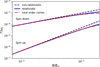 |
Fig. C.1. Comparison of the relativistic transition rates of Herold et al. (1982) (blue solid lines) with the non-relativistic ones (Eq. A.15; black dashed lines) and with the expressions given by Eq. (C.2) (red dash-dotted lines). Spin up refers to spin parallel to the magnetic field, whereas spin down refers to anti-parallel spin. The Γ’s are divided by the cyclotron frequency, ωc, for presentation reasons. |
Clearly, the non-relativistic expressions given in Eq. (C.1) can be used in the Lorentz profiles (defined by Eq. A.17) in the case where B ≪ 1.
All Figures
|
Fig. 1. Polarization-dependent differential cross-section (1/σT) dσ11/d cos θ′ as a function of photon energy E = ℏω for a set of incident angles θ and scattered angles θ′. The set of angles is 0, 30, 60, and 90 degrees, with θ changing vertically and θ′ horizontally. The red solid lines are produced from the expression of Sina (1996), while the black dashed ones are produced from the expression of Harding & Daugherty (1991). In all cases, the resonant frequency is given by expression (7). The vertical line indicates the resonant frequency ωr, which for θ ≠ 0 is smaller than ωc. Here, Ec = ℏωc = 15.33 keV. |
| In the text | |
|
Fig. 2. Ratio of the Harding & Daugherty (1991) polarization-dependent differential cross-section (1/σT) dσ11/d cos θ′ to that of Sina (1996) for the cases shown in Fig. 1. |
| In the text | |
|
Fig. 3. Ratio of the Harding & Daugherty (1991) polarization-dependent differential cross-sections at resonance to those of Sina (1996) for different incident and scattered angles θ and θ′, respectively. In all cases, the resonant frequency is given by Eq. (7) and B = 0.03. |
| In the text | |
|
Fig. 4. Polarization-dependent resonant differential cross-section (1/σT) dσ12/d cos θ′ as a function of photon energy E = ℏω for a set of incident angles θ and scattered angles θ′. The set of angles is 0, 30, 60, and 90 degrees, with θ changing vertically and θ′ horizontally. The red solid lines are produced from the first order expansion (5b) of Sina (1996), while the black dashed ones are produced from the simplified expression (6b). In all cases, the resonant frequency is given by Eq. (7). The vertical line indicates the resonant frequency ωr, which for θ ≠ 0 is smaller than ωc. Here, Ec = ℏωc = 15.33 keV. |
| In the text | |
|
Fig. 5. Ratio of the polarization-dependent differential cross-sections dσ12/d cos θ′ given by (5b) to the simplified expression (6b) for the cases shown in Fig. 4. |
| In the text | |
|
Fig. 6. Ratio at resonance of the exact polarization-dependent differential cross-sections (5a)–(5d) to the approximate expressions (6a)–(6d) for different incident and scattered angles θ and θ′, respectively. In all cases, the resonant frequency is given by expression (7) and B = 0.03. |
| In the text | |
|
Fig. 7. Quantum mechanical differential cross-section versus the classical one for the transition 1 → 2. Top panels: comparison of the relativistically correct dσ12/d cos θ′(θ = 0, θ′=π/2) from Sina (1996) (blue solid line) with the modified classical one (Eq. (6b)) (red dashed line) for Ec = 25 keV (left panel), 50 keV (middle panel), and 100 keV (right panel). Bottom panels: corresponding ratios of the curves shown in the top panels |
| In the text | |
|
Fig. C.1. Comparison of the relativistic transition rates of Herold et al. (1982) (blue solid lines) with the non-relativistic ones (Eq. A.15; black dashed lines) and with the expressions given by Eq. (C.2) (red dash-dotted lines). Spin up refers to spin parallel to the magnetic field, whereas spin down refers to anti-parallel spin. The Γ’s are divided by the cyclotron frequency, ωc, for presentation reasons. |
| In the text | |
Current usage metrics show cumulative count of Article Views (full-text article views including HTML views, PDF and ePub downloads, according to the available data) and Abstracts Views on Vision4Press platform.
Data correspond to usage on the plateform after 2015. The current usage metrics is available 48-96 hours after online publication and is updated daily on week days.
Initial download of the metrics may take a while.