© ESO 2021

1. Introduction

Relativistic hydrodynamics is one of the most successful tools to describe complex dynamical phenomena ranging from cosmological scales to those of colliding particles. General relativity is thereby a necessary ingredient to understand systems with strong gravitational fields, such as accretion discs and the launch of jets in active galactic nuclei (e.g. Mościbrodzka et al. 2014, 2016; Komissarov & Porth 2021) or the mergers of compact objects producing gravitational waves (e.g. Siegel & Metzger 2018). Many other phenomena, however, do not involve strongly bent spacetime but still flow velocities near the speed of light, for example gamma-ray bursts (e.g. Willingale & Mészáros 2017; Zhang 2018), systems with pulsar winds (e.g. Barkov et al. 2019), such as gamma-ray binaries (e.g. Huber et al. 2021a,b) and pulsar wind nebulae (e.g. Olmi & Bucciantini 2019), or interacting heavy-ion beams in collider experiments (e.g. Busza et al. 2018). Their dynamics can therefore be more suitably described in special relativistic frameworks, which we focus on in this work.

Due to the high complexity of many problems in current research, analytical approaches are no longer feasible to explain observed data. Numerical approaches (see Martí & Müller 2003, 2015, for a review) are therefore essential to further our understanding of the related systems. For this, many modern codes have been presented that treat the equations of special relativistic hydrodynamics (SRHD) and/or magnetohydrodynamics (SRMHD), such as PLUTO (Mignone et al. 2007, 2012), RAMSES (Teyssier 2002; Lamberts et al. 2013), ATHENA++ (Stone et al. 2008; White et al. 2016), AMRVAC (Meliani et al. 2007), and others.

In this paper, we present the special relativistic extension of CRONOS (Kissmann et al. 2018), which was used in comprehensive models for the emission of gamma-ray binaries (see Huber et al. 2021a,b). CRONOS is a finite-volume, Godunov-type code that was developed to solve hyperbolic systems of partial differential equations with astrophysical applications in mind. A key feature of CRONOS consists in its easy adaptability and extensibility, providing a framework with several interfaces for customisations by the user that allows for the straightforward incorporation of additional physics, such as the transport of energetic particles (see e.g. Reitberger et al. 2017), radiative cooling of the plasma (see e.g. Scherer et al. 2020), or the use of more general reference frames (see e.g. Huber et al. 2021a). Here we describe the extension of CRONOS to SRHD, where we did not introduce any new algorithms, but selected and combined different techniques that have been proven successful in literature.

The paper is structured as follows: in Sect. 2 we introduce the governing equations; the notations and general structure of the code are defined in Sect. 3; in Sect. 4 we describe the numerical scheme implemented in CRONOS; and we validate it on an extensive set of numerical tests in Sect. 5. Finally, we comment on the parallel performance of the code in Sect. 6 and give a summary in Sect. 7.

2. System of equations

The CRONOS code (Kissmann et al. 2018) was in general developed to solve a set of hyperbolic conservation laws of the form

$$\begin{array}{c}\hfill {\partial }_{t}U+\mathrm{\nabla }·\mathit{F}\left(U\right)=S,\end{array}$$(1)

where U denotes a set of conserved quantities, F the respective fluxes, and S an additional source term.

2.1. Special relativistic hydrodynamics

In analogy to classical hydrodynamics, the dynamics of a relativistic fluid can be expressed as such a system (Landau & Lifshitz 1959). The respective equations for the conservation of rest-mass, energy, and momentum read as follows:

$$\begin{array}{cc}& {\partial }_{t}D+\mathrm{\nabla }·\left(D\mathit{v}\right)=S_D,\hfill \end{array}$$(2a)

$$\begin{array}{cc}& {\partial }_t\tau +\mathrm{\nabla }·((\tau +p)\mathit{v})=S_{\tau },\hfill \end{array}$$(2b)

$$\begin{array}{cc}& {\partial }_t\mathit{m}+\mathrm{\nabla }·(\mathit{m}\otimes \mathit{v}+p\mathbb{1})={\mathit{S}}_{\mathrm{m}},\hfill \end{array}$$(2c)

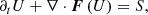
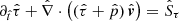
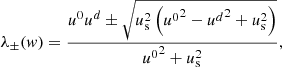
where U = (D, τ, m^j) correspond to the conserved variables, that are the mass, energy, and momentum density in the jth coordinate direction, respectively, and S = (S_D, S_τ, S_m^j) correspond to their respective source terms. The fluxes further involve the fluid’s three-velocity v and pressure p. All quantities are given in the laboratory frame and in natural units, that is with the speed of light c = 1.

It should be noted that the momentum fluxes in Eq. (2c) are given by the rank-2 stress tensor. Additional geometrical source terms might therefore arise implicitly when evaluating the divergence in non-Cartesian coordinates (see Sect. 3.1).

Other codes treat the conservation of energy by solving an equivalent equation for E = τ + D (see e.g. Mignone et al. 2007; Lamberts et al. 2013). In the low pressure, non-relativistic regime, the variables D and E, however, can take very similar values, which can lead to severe truncation errors. This can be avoided by evolving the variable τ = E − D, instead, which we therefore also used in CRONOS. This choice was solely motivated by numerical reasons and has therefore been used in many codes (see e.g. Banyuls et al. 1997; Aloy et al. 1999; Baiotti et al. 2005; Meliani et al. 2007; Rezzolla 2013).

The conserved variables and the corresponding fluxes are further expressed in terms of the primitive fluid variables w = (ρ, p, uⁱ), which are the fluid’s mass density ρ, pressure p, and the spatial part of the four-velocity vector uⁱ, respectively. The relations read as follows:

$$\begin{array}{cc}\hfill U\left(w\right)& =(D,\tau ,m^j)\hfill \\ \hfill & =(\rho u^0,\rho u^0(h{u}^0-1)-p,\rho h{u}^0{u}^j),\hfill \end{array}$$(3)

where the fluid’s bulk Lorentz factor is denoted by u⁰ and its specific enthalpy by h.

In contrast to other implementations that employ the three-velocity vector as a primitive quantity (e.g. Mignone et al. 2007; Lamberts et al. 2013), we used the four-velocity vector instead and inferred the former via v = u/u⁰. This choice is more natural for numerical purposes since |u| is not bound by the speed of light – a constraint that one would have to guarantee for |v| at all times. The computation of the Lorentz factor via (u⁰)² = 1 + |u|² is also more robust by naturally avoiding truncation errors as compared to (u⁰)² = (1 − |v|²)⁻¹.

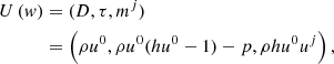
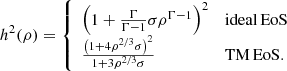
The presented system of five equations in six unknowns is closed by specifying an additional equation of state (EoS), which is usually provided in the form of h = h(Θ) with $\mathrm{\Theta }=\frac{p}{\rho }$. In CRONOS we considered two EoSs: the ideal one, assuming a constant adiabatic index Γ and the Taub-Mathews (TM) EoS (Mathews 1971), which approaches $\mathrm{\Gamma }\to \frac{4}{3}$ in the high-temperature limit and $\mathrm{\Gamma }\to \frac{5}{3}$ in the low-temperature limit. The specific enthalpies are given by

$$\begin{array}{c}\hfill h(\mathrm{\Theta })=\{\begin{array}{cc}1+\frac{\mathrm{\Gamma }}{\mathrm{\Gamma }-1}\mathrm{\Theta }\hfill & \mathrm{ideal}\mathrm{EoS}\hfill \\ \frac{5}{2}\mathrm{\Theta }+\sqrt{\frac{9}{4}{\mathrm{\Theta }}^2+1}\hfill & \mathrm{TM}\mathrm{EoS},\hfill \end{array}\end{array}$$(4)

respectively. For our current purposes, these EoSs are sufficient, although it should be noted that many more are available in the literature (see e.g. Synge 1957; Rezzolla 2013). Due to the modular design of CRONOS, additional EoSs can be easily added in the future by supplying the relevant routines.

2.2. Passive tracer fields

CRONOS provides the option to solve user-defined conservation laws alongside the ones governing the fluid dynamics (see also Kissmann et al. 2018). A prominent use case for this is the treatment of tracers fields ψ, which are passively advected with the fluid flow. Their value remains constant along fluid lines, following the transport equation

$$\begin{array}{c}\hfill ({\partial }_t+\mathit{v}·\mathrm{\nabla })\psi =0.\end{array}$$(5)

A corresponding conservation equation for Ψ = ψD can be found by combining Eqs. (2a) and (5), yielding

$$\begin{array}{c}\hfill {\partial }_t\mathrm{\Psi }+\mathrm{\nabla }·\left(\mathrm{\Psi }\mathit{v}\right)=0.\end{array}$$(6)

This equation was treated in analogy to the mass-conservation equation Eq. (2a) by the fluid solvers.

3. Notation and general structure

3.1. Coordinate systems

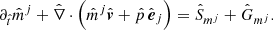
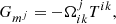
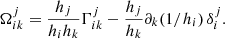
In CRONOS, we employed orthogonal, curvilinear coordinate systems in three dimensions, which are expressed in the generic variables (x¹, x², x³) and the corresponding spatial metric tensor $\gamma =\text{diag}(h_1^2,h_2^2,h_3^2)$ given by the scaling factors h_i. Specifically, we have implemented Cartesian, cylindrical, and spherical coordinates (see also Table A.1). For the latter two, the divergence of the rank-2 stress tensor in the momentum-conservation equation Eq. (2c) yields non-zero geometrical source terms G_m^j. The expression can be expanded component-wise in terms of the standard vector-divergence in the respective coordinate system, yielding

$$\begin{array}{c}\hfill {\partial }_t{m}^j+\mathrm{\nabla }·(m^j\mathit{v}+p{\mathit{e}}_j)=S_{m^j}+G_{m^j},\end{array}$$(7)

where e_j denotes the unit base vector along the jth coordinate direction (see Appendix A).

3.2. Normalisation

For the numerical treatment of the equations, CRONOS uses normalised quantities internally in the form $X=X_0\widehat{X}$, where X is a physical quantity, X₀ a normalisation constant, and $\widehat{X}$ the resulting unit-free, normalised quantity that is treated by the solvers (Kissmann et al. 2018). Our implementation foresees four base quantities that can be normalised independently, which correspond to the length, time, mass, and number density. The latter is not strictly necessary to have a complete system of units. However, it has been proven to be useful in practice since employing a normalisation derived from the length-scale can lead to unwieldy large values for the number density.

The normalisations can be chosen freely by the user, depending on the problem at hand by specifying the normalisation constants for four different quantities, which can also include derived quantities (e.g. energy density, velocity, etc.). If constants for derived quantities are supplied, the normalisations for the non-specified base quantities are obtained automatically via physical relations. If the specified quantities form an inconsistent system of units, the procedure is aborted and the user is notified. In contrast to classical hydrodynamics, velocities are always normalised to the speed of light in the relativistic case, as implicitly imposed by Eqs. (2a)–(2c). The user is hence only allowed to specify the three remaining normalisations to complete the system.

Finally, the normalised equations, corresponding to Eqs. (2a)–(2c), that are solved by CRONOS are

$$\begin{array}{cc}& {\partial }_{\widehat{t}}\widehat{D}+\widehat{\mathrm{\nabla }}·\left(\widehat{D}\widehat{\mathit{v}}\right)={\widehat{S}}_D\hfill \end{array}$$(8a)

$$\begin{array}{cc}& {\partial }_{\widehat{t}}\widehat{\tau }+\widehat{\mathrm{\nabla }}·\left((\widehat{\tau }+\widehat{p})\widehat{\mathit{v}}\right)={\widehat{S}}_{\tau }\hfill \end{array}$$(8b)

$$\begin{array}{cc}& {\partial }_{\widehat{t}}{\widehat{m}}^j+\widehat{\mathrm{\nabla }}·({\widehat{m}}^j\widehat{\mathit{v}}+\widehat{p}{\widehat{\mathit{e}}}_j)={\widehat{S}}_{m^j}+{\widehat{G}}_{m^j}.\hfill \end{array}$$(8c)

For the rest of this work, we exclusively use normalised quantities and omit the hat sign on these for better readability. Once a solution in normalised quantities was obtained, physical quantities could be easily computed in a post-processing step using the corresponding normalisation constants, which are therefore stored together with the data in the output files.

3.3. Grid structure

To solve the set of equations Eqs. (8a)–(8c), CRONOS employs a finite-volume scheme, decomposing the computational volume into a set of disjoint cells (see e.g. LeVeque 2002). While the shapes of the cells are in principle irrelevant for such a scheme, we restricted ourselves to three-dimensional, rectangular grids for practical reasons.

The division into cells is achieved by subdividing each coordinate axis d ∈ {1, 2, 3} spanning the computational domain $(x_{\text{b}}^d,x_e^d)$ into N^d intervals ${\omega }_{i^d}^d$, which are addressed by the index i^d ∈ {0, …, N^d − 1}. The edges of the individual intervals 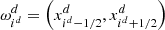${\omega }_{i^d}^d=\left(x_{i^d-1/2}^d,x_{i^d+1/2}^d\right)$ can be freely chosen as long as they are strictly increasing and first and last edges match the beginning and the end of the computational domain, that is $x_{-1/2}^d=x_{\text{b}}^d$ and $x_{N^d-1/2}^d=x_e^d$, respectively. Usually, the edges are chosen to be spaced linearly, however, non-linear options are also implemented (see Kissmann et al. 2018).

The individual cells are then given by 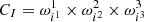$C_I={\omega }_{i^1}^1\times {\omega }_{i^2}^2\times {\omega }_{i^3}^3$ and are correspondingly addressed by the index triplet I = (i¹, i², i³). The centre of a cell $x_I^d≔(x_{i^d-1/2}^d+x_{i^d+1/2}^d)/2$ is defined to be located at the midpoint of each coordinate interval.

A cell C_I borders on a set of neighbouring cells with indices J ∈ N(I). The interfaces to its neighbours Σ_I, J can therefore be used to decompose the cell’s surface as $\partial C_I=\underset{J\in N(I)}{\dot{\bigcup }}{\mathrm{\Sigma }}_{I,J}$. For rectangular grids, the cell interface normals n_I, J are further (anti-)parallel to the d_I, J th coordinate basis vectors, yielding n_I, J ⋅ e_dI, J =0:σ_I, J = ±1.

In contrast to finite difference schemes, where the values of dynamical variables are stored as point values on a grid, in a finite-volume approach, cell-averaged values are stored. The averaged primitive variables $\overline{\mathit{w}}$, which are initially set by the user, are defined by

$$\begin{array}{c}\hfill {\overline{w}}_I≔\frac{1}{\mathrm{\Delta }{V}_I}{{\displaystyle \int }}_{C_I}w\mathrm{d}V\mathrm{with}\mathrm{\Delta }{V}_I≔{{\displaystyle \int }}_{C_I}\mathrm{d}V.\end{array}$$(9)

The corresponding set of averaged conserved variables $\overline{U}$ is defined in analogy.

3.4. Semi-discrete finite-volume scheme

To obtain a numerical scheme to update the cell averages $\overline{\mathit{w}}$ or respectively $\overline{U}$, the set of conservation equations Eq. (1) was integrated over the extent of a cell C_I. Substituting the respective cell averages and applying Gauss’s theorem yields

$$\begin{array}{c}\hfill \frac{\mathrm{d}}{\mathrm{d}t}{\overline{U}}_I={\overline{S}}_I-\frac{1}{\mathrm{\Delta }{V}_I}{\int }_{\partial C_I}\mathit{F}·\mathrm{d}\mathit{A},\end{array}$$(10)

where $\overline{S}$ denotes the cell averaged source term. Splitting the cell’s surface into disjoint interfaces to its neighbours and using the interface-averaged fluxes defined as

$$\begin{array}{c}\hfill {\overline{F}}_{I,J}≔\frac{{\sigma }_{I,J}}{\mathrm{\Delta }{A}_{I,J}}{\displaystyle {\int }_{{\mathrm{\Sigma }}_{I,J}}}{F}^{d_{I,J}}\mathrm{d}A,\mathrm{\Delta }{A}_{I,J}≔{\displaystyle {\int }_{{\mathrm{\Sigma }}_{I,J}}}\mathrm{d}A\end{array}$$(11)

allows Eq. (10) to be rewritten as

$$\begin{array}{c}\hfill \frac{\mathrm{d}}{\mathrm{d}t}{\overline{U}}_I={\overline{\mathcal{L}}}_I≔{\overline{S}}_I-\frac{1}{\mathrm{\Delta }{V}_I}{\displaystyle \sum _{J\in N(I)}\mathrm{\Delta }{A}_{I,J}{\overline{F}}_{I,J}.}\end{array}$$(12)

With this, the initial system of partial differential equations in Eq. (1) has been cast into a system of ordinary differential equations (ODEs) for each grid cell. This is usually referred to as a semi-discrete scheme, since the problem was discretised in space but not in time, having the advantage that the spatial and temporal parts of the problem are conceptually decoupled (see e.g. also Kurganov & Tadmor 2000; LeVeque 2002).

4. Numerical scheme

In CRONOS we followed the general idea presented by Godunov (1959), but used higher-order schemes in both space and time, instead. First, we obtained interface-centred point values of the fluid variables at both sides of a given cell interface using a second-order spatial reconstruction (see Sect. 4.1). The resulting jump in the reconstructed quantities can be viewed as a local, one-dimensional Riemann problem, which was solved by approximate Riemann solvers (see Sect. 4.2) to obtain an estimation for the fluxes ${\overline{F}}_{I,J}$ in Eq. (12). Finally, advancing the solution in time was handled by a second-order Runge-Kutta scheme (see Sect. 4.3).

4.1. Reconstruction

To provide the initial data for the Riemann problems to be solved at the cell interfaces, a spatial reconstruction of the dynamical variables was used. The order of the reconstruction thereby critically determines the spatial accuracy of the overall method. In CRONOS we applied piecewise-linear reconstructions for every coordinate direction independently, using minmod (see van Leer 1979; Harten et al. 1983) and van-Leer (see van Leer 1977) slope limiters. The reconstruction methods employed for special relativistic hydrodynamics are identical to the ones for classical hydrodynamics (see Kissmann et al. 2018).

The reconstruction was applied for primitive variables, yielding the left- (L) and right-handed (R) states ${\mathit{w}}_{I,J}^{\mathrm{L}}$ and ${\mathit{w}}_{I,J}^{\mathrm{R}}$, respectively, at a given cell interface Σ_I, J. Therefrom, the corresponding point values of the conserved variables $U_{I,J}^{\mathrm{L}/\mathrm{R}}$ were computed subsequently. Since the flux function in Eqs. (2a)–(2c) is expressed in terms of primitive variables, this approach has the additional advantage that the more expensive variable conversion from conserved to primitive ones (see Sect. 4.4) can be avoided.

As opposed to Newtonian hydrodynamics, where the fluid speed is generally not bound, it has to remain subluminal at all times for relativistic hydrodynamics. This constraint can be easily violated if three-velocity components are reconstructed independently of each other. In our case, related problems were avoided from the outset since we used and reconstructed spatial four-velocity components instead, which are not subject to such a constraint.

4.2. Approximate Riemann solvers

For a given cell interface Σ_I, J, the reconstructed states at both sides were used to define a local Riemann problem that can be formalised as

$$\begin{array}{c}\hfill w(t_0,\xi )=\{\begin{array}{cc}{w}_{I,J}^{\mathrm{L}}\hfill & \xi <{\xi }_{I,J}\hfill \\ w_{I,J}^{\mathrm{R}}\hfill & \xi >{\xi }_{I,J},\hfill \end{array}\end{array}$$(13)

with ξ = x^d_I, J denoting the coordinate aligned with the interface normal. Assuming the cell-interface to be flat, the conservation Eq. (1) governing the evolution of the Riemann problem reduces to

$$\begin{array}{c}\hfill {\partial }_{t}U+{\partial }_{\xi }f(w)=0,\end{array}$$(14)

where f = e_dI, J ⋅ F = F^d_I, J corresponds to the flux through the interface.

Although relativistic Riemann problems cannot be solved in a closed analytic form, semi-analytic iterative solvers have been developed that can compute their solution to arbitrary precision (see e.g. Marti & Müller 1994; Pons et al. 2000). Employing such solvers, however, is cumbersome and computationally very expensive, which makes them unsuitable for an application in simulation codes.

Instead, approximate Riemann solvers have been developed, making simplifying assumptions on the waves emerging from the initial discontinuity. This significantly reduces the computational cost, while still yielding good approximations for the fluxes at the cell interfaces. In CRONOS we employed the HLL and the HLLC special-relativistic Riemann solvers (Mignone & Bodo 2005). Since every cell interface is treated individually and identically by the solver, we omit the cell indices, for example ${\mathit{w}}_{\mathrm{L}}\equiv {\mathit{w}}_{I,J}^{\mathrm{L}}$, for the remainder of this section for the sake of better readability.

4.2.1. HLL solver

One of the most commonly employed Riemann solvers is the HLL solver first proposed by Harten et al. (1983) for the classical Euler equations. The generalisation to the relativistic case is straightforward and was used in Schneider et al. (1993) for the first time. Here, we briefly summarise the expressions relevant for the implementation in CRONOS.

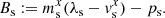
The solver assumes that the Riemann problem produces two shock waves propagating with speeds λ_L and λ_R computed from Eqs. (27a) and (27b). Only one constant intermediate state U^* is considered to be formed between both shocks, while the states ahead of the shocks remain unchanged. The intermediate state can be computed directly from the Rankine-Hugoniot jump conditions at both shocks

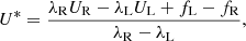$$\begin{array}{c}\hfill U^{\ast }=\frac{{\lambda }_{\mathrm{R}}{U}_{\mathrm{R}}-{\lambda }_{\mathrm{L}}{U}_{\mathrm{L}}+f_{\mathrm{L}}-f_{\mathrm{R}}}{{\lambda }_{\mathrm{R}}-{\lambda }_{\mathrm{L}}},\end{array}$$(15)

using the fluxes of the undisturbed states at either side f_L/R = f(w_L/R). The corresponding fluxes in the intermediate region are then given by

$$\begin{array}{cc}\hfill f^{\ast }& =\frac{{\lambda }_{\mathrm{R}}{f}_{\mathrm{L}}-{\lambda }_{\mathrm{L}}{f}_{\mathrm{R}}+{\lambda }_{\mathrm{L}}{\lambda }_{\mathrm{R}}(U_{\mathrm{R}}-U_{\mathrm{L}})}{{\lambda }_{\mathrm{R}}-{\lambda }_{\mathrm{L}}}·\hfill \end{array}$$(16)

Depending on the signal speeds λ_L/R, the numerical cell-interfaces fluxes are ultimately given by

$$\begin{array}{c}\hfill F^{\mathrm{HLL}}=\{\begin{array}{cc}{f}_{\mathrm{L}}\hfill & \mathrm{for}0<{\lambda }_{\mathrm{L}}\hfill \\ f^{\ast }\hfill & \mathrm{for}{\lambda }_{\mathrm{L}}<0<{\lambda }_{\mathrm{R}}\hfill \\ f_{\mathrm{R}}\hfill & \mathrm{for}{\lambda }_{\mathrm{R}}<0.\hfill \end{array}\end{array}$$(17)

Although the HLL solver is quite simple and computationally inexpensive, it yields good and robust approximations for the cell-interface fluxes. In general, the solver has been found to perform well at shock and rarefaction waves. However, since contact discontinuities were not considered in the simplified wavefan, the HLL solver introduces additional numerical dissipation at such waves.

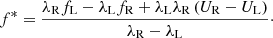
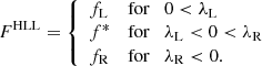
4.2.2. HLLC solver

A natural improvement to the HLL solver is to restore the neglected contact discontinuity. The corresponding approximate Riemann solver, which considers all physical intermediate states, is known as the HLLC solver and was first presented by Toro (1997) for the classical Euler equations and later extended to special relativistic hydrodynamics by Mignone & Bodo (2005). Again, we briefly summarise the quantities relevant for our implementation in CRONOS.

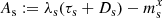
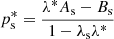
The solver assumes the emerging wavefan to be composed of two shocks together with a contact discontinuity in between, separating two intermediate states $U_{\text{s}}^{*}$ with s ∈ {L, R}, respectively. Using the Rankine-Hugoniot jump conditions for both shock waves and assuming that the intermediate-state fluxes take the following form $f_{\text{s}}^{*}=f(w_{\text{s}}^{*})$, which is not necessarily the case in general (Mignone & Bodo 2005), the speed of the contact discontinuity λ^* is given by

$$\begin{array}{cc}\hfill {\left({\lambda }^{\ast }\right)}^2[{\lambda }_{\mathrm{L}}{A}_{\mathrm{R}}-{\lambda }_{\mathrm{R}}{A}_{\mathrm{L}}]& +[B_{\mathrm{R}}-B_{\mathrm{L}}]\hfill \\ \hfill & -{\lambda }^{\ast }[A_{\mathrm{R}}-A_{\mathrm{L}}+{\lambda }_{\mathrm{L}}{B}_{\mathrm{R}}-{\lambda }_{\mathrm{R}}{B}_{\mathrm{L}}]=0,\hfill \end{array}$$(18)

with

$$\begin{array}{cc}& A_{\mathrm{s}}≔{\lambda }_{\mathrm{s}}({\tau }_{\mathrm{s}}+D_{\mathrm{s}})-m_{\mathrm{s}}^x\hfill \end{array}$$(19)

$$\begin{array}{cc}\hfill & B_{\mathrm{s}}≔m_{\mathrm{s}}^x({\lambda }_{\mathrm{s}}-v_{\mathrm{s}}^x)-p_{\mathrm{s}}.\hfill \end{array}$$(20)

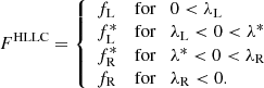
We solved this equation analytically, taking only the root with the minus sign into account since this is the only physically acceptable one (Mignone & Bodo 2005).

After computing the intermediate-state pressure for one side

$$\begin{array}{c}\hfill p_{\mathrm{s}}^{\ast }=\frac{{\lambda }^{\ast }{A}_{\mathrm{s}}-B_{\mathrm{s}}}{1-{\lambda }_{\mathrm{s}}{\lambda }^{\ast }}\end{array}$$(21)

and using the constant pressure over the contact discontinuity 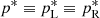$p^{*}\equiv p_{\text{L}}^{*}\equiv p_{\text{R}}^{*}$, the remaining quantities of the intermediate states are given by

$$\begin{array}{cc}& m_{\mathrm{s}}^{x\ast }({\lambda }_{\mathrm{s}}-{\lambda }^{\ast })=m_{\mathrm{s}}^x({\lambda }_{\mathrm{s}}-v_{\mathrm{s}}^x)-p_{\mathrm{s}}+p^{\ast }\hfill \end{array}$$(22)

$$\begin{array}{cc}& {\tau }_{\mathrm{s}}^{\ast }({\lambda }_{\mathrm{s}}-{\lambda }^{\ast })={\tau }_{\mathrm{s}}({\lambda }_{\mathrm{s}}-v_{\mathrm{s}}^x)-v_{\mathrm{s}}^x{p}_{\mathrm{s}}+{\lambda }^{\ast }{p}^{\ast }\hfill \end{array}$$(23)

$$\begin{array}{cc}& {\zeta }_{\mathrm{s}}^{\ast }({\lambda }_{\mathrm{s}}-{\lambda }^{\ast })={\zeta }_{\mathrm{s}}({\lambda }_{\mathrm{s}}-v_{\mathrm{s}}^x).\hfill \end{array}$$(24)

Here, ζ represents any passively advected, conserved quantity such as the mass density D, the momentum densities m^t₁, m^t₂ tangential to the interface, or any generic tracer field Ψ. Finally, the numerical fluxes at the cell interfaces were obtained from

$$\begin{array}{c}\hfill F^{\mathrm{HLLC}}=\{\begin{array}{cc}{f}_{\mathrm{L}}\hfill & \mathrm{for}0<{\lambda }_{\mathrm{L}}\hfill \\ f_{\mathrm{L}}^{\ast }\hfill & \mathrm{for}{\lambda }_{\mathrm{L}}<0<{\lambda }^{\ast }\hfill \\ f_{\mathrm{R}}^{\ast }\hfill & \mathrm{for}{\lambda }^{\ast }<0<{\lambda }_{\mathrm{R}}\hfill \\ f_{\mathrm{R}}\hfill & \mathrm{for}{\lambda }_{\mathrm{R}}<0.\hfill \end{array}\end{array}$$(25)

To avoid a direct evaluation of the flux function $f(w_{\text{s}}^{*})$ for the intermediate states, which would require a variable inversion, the intermediate-state numerical fluxes were computed from the Rankine-Hugoniot conditions instead:

$$\begin{array}{c}\hfill f_{\mathrm{s}}^{\ast }=f_{\mathrm{s}}+{\lambda }_{\mathrm{s}}(U_{\mathrm{s}}^{\ast }-U_{\mathrm{s}}).\end{array}$$(26)

The HLLC solver has been shown to have superior performance compared to the more simple HLL solver. However, it has also been reported to potentially suffer from the carbuncle phenomenon (see e.g. Quirk 1994; Dumbser et al. 2004).

4.2.3. Wave speed estimates

Both the HLL and HLLC Riemann solvers require an estimate for the fastest signal speeds to the left and to the right of the discontinuity λ_L, λ_R, respectively (see also Toro 1997). They can be obtained from the smallest and largest eigenvalues of the system in Eq. (14) and were first computed by Davis (1988) for the relativistic case. Although this is not the only possible estimate (e.g. the Roe average, see Roe 1981), it is commonly used in many codes (see e.g. Mignone et al. 2007; Lamberts et al. 2013). In CRONOS we used

$$\begin{array}{c}\hfill {\lambda }_{\mathrm{L}}=min({\lambda }_{-}(w_{\mathrm{L}}),{\lambda }_{-}\left(w_{\mathrm{R}}\right))\end{array}$$(27a)

$$\begin{array}{c}\hfill {\lambda }_{\mathrm{R}}=max({\lambda }_{+}(w_{\mathrm{L}}),{\lambda }_{+}\left(w_{\mathrm{R}}\right)),\end{array}$$(27b)

where λ_± are the smallest and largest eigenvalues of the system, respectively, which take the form

$$\begin{array}{c}\hfill {\lambda }_{\pm }(w)=\frac{u^0{u}^d\pm \sqrt{u_{\mathrm{s}}^2({u^0}^2-{u^d}^2+u_{\mathrm{s}}^2)}}{{u^0}^2+u_{\mathrm{s}}^2},\end{array}$$(28)

with d = d_I, J corresponding to the direction of the interface normal, 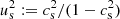$u_{\text{s}}^2≔c_{\text{s}}^2/(1-c_{\text{s}}^2)$, and the sound speed (taken from Mignone & McKinney 2007)

$$\begin{array}{c}\hfill c_{\mathrm{s}}^2(\mathrm{\Theta })=\{\begin{array}{cc}\frac{\mathrm{\Gamma }\mathrm{\Theta }}{h}\hfill & \mathrm{ideal}\mathrm{EoS}\hfill \\ \frac{\mathrm{\Theta }}{3h}+\frac{5h-8\mathrm{\Theta }}{h-\mathrm{\Theta }}\hfill & \mathrm{TM}\mathrm{EoS},\hfill \end{array}\end{array}$$(29)

with h(Θ) being computed from Eq. (4).

4.3. Time integration

In CRONOS, we treated the system of ODEs, arising in the semi-discrete framework in Eq. (12) in time, using a second-order total-variation-diminishing Runge-Kutta scheme, that is Heun’s method (see Shu 1988)

$$\begin{array}{cc}& {\overline{U}}_I^{\ast }={\overline{U}}_I^n+{\overline{\mathcal{L}}}_I\left(w^n\right)\mathrm{\Delta }t\hfill \end{array}$$(30a)

$$\begin{array}{cc}& {\overline{U}}_I^{n+1}=\frac{1}{2}({\overline{U}}_I^n+{\overline{U}}_I^{\ast }+{\overline{\mathcal{L}}}_I\left(w^{\ast }\right)\mathrm{\Delta }t),\hfill \end{array}$$(30b)

where the indices n, n + 1, and indicate values at the current, the next, and an intermediate time-step.

The evaluation of the dimensionally unsplit operator ${\overline{\mathcal{L}}}_I$ for a given cell requires the computation of the numerical fluxes at every cell interface. This involves the solution of Riemann problems, which is the most expensive part of the scheme. Since ${\overline{F}}_{I,J}=-{\overline{F}}_{J,I}$ by construction, we iterated over interfaces in the computational domain instead of over cells to avoid unnecessary double computations. In practice, we further iterated over one-dimensional pencils for each coordinate, which allows for the efficient utilisation of the coordinate-wise nature of the reconstructions. This is followed by another iteration over the whole domain regarding the source term, where we evaluated the respective expressions at the cell centres as

$$\begin{array}{c}\hfill {\overline{S}}_I=S(t,x_I,{\overline{w}}_I).\end{array}$$(31)

The step size for the numerical time integration was constrained by the CFL condition (see Courant et al. 1928) and was obtained from

$$\begin{array}{c}\hfill \mathrm{\Delta }t=C_{\mathrm{CFL}}\underset{I,J}{min}\left(\frac{\mathrm{\Delta }{L}_I^{d_{I,J}}}{{\lambda }_{I,J}^{\max }}\right),\end{array}$$(32)

where C_CFL is the Courant number and ${\lambda }_{I,J}^{\max }$ the largest absolute value of the signal speeds computed at the cell interface Σ_I, J, which was retrieved from the characteristic speeds that have been computed for the Riemann solvers. We allowed the user to set a specific value for C_CFL in each parameter file, individually. For dimensionally unsplit schemes, such as the one described here, the Courant number was chosen to be C_CFL ≤ 1/N_d to maintain stability in any case (see also Lamberts et al. 2013), where N_d is the dimension of the problem. Depending on the problem, however, the condition might be eased; for example, for radially symmetric flows, a Courant number of $C_{\mathrm{CFL}}\le 1/\sqrt{N_d}$ is sufficient. The time step is further adapted if an output checkpoint or the end of the simulation is reached. After obtaining a solution at t^n + 1, user-supplied routines are invoked, for example, to reset the solution in a given region, before the time integration procedure starts again.

In contrast to Newtonian hydrodynamics, where the signal speeds λ^max are not limited in general, they are bound by the speed of light in relativity. In practice, this implies that the step size computed from Eq. (32) does not become smaller than 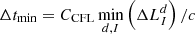$\mathrm{\Delta }{t}_{\text{min}}=C_{\text{CFL}}{\min }_{d,I}\left(\mathrm{\Delta }{L}_I^d\right)/c$, which only depends on the extension of the smallest cell. Such a lower bound has been proven to be useful in practice for the estimation of maximum simulation runtimes.

4.4. Variable inversion

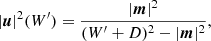
Since the fluxes are given in terms of the primitive fluid variables w = (ρ, p, u^j) but the time integration has to be performed on conserved variables U = (D, τ, m^j) to obtain a shock-capturing scheme, transformations between the two sets are required. While the conversion from primitive quantities to conserved ones is trivial and can be implemented in a straightforward manner, the conversion in the other direction is not and it involves solving non-linear equations for at least one of the quantities. For this, we closely followed the approach presented by Mignone & McKinney (2007), which was initially developed for relativistic MHD, and we adapted it for our purposes (similar to Lamberts et al. 2013). We solved the non-linear equation

$$\begin{array}{c}\hfill f(W^{\prime })≔W^{\prime }-\tau -p(\chi ,\rho )=0,\end{array}$$(33)

where W′=D(hu⁰−1) and χ = ρ(h − 1). The function p(χ, ρ) depends on the chosen EoS and can be found in Table 1 for the different cases implemented in CRONOS. To evaluate f for a given W′, we first computed the corresponding four-speed via

$$\begin{array}{c}\hfill {|\mathit{u}|}^2(W^{\prime })=\frac{{|\mathit{m}|}^2}{{(W^{\prime }+D)}^2-{|\mathit{m}|}^2},\end{array}$$(34)

which was used to obtain (Mignone & McKinney 2007)

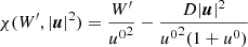$$\begin{array}{c}\hfill {\chi (W^{\prime },|\mathit{u}|}^2)=\frac{W^{\prime }}{{u^0}^2}-\frac{{D|\mathit{u}|}^2}{{u^0}^2(1+u^0)}\end{array}$$(35)

and

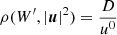$$\begin{array}{c}\hfill {\rho (W^{\prime },|\mathit{u}|}^2)=\frac{D}{u^0}\end{array}$$(36)

employing the identity (u⁰)² = 1 + |u|².

We solved Eq. (33) numerically using an iterative Newton-Raphson scheme until the relative change was below a certain threshold ϵ, which can be set by the user depending on the problem (typically ϵ = 10⁻⁸). It can be shown analytically that the scheme is accurate in the ultra-relativistic limit as long as u⁰ ≲ ϵ^−1/2 and p/(ρu⁰²)≳ϵ (see Mignone & McKinney 2007), which might require an adjustment of ϵ for certain problems.

The derivative  df/ dW′ required by the algorithm is expressed as

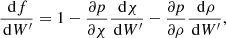$$\begin{array}{c}\hfill \frac{\mathrm{d}f}{\mathrm{d}{W}^{\prime }}=1-\frac{\partial p}{\partial \chi }\frac{\mathrm{d}\chi }{\mathrm{d}{W}^{\prime }}-\frac{\partial p}{\partial \rho }\frac{\mathrm{d}\rho }{\mathrm{d}{W}^{\prime }},\end{array}$$(37)

where the kinematical derivatives are given by

$$\begin{array}{cc}\hfill \frac{\mathrm{d}\chi }{\mathrm{d}{W}^{\prime }}& =\frac{1}{{u^0}^2}+u^0(D+2u^0\chi )\frac{{|\mathit{m}|}^2}{{(W^{\prime }+D)}^3}\hfill \end{array}$$(38)

$$\begin{array}{cc}\hfill \frac{\mathrm{d}\rho }{\mathrm{d}{W}^{\prime }}& =\frac{D{u}^0{|\mathit{m}|}^2}{{(W^{\prime }+D)}^3}·\hfill \end{array}$$(39)

The derivatives involving the pressure ∂_χp and ∂_ρp again depend on the chosen EoS and are also listed in Table 1.

The Newton-Raphson iteration is started using the initial value

$$\begin{array}{c}\hfill W_0^{\prime }=\frac{1}{3}(2E+\sqrt{4E^2-3{|\mathit{m}|}^2})-D.\end{array}$$(40)

This choice guarantees pressure positivity given the conservative state is physically admissible (Mignone & McKinney 2007).

Once a sufficiently precise solution for W′ is found, the primitive variables are given by Eq. (36), p(χ, ρ) supplied by the EoS, and by

$$\begin{array}{c}\hfill \mathit{u}(W^{\prime })=\frac{\mathit{m}}{{(W^{\prime }+D)}^2-{|\mathit{m}|}^2}·\end{array}$$(41)

4.4.1. Admissible conserved states

If a given conserved state is unphysical, the variable inversion fails and produces unphysical primitive states, for example, with negative density or pressure, superluminal speeds, etc., or the inversion does not converge at all. To avoid related problems, we checked the admissibility of a given conserved state U ∈ 𝒢₁ before every inversion, relying on the set of physically admissible states formulated by Wu & Tang (2015):

$$\begin{array}{c}\hfill {\mathcal{G}}_1=\{\mathit{U}|D>0,q(\mathit{U})≔\tau +D-\sqrt{D^2+{|\mathit{m}|}^2}>0\}.\end{array}$$(42)

If the constraint is violated (U ∉ 𝒢₁), the user is informed and the simulation is aborted by default. Alternatively, the user can choose to overwrite the states in the concerned cells with new ones by supplying user-defined routines, for example, setting a lower limit for the pressure and computing other quantities accordingly.

4.4.2. Entropy inversion

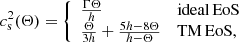
In situations where the thermal energy is negligible compared to the kinetic energy, simple discretisation errors can lead to unphysical states (U ∉ 𝒢₁) for which the variable inversion will fail. To avoid related problems, we offer the user the possibility to solve an additional equation for the conservation of entropy in smooth flows

$$\begin{array}{c}\hfill {\partial }_t\mathrm{\Sigma }+\mathrm{\nabla }·\left(\mathrm{\Sigma }\mathit{v}\right)=0,\end{array}$$(43)

next to the hydrodynamic equations (in analogy to our procedure for classical HD and MHD Kissmann et al. 2018), with Σ = σD and the entropy (Mignone & McKinney 2007)

$$\begin{array}{c}\hfill \sigma =\{\begin{array}{cc}\frac{p}{{\rho }^{\mathrm{\Gamma }}}\hfill & \mathrm{ideal}\mathrm{EoS}\hfill \\ \frac{p}{{\rho }^{5/3}}(h-\mathrm{\Theta })\hfill & \mathrm{TM}\mathrm{EoS}.\hfill \end{array}\end{array}$$(44)

Numerically, the equation was treated in analogy to passive tracer fields (see Sect. 2.2), which guaranteed that we maintained positive values for Σ using the implemented solvers. Although the conservation of energy might be slightly violated by employing Σ instead of τ in the variable inversion, the resulting scheme is much more stable, which can be necessary for certain applications.

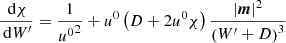
When using Σ, the inversion was performed by numerically solving

$$\begin{array}{c}\hfill g(\rho )=\rho u^0(h(\rho ))-D=0,\end{array}$$(45)

where

$$\begin{array}{c}\hfill u^0(h)=\sqrt{1+\frac{{|\mathit{m}|}^2}{D^2{h}^2}}\end{array}$$(46)

and

$$\begin{array}{c}\hfill h^2(\rho )=\{\begin{array}{cc}{(1+\frac{\mathrm{\Gamma }}{\mathrm{\Gamma }-1}\sigma {\rho }^{\mathrm{\Gamma }-1})}^2\hfill & \mathrm{ideal}\mathrm{EoS}\hfill \\ \frac{{(1+4{\rho }^{2/3}\sigma )}^2}{1+3{\rho }^{2/3}\sigma }\hfill & \mathrm{TM}\mathrm{EoS}.\hfill \end{array}\end{array}$$(47)

Although the derivative of Eq. (45) can be easily found and implemented for a Newton-Raphson scheme to solve the equation, we used a hybrid, bracketing, root-finding method, that is Brent’s method (Brent 1972), instead. For our use cases, we found a comparable performance for both solvers, while the latter one is guaranteed to converge in any case. As an initial bracket for the scheme, we used ρ_max = D and ${\rho }_{\min }=D^2/\sqrt{D^2+{|\mathit{m}|}^2}$. These limits were obtained from ρ = D/u⁰(h) using the asymptotic values of the specific enthalpy 1 < h < ∞ in the ultra-cold and ultra-hot limit, respectively.

Once a sufficiently accurate value for ρ was found, the inversion was completed by computing the fluid velocity from u = m/Dh(ρ) and the pressure according to

$$\begin{array}{c}\hfill p=\{\begin{array}{cc}\sigma {\rho }^{\mathrm{\Gamma }}\hfill & \mathrm{ideal}\mathrm{EoS}\hfill \\ \frac{1}{2}\rho (h(\rho )-\sqrt{h^2(\rho )-4\sigma {\rho }^{2/3}})\hfill & \mathrm{TM}\mathrm{EoS}.\hfill \end{array}\end{array}$$(48)

The conservation of entropy, however, only applies for smooth, non-compressive flows. To identify those cells for which this is the case and the variable inversion can be feasibly performed using Eq. (45), we flagged cells according to the following criteria (similar to Balsara & Spicer 1999; Mignone et al. 2020):

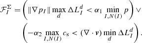$$\begin{array}{cc}\hfill {\mathcal{F}}_I^{\mathrm{\Sigma }}=& (\parallel \mathrm{\nabla }{p}_I\parallel \underset{d}{max}\mathrm{\Delta }{L}_I^d<{\alpha }_1\underset{I,N(I)}{min}p)\vee \hfill \\ \hfill & (-{\alpha }_2\underset{I,N(I)}{max}{c}_{\mathrm{s}}<(\mathrm{\nabla }·\mathit{v})\underset{d}{min}\mathrm{\Delta }{L}_I^d).\hfill \end{array}$$(49)

The occurring gradient and divergence were approximated using central, finite differences and c_s denotes the local sound speed computed according to Eq. (29). We typically used values of α₁ = 0.05 and α₂ = 0. Further, if a given cell I did not qualify for the entropy inversion (${\mathcal{F}}_I^{\mathrm{\Sigma }}=0$), we also disabled the flag for its direct neighbours for safety (${\mathcal{F}}_J^{\mathrm{\Sigma }}=0$ for J ∈ N(I)).

Wherever ${\mathcal{F}}_I^{\mathrm{\Sigma }}=1$, we performed the variable inversion using Eq. (45). Otherwise, Eq. (33) was used and the corresponding value of σ was recomputed from the resulting state. The described procedure can be enabled or disabled by a compile-time switch set by the user.

5. Validation

In the following sections, we present the results from a variety of numerical tests to verify our implementations within the CRONOS code.

5.1. 1D Riemann problems

One-dimensional Riemann problems are particularly useful numerical tests for hydrodynamic codes since they can be solved by semi-analytical methods to arbitrary precision (Marti & Müller 1994). The Riemann problems for the following tests are posed in the general form

$$\begin{array}{c}\hfill (\rho ,v^x,p)=\{\begin{array}{cc}{w}_{\mathrm{L}}\hfill & \mathrm{for}x<0.5\hfill \\ w_{\mathrm{R}}\hfill & \mathrm{for}x>0.5.\hfill \end{array}\end{array}$$(50)

For comparison, we considered the same set of Riemann problems as in Mignone & Bodo (2005), summarised in Table 2 with zero fluid velocity tangential to the discontinuity and an ideal EoS with $\mathrm{\Gamma }=\frac{5}{3}$. All numerical tests were performed using extrapolating boundary conditions.

In Fig. 1, we present the numerical evolution of the considered Riemann problems together with their exact solutions¹. In P1 and P2, two shock waves and two rarefaction waves are formed, respectively, which are in good agreement with the exact solutions. The tests P3 and P4 are characterised by large differences in pressure between the initial states and they evolve into a leftward-moving rarefaction and a rightward-moving shock wave, forming dense shells of material. These shells are also known as relativistic blast waves and pose notoriously difficult problems for numerical schemes. For P4, the numerical solution yields a shock position and a compression ratio that slightly differ from their exact locations and values. This is caused by an insufficient resolution of the blast wave in combination with the spatial reconstruction effectively reducing to first order in the vicinity of shocks. Overall, the numerical solutions obtained using CRONOS are in good agreement with the exact, semi-analytic solutions, which validates the implemented solvers.

Fig. 1. Numerical results for one-dimensional Riemann problems at time t = 0.4. The density (blue crosses) and pressure (orange plus signs) are shown. The underlying solid black line corresponds to the exact solution. The numerical solutions have been obtained using 400 gridpoints, the minmod slope limiter, the HLLC solver, and CFL = 0.4. To improve visibility, we show only every fourth point of the numerical results and scaled the different quantities as annotated. The parametrisations of the Riemann problems for the numerical test can be found in Table 2.

5.2. 1D Riemann problems with non-zero tangential velocity

While velocities tangential to the initial discontinuity v^t do not affect the evolution of Riemann problems in classical hydrodynamics, they do have a severe impact on the emerging wavefan in relativistic hydrodynamics because of the non-linear coupling introduced by the Lorentz factor. We demonstrated that these effects are also correctly handled by our implementations by solving the Riemann problem

$$\begin{array}{c}\hfill (\rho ,v^x,v^t,p)=\{\begin{array}{cc}(1,0.5,0,1)\hfill & \mathrm{for}x<0.5\hfill \\ (0.125,0,v_{\mathrm{R}}^t,0.1)\hfill & \mathrm{for}x>0.5\hfill \end{array}\end{array}$$(51)

for different values of the right-sided, tangential velocity $v_{\text{R}}^t$ in analogy to the ones in Sect. 5.1. Exact semi-analytic solutions with non-zero tangential velocities¹ are again available in the literature (see Pons et al. 2000; Rezzolla et al. 2003), which were used to produce the reference solutions shown in Fig. 2.

Fig. 2. Same as in Fig. 1, but for Riemann problems involving non-zero tangential velocities in the right state with $v_{\text{R}}^t=0.7$ (top) and $v_{\text{R}}^t=0.9$ (bottom) as parameterised in Eq. (51). The solutions for the tangential velocity (green crosses) and the pressure (orange plus signs) are shown.

We investigated two scenarios with $v_{\text{R}}^t=0.7$ and $v_{\text{R}}^t=0.9$ and show the numerical solutions in Fig. 2. The numerical results agree well with the exact solutions and show the transition from a rarefaction-shock to a shock-shock pattern expected at $v_{\text{R}}^t~0.85$ (Rezzolla et al. 2003). The numerical L₁ errors are $L_1^{\rho }=6.20\times {10}^{-3};9.76\times {10}^{-3}$ for the density and $L_1^p=6.61\times {10}^{-3};9.04\times {10}^{-3}$ for the pressure, corresponding to $v_{\text{R}}^t=0.7;0.9$, respectively.

5.3. 2D Riemann problem

After the successful tests in one dimension, we now move to tests in higher dimensions. First, we consider a two-dimensional Riemann problem, which is posed by the interaction of four different initial states; one in each quadrant of the two-dimensional plane. For the sake of comparison, we solved the same problem as investigated by Del Zanna & Bucciantini (2002) that is parameterised as

$$\begin{array}{c}\hfill (\rho ,v^x,v^y,p)=\{\begin{array}{cc}(0.1,0,0,0.01)\hfill & \mathrm{for}x>0,y>0\hfill \\ (0.1,0.99,0,1)\hfill & \mathrm{for}x<0,y>0\hfill \\ (0.5,0,0,1)\hfill & \mathrm{for}x<0,y<0\hfill \\ (0.1,0,0.99,1)\hfill & \mathrm{for}x>0,y<0.\hfill \end{array}\end{array}$$(52)

Again, we used extrapolating boundary conditions, the minmod slope limiter, and an ideal EoS with $\mathrm{\Gamma }=\frac{5}{3}$.

In Fig. 3, we present the numerical results using the HLL and HLLC solver, respectively. The initial discontinuities separating the two top states and the two right states evolve into curved shock waves that enclose a drop-shaped region in the top-right quadrant. The lower-left region remains confined by two contact discontinuities and forms a jet-like structure. While the contact discontinuities remain sharp and steady using the HLLC solver, they degenerate into spurious waves using the HLL solver because of the increased numerical dissipation of the latter, demonstrating the better performance of the HLLC solver. Our numerical results agree well with the ones in the literature (e.g. Del Zanna & Bucciantini 2002; Mignone & Bodo 2005). Having verified the implementation on Cartesian grids, we moved to curvilinear coordinates in the subsequent test.

Fig. 3. Logarithmically equidistant contours of the rest-mass density for numerical solutions of the two-dimensional Riemann problem given in Eq. (52) at time t = 0.8. The results using the HLL solver (top) and HLLC solver (bottom) are shown, respectively. The solutions were obtained on a grid with 4002 cells using a CFL number of 0.4.

5.4. Axisymmetric relativistic jet

In this numerical test, we demonstrate the implementation of geometric source terms arising in non-Cartesian coordinate systems (see Sect. 3.1). For this, we simulated the evolution of an axisymmetric relativistic jet in 2D cylindrical geometry. The jet was set up by initialising the computational volume with an ambient, background medium (respective quantities are denoted with an index m) and injecting the supersonic beam material (denoted with an index b) by imposing constant boundary conditions at z = 0 for radii r < 1. At the symmetry axis of the jet r = 0, we imposed reflecting boundary conditions and outflowing boundary conditions everywhere else. The computational domain covers the region 0 ≤ r ≤ 12 and 0 ≤ z ≤ 35. For the sake of comparison, we adopted the same set of parameters as Del Zanna & Bucciantini (2002), which are given by the beam density ρ_b = 0.1, the beam speed $v_{\text{b}}^z=0.99$, the ambient medium density ρ_m = 10, matched pressures p_b = p_m = 10⁻², and an ideal EoS with $\mathrm{\Gamma }=\frac{5}{3}$. The ambient medium is at rest, v_m = 0, and the beam has no radial velocity, $v_{\text{b}}^r=0$.

The results at time t = 80 are shown in Fig. 4 and exhibit typical features of relativistic jets, such as the bow-like shock of the ambient medium, a hull of shocked material, a central relativistic stream, and turbulence excited by the Kelvin-Helmholtz instability due to the high velocity shear. Simulations using the HLLC solver show more small-scale fluctuations than those using the HLL solver because of the latter’s higher numerical dissipation. This again demonstrates the superior performance of the HLLC solver. The results are in good qualitative agreement with the numerical solutions obtained by Del Zanna & Bucciantini (2002) and Mignone & Bodo (2005). The slight extension of the head using the HLLC solver is potentially caused by the carbuncle problem, which usually manifests itself as an extended nose on the jet axis (Quirk 1994) and has also been seen in other implementations of this test (e.g. see Lamberts et al. 2013).

Fig. 4. Rest-mass density for the relativistic jet given in Sect. 5.4 at time t = 80. The results using the HLL solver (left half) and HLLC solver (right half) are shown, respectively. The numerical solutions were obtained on a grid with 512 × 1536 cells in cylindrical axisymmetry using a CFL number of 0.4.

Here, we exclusively considered a single ideal EoS. The evolution of relativistic jets, however, is heavily affected by the particular choice of the EoS, which is exploited in the next tests.

5.5. Equation of state

Here we verify the different EoSs implemented in CRONOS (see also Sect. 2). For this, we again simulated the propagation of relativistic jets in analogy to the setup in Sect. 5.4. For a given equation of state, the properties of a jet are determined by three parameters: the density ratio η = ρ_b/ρ_m, the beam’s Lorentz factor $u_{\text{b}}^0$, and its Mach number M_b = v_b/c_s. Following the tests performed in Mignone et al. (2007), we adopted the same jet parameters $\eta ={10}^{-3},u_{\text{b}}^0=10,M_{\text{b}}=1.77$ and investigated the jet evolution under three different EoSs: two ideal ones with $\mathrm{\Gamma }=\frac{5}{3}$ and $\mathrm{\Gamma }=\frac{4}{3}$ and the TM EoS. We further chose the pressures p_b = p_m = 10⁻² resulting in the ambient medium densities ρ_m listed in Table 3, which were used together with ρ_b = η ρ_m and v_b = 0.995 to specify the setup for the simulation.

In Fig. 5 we show the resulting densities for the simulated jets at t = 60. Owing to the different EoSs, the head of the jets propagate at different speeds along the z-axis, which is visible from the different jet extents in the simulation.

Fig. 5. Rest-mass densities for the jets simulated with different equations of state (as annotated) at t = 60. The computations were performed on a grid with 512 × 1536 cells in cylindrical symmetry using the HLLC solver and CFL = 0.4. The jets were set up using the parameters given in the text and Table 3.

In one dimension, the propagation of relativistic jets was investigated by Martí et al. (1997) who derived the following analytical expression for the speed of the head of a jet:

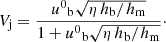$$\begin{array}{c}\hfill V_{\mathrm{j}}=\frac{{u^0}_{\mathrm{b}}\sqrt{\eta h_{\mathrm{b}}/h_{\mathrm{m}}}}{1+{u^0}_{\mathrm{b}}\sqrt{\eta h_{\mathrm{b}}/h_{\mathrm{m}}}}·\end{array}$$(53)

The values corresponding to our setups can again be found in Table 3, which serve as a test for our implementations. In Fig. 6 we show the locations of the jet heads in our numerical simulations, which are in good agreement with the analytical estimates from Eq. (53). As expected from similar simulations performed by Mignone et al. (2007), the simulated jets become slower and start to deviate from the linear propagation in one dimension for later times, which follows from the two-dimensional nature of the numerical tests.

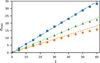Fig. 6. Position of the head of the jet over time for different equations of state: $\mathrm{\Gamma }=\frac{5}{3}$ (orange, circles, dashed), $\mathrm{\Gamma }=\frac{4}{3}$ (blue, squares, dash-dotted), TM-EoS (green, triangles, dotted). Markers correspond to numerical results and lines to one-dimensional estimates given by Eq. (53). The simulated jets correspond to the ones depicted in Fig. 5.

5.6. Spatial order

Finally, we verified the order of our scheme using similar tests as those performed for classical hydrodynamics with CRONOS (see Ryu & Goodman 1994; Kissmann et al. 2018). These tests investigate the decay of two-dimensional standing sound waves by the numerical dissipation of the scheme.

In analogy to classical hydrodynamics, also in special relativity, acoustic waves can be excited by adding velocity perturbations to a constant background state, owing to the similar structure of the eigenvectors of the linearised equations (see Rezzolla 2013). We initialised sinusoidal sound waves using

$$\begin{array}{c}\hfill \delta u^x=\delta u^y={\delta }_{\mathrm{amp}}sin(k_{x}x+k_{y}y),\end{array}$$(54)

with the perturbation amplitude δ_amp = 10⁻⁵, the wavenumbers $k_x=k_{\mathit{y}}=\frac{2\pi }{L}$, and the side length of the computational domain L = 1. This produces two acoustic waves that propagate with velocities λ_±(w₀) into opposite directions, which can be computed from Eq. (28) for a given constant background state w₀. For the purpose of this test, we chose the background density ρ₀ = 1 and the four-velocity $u_0^x=u_0^y=0,u_0^z=\text{const}.$ to ensure that both waves travel at the same speed, yielding

$$\begin{array}{c}\hfill {\lambda }_{\pm }=\pm c_{\mathrm{s}}\sqrt{\frac{1-{(v_0^z)}^2}{1-{(v_0^z)}^2{c}_{\mathrm{s}}^2}},\end{array}$$(55)

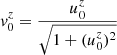where ${\mathit{v}}_0^z=\frac{u_0^z}{\sqrt{1+{(u_0^z)}^2}}$ is the three-speed in z-direction and c_s the sound speed of the background medium, respectively.

In a periodic domain, this produces a standing wave that oscillates with frequency $f=\frac{\sqrt{2}}{L{\lambda }_{+}}$. To introduce relativistic effects, we set the background speed to a relativistic value of $u_0^z=\frac{2}{\sqrt{3}}$. Choosing $c_{\mathrm{s}}=\frac{1}{2}$, which implies $p_0=\frac{3}{4{\rho }_0}$ for an ideal EoS with $\mathrm{\Gamma }=\frac{4}{3}$, therefore leads to one oscillation in two units of time. By simulating until t = 20, we thus captured ten full oscillations.

From the simulations, we retrieved the spatial root-mean-squared average of the velocity perturbation that oscillates with the double frequency. Due to the presence of numerical viscosity, its amplitude decreases exponentially ∝exp(−Γ_decay t). The decay rate Γ_decay was determined from the simulation results as a function of spatial resolution and is shown in Fig. 7. The second-order nature of our scheme is obvious from Γ_decay ∝ N⁻². As expected, the HLLC solver introduces less numerical viscosity as compared to the HLL solver. In both cases we used the minmod slope limiter and CFL = 0.4.

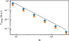Fig. 7. Damping rate Γdecay for the decaying, sound-waves test (see Sect. 5.6) as a function of the number of grid cells N using the HLL (blue circles) and the HLLC solver (orange triangles), respectively. The black dotted line indicates a N−2 dependence to guide the eye.

6. Parallel performance

The relativistic extension of CRONOS has been successfully employed in various computational environments using up to ∼10⁴ computing cores. The code was parallelised using a halo-communication approach that was realised employing the Message Passing Interface (MPI) library.

To test the parallel efficiency of our code, we performed a weak-scaling test on the Joliot-Curie Rome HPC environment with AMD Rome (Epyc) 7H12 2.6GHz bi-processor compute nodes. As a test setup, we considered the colliding winds of two spherically symmetric, static sources similar to the simulation of gamma-ray binaries in Huber et al. (2021a). Initially, the system was divided into two regions, each filled by one of the winds, using an approximate curve for the contact discontinuity in the system. The simulation was run sufficiently long to obtain a representative average of the time step duration. While the domain size was increased with each test, the workload handled by each computation core was kept constant at 64³ cells. The results are shown in Fig. 8. As expected, the parallel efficiency drops with an increasing number of cores, but remains above 93% for more than 1.6 × 10⁴ cores.

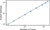Fig. 8. Scaled speedup of simulations performed using CRONOS as a function of the number of computation cores in a weak-scaling test. The dotted line indicates perfect scaling.

7. Summary

We have presented and verified an extension to the CRONOS code treating special relativistic hydrodynamics for astrophysical applications. The code is based on a semi-discrete finite-volume framework, ensuring the conservation of relevant quantities to efficiently capture shocks. CRONOS employs a second-order spatial reconstruction combined with a second-order Runge-Kutta time-integrator. The extension was developed with a focus on robustness, providing the user with additional interfaces to prevent, detect, and possibly counteract failures.

Our implementation was verified against a set of standard problems, for which either an analytical solution or established numerical solutions from the literature are available. Parallel scaling for up to ∼10⁴ cores has been demonstrated.

As the rest of the CRONOS framework, this extension was also developed with modularity in mind, making it easy to consider additional physics supplied by the user. This was, for example, used to simulate an additional transport of energetic particles governed by a Fokker-Planck type equation alongside the fluid dynamics (as demonstrated in Huber et al. 2021a,b).

Acknowledgments

We thankfully acknowledge the access to the research infrastructure of the Institute for Astro- and Particle Physics at the University of Innsbruck (Server Quanton AS-220tt-trt8n16-g11 x8), the LEO HPC infrastructure of the University of Innsbruck and PRACE resources, that were used throughout the development of the code. We acknowledge PRACE for granting us access to Joliot-Curie at GENCI@CEA, France. D.H. acknowledges financial support by the University of Innsbruck through the stipend grant 2020/2/MIP-15 titled “Doktoratsstipendium aus der Nachwuchsförderung”. This research made use of Cronos (Kissmann et al. 2018); GNU Scientific Library (GSL) (Galassi et al. 2018); matplotlib, a Python library for publication quality graphics (Hunter 2007); Scipy (Virtanen et al. 2020); and NumPy (Harris et al. 2020). We thank the anonymous referee for the thoughtful comments and suggestions that allowed us to improve our manuscript.

References

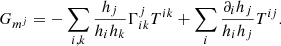
Appendix A: Geometrical source terms

The geometrical source terms G_m^j arising in Eq. (7) can be obtained using the anholonomic connection symbol ${\mathrm{\Omega }}_{\mathit{ik}}^j$ in the given coordinate system as

$$\begin{array}{c}\hfill G_{m^j}=-{\mathrm{\Omega }}_{\mathit{ik}}^j{T}^{\mathit{ik}},\end{array}$$(A.1)

where T^ij = mⁱv^j + p δ^ij denotes the stress-tensor components. The connection symbol corresponds to the anholonomic components of the Christoffel symbol of second kind ${\mathrm{\Gamma }}_{\mathit{ik}}^j$ (also known as natural connection) in physical units and can be computed by (see Altman & de Oliveira 2011)

$$\begin{array}{c}\hfill {\mathrm{\Omega }}_{\mathit{ik}}^j=\frac{h_j}{h_i{h}_k}{\mathrm{\Gamma }}_{\mathit{ik}}^j-\frac{h_j}{h_k}{\partial }_k(1/h_i){\delta }_i^j.\end{array}$$(A.2)

This yields the geometrical source terms

$$\begin{array}{c}\hfill G_{m^j}=-{\displaystyle \sum _{i,k}\frac{h_j}{h_i{h}_k}{\mathrm{\Gamma }}_{\mathit{ik}}^j{T}^{\mathit{ik}}+\sum _i\frac{{\partial }_i{h}_j}{h_i{h}_j}{T}^{\mathit{ij}}.}\end{array}$$(A.3)

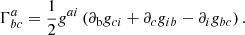
The Christoffel symbol can be readily obtained from the metric tensor g_ij = h_ih_jδ_ij and its derivatives via

$$\begin{array}{c}\hfill {\mathrm{\Gamma }}_{\mathit{bc}}^a=\frac{1}{2}{g}^{\mathit{ai}}({\partial }_{\mathrm{b}}{g}_{\mathit{ci}}+{\partial }_c{g}_{\mathit{ib}}-{\partial }_i{g}_{\mathit{bc}}).\end{array}$$(A.4)

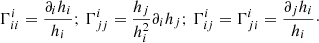
For orthogonal coordinates (Stone & Norman 1992), the only non-zero entries are given by

$$\begin{array}{c}\hfill {\mathrm{\Gamma }}_{\mathit{ii}}^i=\frac{{\partial }_i{h}_i}{h_i};{\mathrm{\Gamma }}_{\mathit{jj}}^i=\frac{h_j}{h_i^2}{\partial }_i{h}_j;{\mathrm{\Gamma }}_{\mathit{ij}}^i={\mathrm{\Gamma }}_{\mathit{ji}}^i=\frac{{\partial }_j{h}_i}{h_i}·\end{array}$$(A.5)

The resulting source terms for the implemented coordinate systems are summarised in Table A.1. We note that the source terms arising in special relativistic hydrodynamics are formally identical to the ones in Newtonian hydrodynamics. This is intuitive since both sets of equations are also formally identical except for different definitions of the conserved variables.

A similar procedure can also be used to derive the source terms for co-rotating coordinate systems in special relativistic hydrodynamics. This has been done in Huber et al. (2021a) in the context of simulation of gamma-ray binaries and is also available in CRONOS.

All Tables

All Figures

Fig. 1. Numerical results for one-dimensional Riemann problems at time t = 0.4. The density (blue crosses) and pressure (orange plus signs) are shown. The underlying solid black line corresponds to the exact solution. The numerical solutions have been obtained using 400 gridpoints, the minmod slope limiter, the HLLC solver, and CFL = 0.4. To improve visibility, we show only every fourth point of the numerical results and scaled the different quantities as annotated. The parametrisations of the Riemann problems for the numerical test can be found in Table 2.

In the text

	Fig. 2. Same as in Fig. 1, but for Riemann problems involving non-zero tangential velocities in the right state with $v_{\text{R}}^t=0.7$ (top) and $v_{\text{R}}^t=0.9$ (bottom) as parameterised in Eq. (51). The solutions for the tangential velocity (green crosses) and the pressure (orange plus signs) are shown.
In the text

	Fig. 3. Logarithmically equidistant contours of the rest-mass density for numerical solutions of the two-dimensional Riemann problem given in Eq. (52) at time t = 0.8. The results using the HLL solver (top) and HLLC solver (bottom) are shown, respectively. The solutions were obtained on a grid with 4002 cells using a CFL number of 0.4.
In the text

	Fig. 4. Rest-mass density for the relativistic jet given in Sect. 5.4 at time t = 80. The results using the HLL solver (left half) and HLLC solver (right half) are shown, respectively. The numerical solutions were obtained on a grid with 512 × 1536 cells in cylindrical axisymmetry using a CFL number of 0.4.
In the text

	Fig. 5. Rest-mass densities for the jets simulated with different equations of state (as annotated) at t = 60. The computations were performed on a grid with 512 × 1536 cells in cylindrical symmetry using the HLLC solver and CFL = 0.4. The jets were set up using the parameters given in the text and Table 3.
In the text

	Fig. 6. Position of the head of the jet over time for different equations of state: $\mathrm{\Gamma }=\frac{5}{3}$ (orange, circles, dashed), $\mathrm{\Gamma }=\frac{4}{3}$ (blue, squares, dash-dotted), TM-EoS (green, triangles, dotted). Markers correspond to numerical results and lines to one-dimensional estimates given by Eq. (53). The simulated jets correspond to the ones depicted in Fig. 5.
In the text

	Fig. 7. Damping rate Γdecay for the decaying, sound-waves test (see Sect. 5.6) as a function of the number of grid cells N using the HLL (blue circles) and the HLLC solver (orange triangles), respectively. The black dotted line indicates a N−2 dependence to guide the eye.
In the text

	Fig. 8. Scaled speedup of simulations performed using CRONOS as a function of the number of computation cores in a weak-scaling test. The dotted line indicates perfect scaling.
In the text

References

- Aloy, M. A., Ibáñez, J. M., Martí, J. M., & Müller, E. 1999, ApJS, 122, 151 [NASA ADS] [CrossRef] [Google Scholar]
- Altman, W., & de Oliveira, A. M. 2011, Mech. Adv. Mater. Struct., 18, 454 [Google Scholar]
- Baiotti, L., Hawke, I., Montero, P. J., et al. 2005, Phys. Rev. D, 71, 024035 [NASA ADS] [CrossRef] [Google Scholar]
- Balsara, D. S., & Spicer, D. 1999, J. Comput. Phys., 148, 133 [NASA ADS] [CrossRef] [Google Scholar]
- Banyuls, F., Font, J. A., Ibáñez, J. M., Martí, J. M., & Miralles, J. A. 1997, ApJ, 476, 221 [NASA ADS] [CrossRef] [Google Scholar]
- Barkov, M. V., Lyutikov, M., Klingler, N., & Bordas, P. 2019, MNRAS, 485, 2041 [NASA ADS] [CrossRef] [Google Scholar]
- Brent, R. P. 1972, Algorithms for Minimization without Derivatives (Englewood Cliffs: Prentice-Hall) [Google Scholar]
- Busza, W., Rajagopal, K., & van der Schee, W. 2018, Annu. Rev. Nucl. Part. Sci., 68, 339 [NASA ADS] [CrossRef] [Google Scholar]
- Courant, R., Friedrichs, K., & Lewy, H. 1928, Math. Ann., 100, 32 [NASA ADS] [CrossRef] [MathSciNet] [Google Scholar]
- Davis, S. F. 1988, SIAM J. Sci. Stat. Comput., 9, 445 [CrossRef] [Google Scholar]
- Del Zanna, L., & Bucciantini, N. 2002, A&A, 390, 1177 [NASA ADS] [CrossRef] [EDP Sciences] [Google Scholar]
- Dumbser, M., Moschetta, J.-M., & Gressier, J. 2004, J. Comput. Phys., 197, 647 [NASA ADS] [CrossRef] [Google Scholar]
- Galassi, M., Davies, J., Theiler, J., et al. 2018, GNU Scientific Library Reference Manual, https://www.gnu.org/software/gsl/ [Google Scholar]
- Godunov, S. K. 1959, Mat. Sb., 3, 271 [Google Scholar]
- Harris, C. R., Millman, K. J., van der Walt, S. J., et al. 2020, Nature, 585, 357 [CrossRef] [PubMed] [Google Scholar]
- Harten, A., Lax, P. D., & van Leer, B. 1983, SIAM Rev., 25, 35 [Google Scholar]
- Huber, D., Kissmann, R., Reimer, A., & Reimer, O. 2021a, A&A, 646, A91 [NASA ADS] [CrossRef] [EDP Sciences] [Google Scholar]
- Huber, D., Kissmann, R., & Reimer, O. 2021b, A&A, 649, A71 [EDP Sciences] [Google Scholar]
- Hunter, J. D. 2007, Comput. Sci. Eng., 9, 90 [NASA ADS] [CrossRef] [Google Scholar]
- Kissmann, R., Kleimann, J., Krebl, B., & Wiengarten, T. 2018, ApJS, 236, 53 [Google Scholar]
- Komissarov, S., & Porth, O. 2021, New Astron. Rev., 92, 101610 [Google Scholar]
- Kurganov, A., & Tadmor, E. 2000, J. Comput. Phys., 160, 241 [Google Scholar]
- Lamberts, A., Fromang, S., Dubus, G., & Teyssier, R. 2013, A&A, 560, A79 [NASA ADS] [CrossRef] [EDP Sciences] [Google Scholar]
- Landau, L. D., & Lifshitz, E. M. 1959, Fluid Mechanics (Oxford: Pergamon Press) [Google Scholar]
- LeVeque, R. J. 2002, Finite Volume Methods for Hyperbolic Problems, Cambridge Texts in Applied Mathematics (Cambridge: Cambridge University Press) [Google Scholar]
- Marti, J. M., & Müller, E. 1994, J. Fluid Mech., 258, 317 [NASA ADS] [CrossRef] [Google Scholar]
- Martí, J. M., Müller, E., Font, J. A., Ibáñez, J. M. Z., & Marquina, A. 1997, ApJ, 479, 151 [NASA ADS] [CrossRef] [Google Scholar]
- Martí, J. M., & Müller, E. 2003, Liv. Rev. Relativ., 6, 7 [Google Scholar]
- Martí, J. M., & Müller, E. 2015, Liv. Rev. Comput. Astrophys., 1, 3 [NASA ADS] [CrossRef] [Google Scholar]
- Mathews, W. G. 1971, ApJ, 165, 147 [NASA ADS] [CrossRef] [Google Scholar]
- Meliani, Z., Keppens, R., Casse, F., & Giannios, D. 2007, MNRAS, 376, 1189 [NASA ADS] [CrossRef] [Google Scholar]
- Mignone, A., & Bodo, G. 2005, MNRAS, 364, 126 [Google Scholar]
- Mignone, A., & McKinney, J. C. 2007, MNRAS, 378, 1118 [Google Scholar]
- Mignone, A., Bodo, G., Massaglia, S., et al. 2007, ApJS, 170, 228 [Google Scholar]
- Mignone, A., Zanni, C., Tzeferacos, P., et al. 2012, ApJS, 198, 7 [Google Scholar]
- Mignone, A., Zanni, C., Vaidya, B., et al. 2020, Pluto User’s Guide v4.4, http://plutocode.ph.unito.it [Google Scholar]
- Mościbrodzka, M., Falcke, H., Shiokawa, H., & Gammie, C. F. 2014, A&A, 570, A7 [NASA ADS] [CrossRef] [EDP Sciences] [Google Scholar]
- Mościbrodzka, M., Falcke, H., & Shiokawa, H. 2016, A&A, 586, A38 [NASA ADS] [CrossRef] [EDP Sciences] [Google Scholar]
- Olmi, B., & Bucciantini, N. 2019, MNRAS, 484, 5755 [NASA ADS] [CrossRef] [Google Scholar]
- Pons, J. A., Ma Martí, J., & Müller, E. 2000, J. Fluid Mech., 422, 125 [NASA ADS] [CrossRef] [Google Scholar]
- Quirk, J. J. 1994, Int. J. Numer. Meth. Fluids, 18, 555 [NASA ADS] [CrossRef] [Google Scholar]
- Reitberger, K., Kissmann, R., Reimer, A., & Reimer, O. 2017, ApJ, 847, 40 [Google Scholar]
- Rezzolla, L. 2013, Relativistic Hydrodynamics (Oxford: Oxford University Press) [CrossRef] [Google Scholar]
- Rezzolla, L., Zanotti, O., & Pons, J. A. 2003, J. Fluid Mech., 479, 199 [NASA ADS] [CrossRef] [Google Scholar]
- Roe, P. L. 1981, in The Use of the Riemann Problem in Finite Difference Schemes, eds. W. C. Reynolds, & R. W. MacCormack, 141, 354 [NASA ADS] [Google Scholar]
- Ryu, D., & Goodman, J. 1994, ApJ, 422, 269 [NASA ADS] [CrossRef] [Google Scholar]
- Scherer, K., Baalmann, L. R., Fichtner, H., et al. 2020, MNRAS, 493, 4172 [Google Scholar]
- Schneider, V., Katscher, U., Rischke, D. H., et al. 1993, J. Comput. Phys., 105, 92 [NASA ADS] [CrossRef] [MathSciNet] [Google Scholar]
- Shu, C.-W. 1988, SIAM J. Sci. Stat. Comput., 9, 1073 [Google Scholar]
- Siegel, D. M., & Metzger, B. D. 2018, ApJ, 858, 52 [CrossRef] [Google Scholar]
- Stone, J. M., & Norman, M. L. 1992, ApJS, 80, 753 [Google Scholar]
- Stone, J. M., Gardiner, T. A., Teuben, P., Hawley, J. F., & Simon, J. B. 2008, ApJS, 178, 137 [NASA ADS] [CrossRef] [Google Scholar]
- Synge, J. L. 1957, The Relativistic Gas (Amsterdam: North-Holland Pub) [Google Scholar]
- Teyssier, R. 2002, A&A, 385, 337 [NASA ADS] [CrossRef] [EDP Sciences] [Google Scholar]
- Toro, E. F. 1997, Riemann Solvers and Numerical Methods for Fluid Dynamics (Berlin, Heidelberg: Springer-Verlag) [CrossRef] [Google Scholar]
- van Leer, B. 1977, J. Comput. Phys., 23, 276 [Google Scholar]
- van Leer, B. 1979, J. Comput. Phys., 32, 101 [Google Scholar]
- Virtanen, P., Gommers, R., Oliphant, T. E., et al. 2020, Nat. Meth., 17, 261 [Google Scholar]
- White, C. J., Stone, J. M., & Gammie, C. F. 2016, ApJS, 225, 22 [NASA ADS] [CrossRef] [Google Scholar]
- Willingale, R., & Mészáros, P. 2017, Space Sci. Rev., 207, 63 [CrossRef] [Google Scholar]
- Wu, K., & Tang, H. 2015, J. Comput. Phys., 298, 539 [NASA ADS] [CrossRef] [Google Scholar]
- Zhang, B. 2018, The Physics of Gamma-Ray Bursts (Cambridge: Cambridge Univeristy Press) [Google Scholar]