© ESO 2021

1. Introduction

Despite several decades of research into the acceleration of the solar wind, theories fail to provide a self-consistent framework that explains the observed high speeds without making unreasonable assumptions of the initial temperatures of the coronal plasma or on heating mechanisms that would require better observations to distinguish between mechanisms that involve energy conversion processes. These may include wave/turbulence driven models or reconnection/loop-opening models at the corona or deeper in the chromosphere (see e.g., Cranmer et al. 2017 for a comprehensive review).

A kinetic model that makes few assumptions about the energy input is the so-called exospheric theory, which has been shown to produce at least equally good results as fluid models (see e.g., Parker 2010 for a comparison between these two orthogonal approaches). Such models have a long history (Chamberlain 1960; Jockers 1970; Lemaire & Scherer 1971), but it was only when suprathermal electrons were introduced (i.e. distributions with power-law tails as usually observed in the solar wind) that such models led to meaningful results comparable to what is observed at 1 au (e.g., Maksimovic et al. 1997).

Kinetic, collisionless models such as the exospheric ones usually make use of the Liouville theorem dictating that a distribution function that is a solution of the Vlasov equation will remain a solution after a time t, following the fact that the flow is collisionless and the solutions are therefore stationary states, meaning their total derivative in the phase space vanishes. Under these conditions, any distribution function that is a solution of the Vlasov equation will continue to be so during the plasma evolution radially from the Sun. For simplicity, a radial flow is assumed to include a fully ionised plasma of electrons and protons due to a radial magnetic field B(r), but accounting for the Parker spiral gives similar results (Pierrard et al. 2001). For a modern review of kinetic models of the solar wind, and specifically of exospheric models, we invite the reader to consult Echim et al. (2011) and Parker (2010).

In the traditional approach of exospheric models (Lemaire & Scherer 1973), the flow is supposed to be collisionless at some point in the atmosphere. Distribution functions for the electrons and protons are considered to evolve from the initial phase of the flow at the so-called exobase, where the flow is supposed to start being collisionless. This base is defined as the altitude from the corona where the Knudsen number, which is the ratio of the particle mean free path over the characteristic length scale, becomes equal to one. Above this altitude, the Coulomb collisions are less frequent and the flow can be assumed to be collisionless for modelling purposes.

At the exobase, the velocity distribution functions are assumed, in the first stage of the problem, to be Maxwellian for protons and Kappa for electrons (see Maksimovic et al. 1997 and next section for definitions). These distribution functions describing the electrons and the protons include a potential part where the action of the gravitational field and an eventual electrostatic field are taken into account. The generation of an ambipolar electrostatic field is a key point of all exospheric approaches; however, it can be shown that such an electrostatic field also exists in fluid models (see e.g., Zouganelis et al. 2004, 2005). It is important to note that the exospheric models do not impose the electrostatic field, which instead appears as a solution of the approach, rather than an assumption. In particular, it can be shown that without an electrostatic field, the solar wind would not be quasi-neutral, which is contrary to the definition of a plasma and against the observations.

Once the distribution functions have been assumed, the standard approach is to assume the conservation of energy and the magnetic moment to calculate the density for protons and for electrons as the moment of order zero of each of the distribution functions, then make them equal (to fulfil the quasi-neutrality condition of the plasma), and from there extract the electrostatic potential, provided that the total potential energy is of the following form:

$$\begin{array}{c}\hfill E_{p_{\mathrm{tot}}}(\mathit{r})=m_{\alpha }[{\varphi }_G(\mathit{r})-{\varphi }_G({\mathit{r}}_{\mathbf{0}})]+z_{\alpha }|q|[{\varphi }_E(\mathit{r})-{\varphi }_E({\mathit{r}}_{\mathbf{0}})],\end{array}$$(1)

where m_α is the mass of either protons or electrons, ϕ_G(r) represents the gravitational potential at any point r, ϕ_G(r₀) is the gravitational potential at the surface of the Sun, ϕ_E(r) and ϕ_E(r₀) are the electrostatic potential of the solar wind at any point r and at the surface of the Sun, z_α is the atomic number for electrons and protons, and |q| is the electron charge in absolute value.

Since the electrostatic potential is an unknown, and the densities depend on the potential functional, numerical methods have been used to solve the density equalities by approximation of the potential. In a nutshell, a test potential is inserted in the density integral (zeroth-order moment) for electrons and for protons, and it tests for their equality; if the densities are equal, the process continues to the next r, otherwise a different potential is used iteratively until the densities coincide. Thus, a numerical potential is found. Examples of this approach can be found in Lamy et al. (2003) and Zouganelis et al. (2004), which gave the full trans-sonic solutions of the solar wind from the exobase to infinity. In these papers, it is also shown that in order to have a fast supersonic wind, the total potential energy must be non-monotonic. The plot of the total potential for protons versus r has a maximum, so the protons initially perceive that the gravitational potential is stronger than the electrostatic one, and thus it is attracted to the Sun; soon after, both potentials are equal and the force over the protons is zero, after which point the electrostatic potential takes over from the gravitational one, and the net result is that the total potential ‘pulls’ the protons out from the gravitational attraction of the Sun.

The electrostatic potential is therefore believed to produce the necessary electrostatic field that will ‘drag’ the protons towards the electrons, which, being lighter, are less attracted by the Sun at the origin of the flow outwards from its surface, and creating this potential difference will continuously drag the protons until the electrostatic force becomes bigger than the weak gravitational one. Therefore, having accelerated the solar wind to supersonic speeds protons and electrons never fall back to the Sun. Even though this approach has given surprisingly good results, despite the simplicity of its assumptions, it has only been done numerically up to now.

Meyer-Vernet & Issautier (1998) gave an analytic solution for the potential at large distances only, for which relevant approximations were done. However, an analytical expression for all distances has never been found up to now, and this is the object of the present work. To do so, we followed an alternative approach, which is inspired on the exospheric models, but is not an exospheric model per se. It builds on basic principles of plasma physics and statistical mechanics, reducing some of the previous assumptions that were inherent to the numerical modelling and providing a robust and elegant result.

2. Alternative approach

Exospheric models make use of different populations of the particles in the plasma to perform the moment integrals that produce the plasma quantities, particularly the density. These populations appear due to the magnetic field of the Sun in the presence of its gravitational potential. When taken individually, particles perform trajectories that the standard exospheric models consider as ‘ballistic’, ‘trapped’, ‘escaping’, and ‘incoming’ (see e.g., Pierrard & Lemaire 1996) depending on the pitch angle of the particle with respect to the total potential energy. In this way, the effect of the magnetic field is introduced in the calculations of the moment integrals instead of appearing in the distribution function. In this approach, the distribution functions are taken as ‘isotropic’ in the v-space so that there is no preferred direction for the velocity in the distribution function.

Our alternative approach considers first the same isotropic initial functions and tries to obtain the solution of the electrostatic potential analytically without resorting to the particle trajectories or the truncation of the functions. In a first stage, it is demonstrated that the lack of presence of the magnetic field effect in the distribution function implies that the potential found is not of the shape required to accelerate the wind to finite supersonic speeds (see Zouganelis et al. 2004). This is demonstrated in Sects. 2.1 and 2.2.

In Sect. 3, the magnetic field is introduced in the distribution function through the conservation of the magnetic moment. This produces an anisotropy in the velocity space that will change the conditions of the integration and will give rise to a potential that fulfils the necessary conditions for a finite acceleration. The validity of the approach is reassured by the conditions fulfilled by any distribution that is a function of the constants of the motion of the problem, as can be seen in standard textbooks on statistical mechanics (see e.g., Krall & Trivelpiece 1973).

The full kinetic treatment is not valid down to the Sun surface, as there are neutral-plasma collisions and also Coulomb collisions between electrons and protons that cannot be neglected. The Vlasov equation holds only above the exobase, which is located at the corona (above the transition region). Typical exobase locations range from 1.7 to 4.5 solar radii (from Sun centre) depending on the plasma density and on the electron and proton temperatures (see Maksimovic et al. 1997). However, as Zouganelis et al. (2004) showed, the values of the electrostatic potential at large distance are not sensitive at the exact location of the exobase, which is why they chose it to be equal to 1 solar radius for simplicity. In the present study, we adopt the same approach, but it is important to note that none of the solutions are valid below these distances. We can, however, safely assume that all solutions are still valid above the exobase where the plasma can be considered to be collisionless.

2.1. Electron and proton populations described by two Maxwellian distribution functions

In order to show how the method works, we start with a simplified case in which the integrals can be solved easily and a qualitative idea of the method can be formed. In this simplified situation, a plasma is considered to be out-flowing from a spherically symmetric object with a gravitational potential ϕ_G(r), no magnetic field, and with electron and proton distributions described by either Maxwellian or Kappa distribution functions of their total energy content (including both the gravitational and the electrostatic potentials).

Following the assumption that the flow is collisionless from the surface onward, the distribution functions must be solutions of the Vlasov equation. This means that if a certain distribution function is an initial solution of the Vlasov equation, it will continue to be so throughout the flow (since the total derivative of the distribution function must be equal to zero; see Krall & Trivelpiece 1973 or Balescu 1975).

The distribution functions must include the total energy of each population, and therefore we considered the distribution functions described by (Pierrard & Lemaire 1996):

$$\begin{array}{c}\hfill f_{\mathrm{p}}(\mathit{r},\mathit{v})=\frac{n_{0_{\mathrm{p}}}}{{(\pi {\omega }_{0_{\mathrm{p}}})}^{(3/2)}}{e}^{-\frac{v^2}{{\omega }_{0_{\mathrm{p}}}^2}}{e}^{-\frac{R_{\mathrm{p}}(r)}{{\omega }_{0_{\mathrm{p}}}^2}},\end{array}$$(2)

for protons, and

$$\begin{array}{c}\hfill f_{\mathrm{e}}(\mathit{r},\mathit{v})=\frac{n_{0_{\mathrm{e}}}}{{(\pi {\omega }_{0_{\mathrm{e}}})}^{(3/2)}}{e}^{-\frac{v^2}{{\omega }_{0_{\mathrm{e}}}^2}}{e}^{-\frac{R_{\mathrm{e}}(r)}{{\omega }_{0_{\mathrm{e}}}^2}},\end{array}$$(3)

for electrons, where

$$\begin{array}{cc}& R_{\mathrm{p}}(r)=\frac{{\omega }_{0_{\mathrm{p}}}^2}{k{T}_{0_{\mathrm{p}}}}\{m_{\mathrm{p}}[{\varphi }_G(\mathit{r})-{\varphi }_G({\mathit{r}}_{\mathbf{0}})]+|q|[{\varphi }_E(\mathit{r})-{\varphi }_E({\mathit{r}}_{\mathbf{0}})]\}\hfill \\ \hfill & R_{\mathrm{e}}(r)=\frac{{\omega }_{0_{\mathrm{e}}}^2}{k{T}_{0_{\mathrm{e}}}}\{m_{\mathrm{e}}[{\varphi }_G(\mathit{r})-{\varphi }_G({\mathit{r}}_{\mathbf{0}})]-|q|[{\varphi }_E(\mathit{r})-{\varphi }_E({\mathit{r}}_{\mathbf{0}})]\}\hfill \end{array}$$

and

$$\begin{array}{c}\hfill {\omega }_{0_{\mathrm{e}}}^2=\frac{2k{T}_{0_{\mathrm{e}}}}{m_{\mathrm{e}}},{\omega }_{0_{\mathrm{p}}}^2=\frac{2k{T}_{0_{\mathrm{p}}}}{m_{\mathrm{p}}}\end{array}$$

are the thermal velocities of electrons and protons, respectively, n_0p, n_0e are the proton and electron initial densities, k is the Boltzmann Constant, T_0e, T_0pare the electron and proton initial temperatures, and r and r₀ represent the distance from the origin of the Sun and the Sun radius, respectively.

Taking into account the dimensions of the coefficients, we can write the following dimensionless parameters:

$$\begin{array}{c}\hfill r/r_0\equiv \stackrel{\sim }{r},a_{\mathrm{p}}\equiv \frac{r_{c_{\mathrm{p}}}}{r_0},a_{\mathrm{e}}\equiv \frac{r_{c_{\mathrm{e}}}}{r_0},r_{c_{\mathrm{p}}}\equiv \frac{G{M}_{\odot }}{k{T}_{o_{\mathrm{p}}}/m_{\mathrm{p}}},r_{c_{\mathrm{e}}}\equiv \frac{G{M}_{\odot }}{k{T}_{o_{\mathrm{e}}}/m_{\mathrm{e}}}.\end{array}$$

Thus, the potential part of the distribution function can now be written as follows:

$$\begin{array}{cc}& \frac{R_{\mathrm{p}}(r)}{{\omega }_{0_{\mathrm{p}}}^2}=-a_{\mathrm{p}}\frac{1-\stackrel{\sim }{r}}{\stackrel{\sim }{r}}+\frac{q}{k{T}_{0_{\mathrm{p}}}}{\varphi }_{E_D}(\stackrel{\sim }{r}),\hfill \end{array}$$(4)

$$\begin{array}{cc}\hfill & \frac{R_{\mathrm{e}}(r)}{{\omega }_{0_{\mathrm{e}}}^2}=-a_{\mathrm{e}}\frac{1-\stackrel{\sim }{r}}{\stackrel{\sim }{r}}-\frac{q}{k{T}_{0_{\mathrm{e}}}}{\varphi }_{E_D}(\stackrel{\sim }{r}),\hfill \end{array}$$(5)

and ${\varphi }_{E_D}(\stackrel{\sim }{r})={\varphi }_E(\stackrel{\sim }{r})-{\varphi }_E(1)$.

Now, the equality of densities implies the calculation of the zeroth-order moment in velocity space of the distribution function; that is, $\int f_{\mathrm{p}}(\mathit{r},\mathit{v}){\mathrm{d}}^3\mathit{v}=\int f_{\mathrm{e}}(\mathit{r},\mathit{v}){\mathrm{d}}^3\mathit{v}$. For protons, we have

$$\begin{array}{cc}& {\displaystyle \int }{f}_{\mathrm{p}}(\mathit{r},\mathit{v}){\mathrm{d}}^{3}v={\displaystyle \int }\frac{n_{0_{\mathrm{p}}}}{{(\pi {\omega }_{0_{\mathrm{p}}})}^{(3/2)}}{e}^{-\frac{v^2}{{\omega }_{0_{\mathrm{p}}}^2}}{e}^{-\frac{R_{\mathrm{p}}(r)}{{\omega }_{0_{\mathrm{p}}}^2}}{\mathrm{d}}^{3}v\hfill \\ \hfill & =e^{-\frac{R_{\mathrm{p}}(r)}{{\omega }_{0_{\mathrm{p}}}^2}}{\displaystyle \int }\frac{n_{0_{\mathrm{p}}}}{{(\pi {\omega }_{0_{\mathrm{p}}})}^{(3/2)}}{e}^{-\frac{v^2}{{\omega }_{0_{\mathrm{p}}}^2}}{\mathrm{d}}^{3}v=n_{0_{\mathrm{p}}}{e}^{-\frac{R_{\mathrm{p}}(r)}{{\omega }_{0_{\mathrm{p}}}^2}}\hfill \end{array}$$

since $\int \frac{1}{{(\pi {\omega }_{0_{\mathrm{p}}})}^{(3/2)}}{e}^{-\frac{{\mathit{v}}^2}{{\omega }_{0_{\mathrm{p}}}^2}}{\mathrm{d}}^3\mathit{v}=1$. We have a similar expression for electrons; so, finally, the equality of densities implies the following:

$$\begin{array}{c}\hfill n_{0_{\mathrm{p}}}{e}^{-\frac{R_{\mathrm{p}}(r)}{{\omega }_{0_{\mathrm{p}}}^2}}=n_{0_{\mathrm{e}}}{e}^{-\frac{R_{\mathrm{e}}(r)}{{\omega }_{0_{\mathrm{e}}}^2}}.\end{array}$$

Taking into account the fact that the initial densities will also be equal (as they will be throughout all the flow to preserve the plasma quasi-neutrality), expanding the potential parts and using the previously defined dimensionless parameters, we obtain the following:

$$\begin{array}{c}\hfill -(-a_{\mathrm{p}}\frac{1-\stackrel{\sim }{r}}{\stackrel{\sim }{r}}+\frac{T_{0_{\mathrm{e}}}}{T_{0_{\mathrm{p}}}}{\varphi }_{E_D}(\stackrel{\sim }{r}))=-(-a_{\mathrm{e}}\frac{1-\stackrel{\sim }{r}}{\stackrel{\sim }{r}}-{\varphi }_{E_D}(\stackrel{\sim }{r})),\end{array}$$(6)

to which the solution is

$$\begin{array}{c}\hfill {\varphi }_{E_D}(\stackrel{\sim }{r})=-\frac{1-\stackrel{\sim }{r}}{\stackrel{\sim }{r}}\frac{k{T}_{0_{\mathrm{e}}}}{q}\frac{(a_{\mathrm{e}}-a_{\mathrm{p}})}{1+\frac{T_{0_{\mathrm{e}}}}{T_{0_{\mathrm{p}}}}}.\end{array}$$(7)

The potential at the surface (r/r₀ = 1) can be obtained from the assumption that the electrostatic field is zero at infinity, and therefore in the following limit:

$$\begin{array}{c}\hfill \underset{\stackrel{\sim }{r}->\infty }{lim}{\varphi }_{E_D}(\stackrel{\sim }{r})=\underset{\stackrel{\sim }{r}->\infty }{lim}{\varphi }_E(\stackrel{\sim }{r})-{\varphi }_E(1),\end{array}$$

so

$$\begin{array}{c}\hfill {\varphi }_E(1)=-\underset{\stackrel{\sim }{r}->\infty }{lim}{\varphi }_{E_D}(\stackrel{\sim }{r}).\end{array}$$(8)

The final shape of this potential is shown in Fig. 1 for values T_0e = 10⁶ K, T_0p = 2  ×  10⁶ K, which are typical temperature values at the corona. The plot displays a monotonically decreasing electrostatic potential, with a value at the surface that is different from zero, and a zero value at infinity, which seems quite reasonable for a bona fide electrostatic potential. We note that, as mentioned before, the model does not work inside the Sun and thus data for r/r₀ < 1 are not relevant.

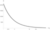Fig. 1. Electrostatic potential for simple case with zero point added: T0e = 106, T0p = 2 106.

The question now is whether this potential can ‘drag’ the protons out of the potential well of the gravitational attraction. For this, we calculated the total potential energy for protons as follows:

$$\begin{array}{c}\hfill {\stackrel{\sim }{E}}_{\mathrm{p}}=-a_{\mathrm{p}}\frac{1-\stackrel{\sim }{r}}{\stackrel{\sim }{r}}+\frac{q}{k{T}_{0_{\mathrm{p}}}}{\varphi }_{E_D}(\stackrel{\sim }{r})=\frac{\stackrel{\sim }{r}-1}{\stackrel{\sim }{r}}\left(\frac{a_{\mathrm{e}}{T}_{0_{\mathrm{e}}}+a_{\mathrm{p}}{T}_{0_{\mathrm{p}}}}{T_{0_{\mathrm{e}}}+T_{0_{\mathrm{p}}}}\right),\end{array}$$(9)

where ${\stackrel{\sim }{E}}_{\mathrm{p}}=E_{\mathrm{p}}/k{T}_{0_{\mathrm{p}}}$. We can now plot the total potential energy in Fig. 2.

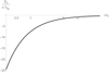Fig. 2. Total proton potential energy for simple case of two Maxwellians without magnetic field: T0e = 106, T0p = 2  ×  106.

The plot shows that he total potential energy felt by the protons is negative and monotonically increasing, resembling a purely gravitational potential. The electrostatic potential is not able to pull the protons out of the gravitational field, and they are only subject to the decreasing gravitational attraction. No finite supersonic acceleration is thus possible for the protons under the assumptions made in this section.

2.2. Proton population described by a Maxwellian distribution and electron population described by a Kappa distribution

In order to assess whether the lack of the expected maximum in the total potential energy for protons is due to the use of identical distribution functions for the two populations, we now make the same calculations as above but for two different distribution functions.

We used the same distribution for protons as in the previous section:

$$\begin{array}{c}\hfill f_{\mathrm{p}}(\mathit{r},\mathit{v})=\frac{n_{0_{\mathrm{p}}}}{{(\pi {\omega }_{0_{\mathrm{p}}})}^{(3/2)}}{e}^{-\frac{v^2}{{\omega }_{0_{\mathrm{p}}}^2}}{e}^{-\frac{R_{\mathrm{p}}(r)}{{\omega }_{0_{\mathrm{p}}}^2}},\end{array}$$

while for electrons we used the following Kappa function:

$$\begin{array}{cc}& f_{\mathrm{e}}(r,v)=\frac{n_{0_{\mathrm{e}}}}{2\pi {\left(\kappa {\omega }_{0_{\mathrm{e}}}^2\right)}^{3/2}}\frac{\mathrm{\Gamma }(\kappa +1)}{\mathrm{\Gamma }(\kappa -1/2)\mathrm{\Gamma }(3/2)}\hfill \\ \hfill & {[1+\frac{v^2+R_{\mathrm{e}}(r)}{\kappa {\omega }_{0e}^2}]}^{-(\kappa +1)},\hfill \end{array}$$(10)

where Γ(x) is the standard Gamma function, and κ is an index that shapes and gives name to the Kappa function, providing a measure of how far from the Mawellian distribution this one is (the bigger the κ value, the more the Kappa distribution approaches the Maxwellian one; see Maksimovic et al. 1997).

As in the previous case, the neutrality of the plasma imposes the equality of the densities. The calculation of the density integral for the Kappa function is slightly more complicated, but easy, since the v and r parts are still separated. After some algebraic calculations, we arrive at the following condition:

$$\begin{array}{c}\hfill n_{0_{\mathrm{p}}}{e}^{-\frac{R_{\mathrm{p}}(r)}{{\omega }_{0_{\mathrm{p}}}^2}}=n_{0_{\mathrm{e}}}{[1+\frac{R_{\mathrm{e}}(r)}{\kappa {\omega }_{0e}^2}]}^{-(\kappa +1/2)},\end{array}$$

which translates, using the same dimensionless parameters as in the previous section, to the following:

$$\begin{array}{c}\hfill e^{-(-a_{\mathrm{p}}\frac{1-\stackrel{\sim }{r}}{\stackrel{\sim }{r}}+\frac{T_{0_{\mathrm{e}}}}{T_{0_{\mathrm{p}}}}{\stackrel{\sim }{\varphi }}_E)}={(1-\frac{a_{\mathrm{e}}}{\kappa }\frac{1-\stackrel{\sim }{r}}{\stackrel{\sim }{r}}-\frac{1}{\kappa }{\stackrel{\sim }{\varphi }}_E)}^{-(\kappa +1/2)},\end{array}$$

where for simplicity we now also define a dimensionless electric potential as

$$\begin{array}{c}\hfill {\stackrel{\sim }{\varphi }}_E(\stackrel{\sim }{r})=\frac{q}{k{T}_{0_{\mathrm{e}}}}{\varphi }_E(\stackrel{\sim }{r}).\end{array}$$(11)

This deceptively simple equation can’t be solved in terms of elementary functions, and it has traditionally been solved numerically. However, a solution in terms of the transcendental Lambert function (see Appendix) can be found. The solution for the electrostatic potential is

$$\begin{array}{c}\hfill s{\stackrel{\sim }{\varphi }}_E(\stackrel{\sim }{r})=\kappa -a_{\mathrm{e}}\frac{1-\stackrel{\sim }{r}}{\stackrel{\sim }{r}}+\frac{1-2\kappa }{2}\frac{T_{0_{\mathrm{p}}}}{T_{0_{\mathrm{e}}}}W(\xi ),\end{array}$$(12)

where W(ξ) is the Lambert function of its argument, and ξ is

$$\begin{array}{cc}& \xi =\frac{2\kappa }{2\kappa -1}\frac{T_{0_{\mathrm{e}}}}{T_{0_{\mathrm{p}}}}\hfill \\ \hfill & \mathrm{Exp}\left[\frac{2}{1-2\kappa }\left[\frac{-a_{\mathrm{e}}(\stackrel{\sim }{r}-1)T_{0_{\mathrm{e}}}-a_{\mathrm{p}}(\stackrel{\sim }{r}-1)T_{0_{\mathrm{p}}}-\stackrel{\sim }{r}\kappa T_{0_{\mathrm{e}}}}{\stackrel{\sim }{r}{T}_{0_{\mathrm{p}}}}\right]\right].\hfill \end{array}$$(13)

This provides an analytic form of the electrostatic potential not found before in the literature, and it constitutes one of the main results of this paper. As in the previous case, we can calculate the electrostatic potential at the surface by making the total potential tend to zero at infinity. The limit in this case is

$$\begin{array}{c}\hfill {\stackrel{\sim }{\varphi }}_E(\stackrel{\sim }{r_0})=\kappa +a_{\mathrm{e}}+W({\xi }_{\infty }),\end{array}$$

with

$$\begin{array}{c}\hfill {\xi }_{\infty }\equiv \frac{2\kappa }{2\kappa -1}\frac{T_{0_{\mathrm{e}}}}{T_{0_{\mathrm{p}}}}\mathrm{Exp}\left[\frac{2}{1-2\kappa }\frac{-a_{\mathrm{e}}{T}_{0_{\mathrm{e}}}-a_{\mathrm{p}}{T}_{0_{\mathrm{p}}}-\kappa T_{0_{\mathrm{e}}}}{T_{0_{\mathrm{p}}}}\right].\end{array}$$

The total potential energy can be computed now:

$$\begin{array}{c}\hfill {\stackrel{\sim }{E}}_{T_{\mathrm{p}}}(\stackrel{\sim }{r})=-a_{\mathrm{p}}\frac{1-\stackrel{\sim }{r}}{\stackrel{\sim }{r}}+\frac{T_{0_{\mathrm{e}}}}{T_{0_{\mathrm{p}}}}{\stackrel{\sim }{\varphi }}_{E_{\mathrm{e}}}(\stackrel{\sim }{r}),\end{array}$$

of which the result is

$$\begin{array}{c}\hfill {\stackrel{\sim }{E}}_{T_{\mathrm{p}}}(\stackrel{\sim }{r})=(-a_{\mathrm{p}}-a_{\mathrm{e}}\frac{T_{0_{\mathrm{e}}}}{T_{0_{\mathrm{p}}}})\left(\frac{1-\stackrel{\sim }{r}}{\stackrel{\sim }{r}}\right)+\kappa \frac{T_{0_{\mathrm{e}}}}{T_{0_{\mathrm{p}}}}+\frac{1-2\kappa }{\kappa }W(\xi ),\end{array}$$(14)

where again W(ξ) is the Lambert function and ξ is given by Eq. (2.2).

We can represent the total potential energy for protons, as we did in previous the section, for T_0e = 10⁶, T_0p = 2  ×  10⁶ and now with κ = 2.5. The new obtained potential (in orange) can be compared with the one in Fig. 2 (in black). This can be seen in Fig. 3, which shows that this potential is only slightly different from the one in the previous case where two Maxwellians were assumed for the proton and electron populations.

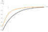Fig. 3. Total potential energy for protons, for two Maxwellians (black) and one Maxwellian and one Kappa (orange), without magnetic field: κ = 2.5, T0e = 106, T0p = 2  ×  106.

We are therefore led to conclude that the choice of different isotropic velocity distribution functions for protons and electrons, in the absence of a magnetic field, does not produce a non-monotonic potential as required for a finite acceleration of the protons.

3. Introduction of the magnetic field

In the previous sections, the magnetic field does not appear in the potential part nor in the distribution functions. This is due to the fact that we have been using fully symmetrical (or isotropic) distribution functions in the v-space. Although assuming isotropic distributions for the ions at the bottom boundary is not unreasonable, as a higher level of collisionality is expected below the exobase and down to the Sun surface (see beginning of Sect. 2), as soon as the flow becomes collisionless, in the presence of a magnetic field the v-space direction is preferred, which is dictated by the direction of the field. With a radially outward-pointing magnetic field, there would be a separation of the parallel and perpendicular velocities, and hence the peculiar trajectories of the particles within a magnetic field.

However, as we indicate in previous sections, the bulk plasma properties described by a distribution function are independent of the trajectory of its particles. Therefore, the presence of the magnetic field must somehow modify the distribution function.

A common way to formulate a distribution function that separates the parallel and perpendicular velocities is to use the so-called bi-Maxwellian and bi-Kappa functions. These functions completely separate not only the v-space component of the distribution function but also the initial temperatures, making them different for protons and electrons, resulting in eventual different parallel and perpendicular temperatures throughout the flow (unsurprisingly since they are postulated as different from the beginning). Besides that, bi-Maxwellian and bi-Kappa functions can represent proper flows when distributions are not subject to external forces.

However, our particles are flowing in a system under potential forces, both electrostatic and gravitational, and thus both must find their place in the distribution function without the necessity of artificially introducing an anisotropy in the parallel and perpendicular components, as exemplified in Meyer-Vernet (2007):

[...] “And still worse, the conditions for the distribution to be anisotropic Maxwellian (bi-Maxwellian) are difficult to realise: there must be enough collisions to produce Maxwellians in both the parallel and perpendicular directions, but not so many that the parallel and perpendicular temperatures become equal” [...],

which would be extremely difficult to attain in an environment which, by initial assumption, is considered collisionless.

We therefore had to seek a distribution function that can represent the flow of a population of protons and electrons in a magnetic field but without an anisotropy imposed externally. To that end, we considered the general form of a distribution function according to the Liouville theorem (Balescu 1975):

$$\begin{array}{c}\hfill f(v,r)=A{e}^{-\frac{E}{k{T}_0}},\end{array}$$

where E is the total energy, and therefore the normalisation constant A will have to be extracted form the overall distribution function containing the whole potential part (including the r-dependence), and not only from the v-dependent one.

We assume a radial magnetic field of the following form:

$$\begin{array}{c}\hfill \mathit{B}=\frac{B_0}{r^2}\frac{\mathit{r}}{|\mathit{r}|},\end{array}$$

and we write the distribution function as an exponential of the total energy in dimensionless units:

$$\begin{array}{cc}& f(v,r)=A\mathrm{Exp}\left[\frac{-\frac{1}{2}m{v}^2+m[{\varphi }_G(r)-{\varphi }_G(r_0)]+q[{\varphi }_E(r)-{\varphi }_E(r_0)]}{k{T}_0}\right],\hfill \\ \hfill & =A\mathrm{Exp}\left[\frac{-\frac{1}{2}m(V_{||}^2+V_{\perp }^2)+m[{\varphi }_G(r)-{\varphi }_G(r_0)]+q[{\varphi }_E(r)-{\varphi }_E(r_0)]}{k{T}_0}\right],\hfill \end{array}$$

where we have only decomposed the velocity in its parallel and perpendicular components, as can be done with any arbitrary vector.

Now we can take into account the conservation of the magnetic moment:

$$\begin{array}{c}\hfill \mu \equiv \frac{1}{2}m\frac{v_{\perp }^2}{B(r)},\end{array}$$

which implies the following:

$$\begin{array}{c}\hfill \frac{1}{2}m\frac{v_{\perp }^2}{B(r)}=\frac{1}{2}m\frac{v_{{\perp }_0}^2}{B(r_0)},\end{array}$$

assuming a magnetic field directed radially outwards and decreasing with the inverse of the square of the distance (Maksimovic et al. 1997), then we obtain

$$\begin{array}{c}\hfill B(r)=\frac{B(r_0)}{{\left(\frac{r}{r_0}\right)}^2};\end{array}$$

so, substituting the previous equality from the conservation of the magnetic field, we obtain the following:

$$\begin{array}{c}\hfill v_{\perp }^2=\frac{r_0}{r}{v}_{{\perp }_0}^2.\end{array}$$

This is very important with regard to our final results. It shows the coupling between the v and the r spaces, complicating the computation of the different integrals and ensuring that the shape of the moments of the distribution function do not all have the same r-dependency as the potential part.

With this, the distribution function now becomes

$$\begin{array}{cc}& f(r,v)=\hfill \\ \hfill & A\mathrm{Exp}\left[\frac{-\frac{1}{2}m(V_{||}^2+\frac{r_0}{r}{v}_{{\perp }_0}^2+m[{\varphi }_G(r)-{\varphi }_G(r_0)]+q[{\varphi }_E(r)-{\varphi }_E(r_0)]}{k{T}_0}\right].\hfill \end{array}$$

Now we affirm that for r = r₀ we should obtain the initial function that should be normalised to the total density. When we have r = r_0, we should recover the initial function:

$$\begin{array}{c}\hfill f(v,r_0)=A{e}^{\frac{(1/2)m{v}_0^2}{k{T}_0}},\end{array}$$

whether v is decomposed in parallel and perpendicular parts or not. Therefore, the constant of normalisation is the same as the one with only a v part, and therefore

$$\begin{array}{c}\hfill f(v,r)=\frac{n_0}{{\pi }^{3/2}{(\frac{2k{T}_0}{m})}^{(3/2)}}{e}^{\frac{-\frac{1}{2}m(V_{||}^2+\frac{r_0}{r}{v}_{{\perp }_0}^2+m[{\varphi }_G(r)-{\varphi }_G(r_0)]+q[{\varphi }_E(r)-{\varphi }_E(r_0)]}{k{T}_0}},\end{array}$$

where T₀ is the initial temperature, and the temperature throughout the flow is obtained through the moments of the distribution function.

The same reasoning can be applied to the Kappa function: the constant for the overall distribution function with the potential part can only be extracted from the initial condition that the initial distribution function at r = r₀ has to be normalised. Therefore, to find this normalisation constant, we look for the following:

$$\begin{array}{c}\hfill f_{\kappa }(v)=A_{\kappa }{(1+\frac{(1/2)m{v}^2}{\kappa kT})}^{-(\kappa +1)};\end{array}$$

thus, integrating over the full volume we obtain $\int f(\mathit{v}){\mathrm{d}}^3\mathit{v}=4\pi {\int }_0^{\infty }{f}_{\kappa }(\mathit{v}){\mathit{v}}^2\mathrm{d}\mathit{v}=n_0,$ and from here we obtain

$$\begin{array}{c}\hfill A_{\kappa }=\frac{n_0}{{\left(\frac{2\pi k{T}_0\kappa }{m}\right)}^{(3/2)}}\frac{\mathrm{\Gamma }(\kappa +1)}{\mathrm{\Gamma }(\kappa -1/2)};\end{array}$$

so, the Kappa function without the magnetic field would finally be written as follows:

$$\begin{array}{c}\hfill f_{\kappa }(v)=\frac{n_0}{{\left(\frac{2\pi k{T}_0\kappa }{m}\right)}^{(3/2)}}\frac{\mathrm{\Gamma }(\kappa +1)}{\mathrm{\Gamma }(\kappa -1/2)}{(1+\frac{(1/2)m{v}^2}{\kappa kT})}^{-(\kappa +1)}.\end{array}$$

In summary, the two distribution functions including the potential part that we use henceforth are the following:

$$\begin{array}{cc}& f_{\mathrm{p}}(r,v)=\frac{n_0}{{({\omega }_{0_{\mathrm{p}}}\sqrt{\pi })}^3}\mathrm{Exp}[-\frac{v_{\mathrm{p}}^2+R_{\mathrm{p}}(r)}{{\omega }_{0_{\mathrm{p}}}^2}],\hfill \end{array}$$(15)

$$\begin{array}{cc}\hfill & f_{e(r,v)}=\frac{n_0}{{({\omega }_{0_{\mathrm{e}}}\sqrt{\pi })}^3}\frac{\mathrm{\Gamma }(\kappa +1)}{\mathrm{\Gamma }(\kappa -1/2)}{[1+\frac{v_{\mathrm{e}}^2+R_{\mathrm{e}}(r)}{\kappa {\omega }_{0_{\mathrm{e}}}^2}]}^{-(\kappa +1)},\hfill \end{array}$$(16)

whereas before,

$$\begin{array}{cc}& \frac{R_{\mathrm{p}}(r)}{{\omega }_{0_{\mathrm{p}}}^2}=-a_{\mathrm{p}}\frac{1-\stackrel{\sim }{r}}{\stackrel{\sim }{r}}+\frac{T_{0_{\mathrm{e}}}}{T_{0_{\mathrm{p}}}}{\stackrel{\sim }{\varphi }}_E(\stackrel{\sim }{r})\hfill \\ \hfill & \frac{R_{\mathrm{e}}(r)}{{\omega }_{0_{\mathrm{e}}}^2}=-a_{\mathrm{e}}\frac{1-\stackrel{\sim }{r}}{\stackrel{\sim }{r}}-{\stackrel{\sim }{\varphi }}_E(\stackrel{\sim }{r}).\hfill \end{array}$$

We later show that the election of the normalisation constant will only have a quantitative effect on the results, but will not modify the overall shape of the potential energy.

3.1. One Maxwellian and one Kappa with magnetic field

For the calculation of the density integrals, we now have to take into account that the v and r spaces are coupled via the presence of the magnetic moment conservation. The spherical symmetry disappears, and cylindrical coordinates are more appropriate where the total density would be calculated from

$$\begin{array}{c}\hfill n_{\mathrm{total}}={\displaystyle \int }f(v,r){\mathrm{d}}^{3}v={\displaystyle {\int }_{-\infty }^{\infty }\mathrm{d}{v}_{\Vert }{\int }_0^{\infty }2\pi v_{\perp }\mathrm{d}{v}_{\perp }f(v_{\Vert },v_{\perp },r).}\end{array}$$

This total density is calculated over the whole velocity space. Since the velocity space is now coupled to the r space via the conservation of the magnetic moment, the density will depend on r in a non-trivial form. In the limit when r → ∞,  we should recover the total density over the whole space. Therefore, the r-dependent density will come from the following integrals:

$$\begin{array}{c}\hfill n(r)={\displaystyle {\int }_{-\infty }^{\infty }\mathrm{d}{v}_{\Vert }{\int }_0^{v_{\perp }(r)}2\pi v_{\perp }^{\prime }\mathrm{d}{v}_{\perp }^{\prime }f(v_{\Vert },v_{\perp }^{\prime },r),}\end{array}$$

where the prime in the perpendicular velocity is included to make the dummy variable explicit, but it will be dropped in the subsequent formulae. This density should equal the total density in the limit when v_⊥ → ∞. Therefore, for the r-dependent density we obtain the following:

$$\begin{array}{c}\hfill n(r)={\displaystyle {\int }_{-\infty }^{\infty }\mathrm{d}{v}_{\Vert }{\int }_{\infty }^{v_{\perp 0}{r}_0/r}-2\pi (v_{{\perp }_0}/r)(v_{{\perp }_0}/r^2)\mathrm{d}r{f}_{M_i}(v_{\Vert },r).}\end{array}$$

With some algebra, we finally obtain the following formula for the density for protons:

$$\begin{array}{c}\hfill n_{\mathrm{p}}(r)=-\frac{2v_{{\perp }_0}^2{n}_{0_{\mathrm{p}}}}{{\omega }_0^2}{\displaystyle {\int }_{\infty }^{v_{\perp 0}{r}_0/r}\frac{\mathrm{d}r}{r^3}{e}^{-(v_{{\perp }_0}^2{r}_0/r^2+R_{\mathrm{p}}(r))/{\omega }_0^2},}\end{array}$$

and using the same dimensional parameters as in the previous case, we attain the following:

$$\begin{array}{c}\hfill n_{\mathrm{p}}(\stackrel{\sim }{r})=-\frac{2v_{{\perp }_{0_{\mathrm{p}}}}^2{n}_0}{{\omega }_0^2}{\displaystyle {\int }_{\infty }^{v_{\perp 0_{\mathrm{p}}}/\stackrel{\sim }{r}}\frac{\mathrm{d}\stackrel{\sim }{r}}{{\stackrel{\sim }{r}}^3}{e}^{-{\left(\frac{v_{{\perp }_{0_{\mathrm{p}}}}}{{\omega }_{0_{\mathrm{p}}}\stackrel{\sim }{r}}\right)}^2}{e}^{-a_{\mathrm{p}}\frac{1-\stackrel{\sim }{r}}{\stackrel{\sim }{r}}}{e}^{-\frac{T_{0_{\mathrm{e}}}}{T_{0_{\mathrm{p}}}}{\stackrel{\sim }{\varphi }}_{E_{\mathrm{e}}}(\stackrel{\sim }{r})}.}\end{array}$$(17)

We can similarly calculate the density integral for the electrons to finally yield

$$\begin{array}{cc}& n_{\mathrm{e}}(\stackrel{\sim }{r})=-2\sqrt{\kappa }{v}_{{\perp }_{0_{\mathrm{e}}}}^2\frac{n_{0_{\mathrm{e}}}}{{\omega }_{0_{\mathrm{e}}}^2}\frac{\mathrm{\Gamma }(\kappa +1)}{\mathrm{\Gamma }(\kappa -1/2)}\hfill \\ \hfill & {\displaystyle {\int }_{\infty }^{v_{\perp 0_{\mathrm{e}}}/\stackrel{\sim }{r}}\frac{\mathrm{d}\stackrel{\sim }{r}}{{\stackrel{\sim }{r}}^3}[1+\frac{1}{\kappa {\omega }_{0_{\mathrm{e}}}^2}{\left(\frac{v_{\perp 0_{\mathrm{e}}}}{\stackrel{\sim }{r}}\right)}^2+\frac{1}{\kappa }\left(a_{\mathrm{e}}\frac{1-\stackrel{\sim }{r}}{\stackrel{\sim }{r}}\right)-{\stackrel{\sim }{\varphi }}_{E_{\mathrm{e}}}(\stackrel{\sim }{r})].}\hfill \end{array}$$(18)

The equality of densities thus implies the following:

$$\begin{array}{cc}& -\frac{2v_{{\perp }_{0_{\mathrm{p}}}}^2{n}_{0_{\mathrm{p}}}}{{\omega }_0^2}{\displaystyle {\int }_{\infty }^{v_{\perp 0_{\mathrm{p}}}/\stackrel{\sim }{r}}\frac{\mathrm{d}\stackrel{\sim }{r^{\prime }}}{{\stackrel{\sim }{r}}^{\prime 3}}{e}^{-{\left(\frac{v_{{\perp }_{0_{\mathrm{p}}}}}{{\omega }_{0_{\mathrm{p}}}\stackrel{\sim }{r^{\prime }}}\right)}^2}{e}^{a_{\mathrm{p}}\frac{1-\stackrel{\sim }{r^{\prime }}}{\stackrel{\sim }{r^{\prime }}}}{e}^{-\frac{T_{0_{\mathrm{e}}}}{T_{0_{\mathrm{p}}}}{\stackrel{\sim }{\varphi }}_{E_{\mathrm{e}}}}}\hfill \\ \hfill & =-2\sqrt{\kappa }{v}_{{\perp }_{0_{\mathrm{e}}}}^2\frac{n_{0_{\mathrm{e}}}}{{\omega }_{0_{\mathrm{e}}}^2}\frac{\mathrm{\Gamma }(\kappa +1)}{\mathrm{\Gamma }(\kappa -1/2)}\hfill \\ \hfill & {\displaystyle {\int }_{\infty }^{v_{\perp 0_{\mathrm{e}}}/\stackrel{\sim }{r}}\frac{\mathrm{d}\stackrel{\sim }{r^{\prime }}}{{\stackrel{\sim }{r^{\prime }}}^3}[1+\frac{1}{\kappa {\omega }_{0_{\mathrm{e}}}^2}{\left(\frac{v_{\perp 0_{\mathrm{e}}}}{\stackrel{\sim }{r^{\prime }}}\right)}^2+\frac{1}{\kappa }(-a_{\mathrm{e}}\frac{1-\stackrel{\sim }{r^{\prime }}}{\stackrel{\sim }{r^{\prime }}})-{\stackrel{\sim }{\varphi }}_{E_{\mathrm{e}}}],}\hfill \end{array}$$

where the prime in the integrands $\stackrel{\sim }{r^{\prime }}$ is there to emphasise its dummy character.

It can now be demonstrated that given two integrals,

$$\begin{array}{cc}& I_1={\displaystyle {\int }_{\infty }^{a/u}f(x)\mathrm{d}x}\hfill \\ \hfill & I_2={\displaystyle {\int }_{\infty }^{b/u}g(x)\mathrm{d}x,}\hfill \end{array}$$

a solution of the equation I₁ = I₂ is given by af(x) = bg(x), and therefore we have the following equation for the equality of densities:

$$\begin{array}{cc}& \frac{2v_{{\perp }_{0_{\mathrm{p}}}}^3}{{\omega }_0^2}{n}_{0_{\mathrm{p}}}{e}^{-{\left(\frac{v_{{\perp }_{0_{\mathrm{p}}}}}{{\omega }_{0_{\mathrm{p}}}\stackrel{\sim }{r^{\prime }}}\right)}^2}{e}^{a_{\mathrm{p}}\frac{1-\stackrel{\sim }{r^{\prime }}}{\stackrel{\sim }{r^{\prime }}}}{e}^{-\frac{T_{0_{\mathrm{e}}}}{T_{0_{\mathrm{p}}}}{\stackrel{\sim }{\varphi }}_{E_{\mathrm{e}}}}\hfill \\ \hfill & =\sqrt{\kappa }\frac{v_{{\perp }_{0_{\mathrm{e}}}}^3}{{\omega }_{0_{\mathrm{e}}}^2}{n}_{0_{\mathrm{e}}}\frac{\mathrm{\Gamma }(\kappa +1)}{\mathrm{\Gamma }(\kappa -1/2)}[1+\frac{1}{\kappa {\omega }_{0_{\mathrm{e}}}^2}{\left(\frac{v_{\perp 0_{\mathrm{e}}}}{\stackrel{\sim }{r^{\prime }}}\right)}^2+\frac{1}{\kappa }(-a_{\mathrm{e}}\frac{1-\stackrel{\sim }{r^{\prime }}}{\stackrel{\sim }{r^{\prime }}})-{\stackrel{\sim }{\varphi }}_{E_{\mathrm{e}}}].\hfill \end{array}$$

The solution to this equation can again be given in terms of the Lambert function:

$$\begin{array}{c}\hfill {\stackrel{\sim }{\varphi }}_{E_{\mathrm{e}}}(\stackrel{\sim }{r})=\kappa -a_{\mathrm{e}}\frac{1-\stackrel{\sim }{r}}{\stackrel{\sim }{r}}+\frac{v_{{\perp }_{0_{\mathrm{e}}}}^2}{{\omega }_{0_{\mathrm{e}}}^2{\stackrel{\sim }{r}}^2}\frac{1-2\kappa }{2}\frac{T_{0_{\mathrm{p}}}}{T_{0_{\mathrm{e}}}}W(\xi ),\end{array}$$(19)

with the argument being

$$\begin{array}{c}\hfill \xi =\frac{2\kappa }{2\kappa -1}\frac{T_{0_{\mathrm{e}}}}{T_{0_{\mathrm{p}}}}{e}^{{\left[\frac{(-a_{\mathrm{p}}-a_{\mathrm{e}}\frac{T_{0_{\mathrm{e}}}}{T_{0_{\mathrm{p}}}})\left(\frac{\stackrel{\sim }{r}-1}{\stackrel{\sim }{r}}\right)-\frac{1}{{\stackrel{\sim }{r}}^2}(\frac{T_{0_{\mathrm{e}}}}{T_{0_{\mathrm{p}}}}\frac{v_{{\perp }_{0_{\mathrm{e}}}}^2}{{\omega }_{0_{\mathrm{e}}}^2}+\frac{v_{{\perp }_{0_{\mathrm{p}}}}^2}{{\omega }_{0_{\mathrm{p}}}^2})-\frac{T_{0_{\mathrm{e}}}}{T_{0_{\mathrm{p}}}}\kappa }{\stackrel{\sim }{r}{T}_{0_{\mathrm{p}}}}\right]}^{\frac{2}{1-2\kappa }}}.\end{array}$$

It is worth noting that this solution is practically identical to the previous case in Sect. 2.2 with the exception of the appearance of a term in $1/{\stackrel{\sim }{r}}^2$ and of course the presence of the initial perpendicular velocities. The total potential for the protons can now be obtained as before, making

$$\begin{array}{c}\hfill {\stackrel{\sim }{E}}_{\mathrm{p}}(\stackrel{\sim }{r})=-a_{\mathrm{p}}\frac{1-\stackrel{\sim }{r}}{\stackrel{\sim }{r}}+\frac{T_{0_{\mathrm{e}}}}{T_{0_{\mathrm{p}}}}{\stackrel{\sim }{\varphi }}_{E_{\mathrm{e}}}(\stackrel{\sim }{r}).\end{array}$$

The result of this calculation and its interpretation are given in the next sub-section.

3.2. Interpretation of the solution

Now we can plot the analytic solution for the total potential for protons for different values of the parameters κ, v_⊥0e, v_⊥0p, T_0e, T_0p. For instance, for κ = 2.5, v_⊥0e = 0.1ω_0e, v_⊥0p = 0.4ω_0p, T_0e = 10⁶, T_0p = 2 × 10⁶ the total potential can be represented as in Fig. 4.

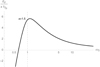Fig. 4. Total potential energy of protons for a Maxwellian distribution for protons and a Kappa for electrons with magnetic field, κ = 2.5, v⊥0e = 0.1ω0e, v⊥0p = 0.4ω0p, T0e = 106, T0p = 2.106.

It can now be seen that the total potential energy for protons changes its shape and is no longer monotonic. The protons are initially experiencing a decelerating total potential until a maximum is reached. We thus found a similar situation to that of Zouganelis et al. (2004), suggesting a stronger acceleration compared to the previous section. We note that all potential plots only have a physical meaning at an altitude above one solar radius (i.e. surface of the Sun). This altitude is marked on the plot with the vertical dashed line at r = 1.

The different behaviour of this solution with respect to the similar one in the previous case with no magnetic field is due to the $1/{\stackrel{\sim }{r}}^2$ term that is directly related to the existence of the magnetic field through the magnetic moment conservation. The closer the initial perpendicular velocities are to zero, the more the potential approaches a monotonically decreasing potential. The initial perpendicular velocities of the particles thus play a crucial role in the appearance of the acceleration in our model. This is not surprising, since this affects the parallel velocities when applying the conservation of energy and magnetic moment.

We now plot the total potential energy for different values of kappa in Fig. 5, which shows that the increasing value of kappa approximates the case where the potential is monotonically increasing, as was the case in Sect. 2.1. This matches the fact that the Kappa distribution approaches the Maxwellian as kappa increases.

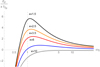Fig. 5. Total potential energy of protons for a Maxwellian for protons and a Kappa for electrons with magnetic field for different kappa values: v⊥0e = 0.1ω0e, v⊥0p = 0.4ω0p, T0e = 106, T0p = 2 × 106.

The total potential energy for different initial proton temperatures can also be calculated and is shown in Fig. 6. For equal initial proton and electron temperatures, the shape of the potential energy does not show a maximum (black line), while increasing the initial proton temperature produces the expected maximum to obtain the required shape for the acceleration. This is in agreement with any fluid Parker-type model that produces a higher acceleration for a higher initial proton temperature.

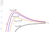Fig. 6. Total potential energy of protons for a Maxwellian distribution for protons and a Kappa for electrons with magnetic field for different proton temperature values: κ = 2.5, v⊥0e = 0.1ω0e, v⊥0p = 0.4ω0p, T0e = 106.

Finally, we plot the case for varying initial proton perpendicular initial velocity in Fig. 7.

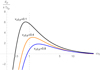Fig. 7. Total potential energy for protons for a Maxwellian for protons and a Kappa for electrons with magnetic field for different proton initial perpendicular velocity values: κ = 2.5, v⊥0e = 0.1ω0e, T0e = 106, T0p = 2 × 106.

4. Conclusions

Via simple assumptions on the flow of the particles within the solar wind, we find an analytic solution of the electrostatic potential of the solar wind valid for all r distances. This solution is given in terms of the Lambert function.

The solution found for the total potential energy is similar to the one given in the most advanced exospheric models (see Zouganelis et al. 2004) where different methods are used. In the standard exospheric models, the presence of the magnetic field is forced into the moment calculations from the distribution functions – via the different particle trajectories – and the consequent use of so-called truncated distributions. In this new approach, the presence of the magnetic field is included in the distribution functions through the conservation of the magnetic moment.

Both methods make use of kinetic collisionless equations for the plasma, albeit in different ways, and thus the similarity in their solutions is reasonable. The final solution in this new approach depends on the initial perpendicular velocities; if those are zero, the presence of the magnetic field in the distributions disappears and the non-monotonic profile of the total potential is not produced. The selection of the normalisation constant for the distributions is only made based on the normalisation of the functions at the surface of the Sun r₀.

The method followed to find our solution can be used verbatim for other Kappa functions with different normalisations without much difficulty. The presence of those different normalisation factors will only change the numbers quantitatively, but will not qualitatively change the shape of the potentials.

In our method, we did not have to make any assumption on the initial electrostatic potential at the surface of the Sun. We calculate it by imposing that it be zero at infinity. The initial perpendicular velocities have been taken as fractions of the thermal velocity for each particle species.

Compared to the standard exospheric approach, our result provides a solution that (a) does not require assumptions on the particle populations as in exospheric models (ballistic, escaping, trapped), (b) does not require truncated functions, and (c) avoids the inconsistency of the trapped particles. Trapped particles appear in exospheric models for particles that do not have enough energy to escape from the gravitational field, but they do not fall back to the Sun as they are magnetically reflected because of their large pitch angles. In principle, these models demonstrate an inconsistency, as these particles should not exist in the pure absence of collisions. At the same time, in exospheric models the absence of trapped particles leads to a subsonic wind, making their presence necessary. In the present approach, this inconsistency disappears, as the distribution functions are uniformly populated without any discontinuities.

It is important to note that this approach, as the exospheric one, is not meant to reproduce the solar wind properties as a sophisticated 3D model would do. It is, however, useful to give us insight on the dependence of the acceleration as a function of the non-thermal properties of the electrons (i.e. as a function of kappa). The lower the kappa, the stronger the acceleration, suggesting that the shape of the electron distributions at the corona or even lower may play a preponderant role in the acceleration of the solar wind. It is obvious that other complex processes play their own part on solar wind physics, but the present model can help us identify the relative importance of the role of the velocity filtration due to the non-thermal properties of the electrons. In particular, they can give hints to explain electron properties as observed in the inner heliosphere by Helios (Berčič et al. 2019) and the Parker Solar Probe (Moncuquet et al. 2020; Martinović et al. 2020; Maksimovic et al. 2020; Halekas et al. 2020). As the Solar Orbiter (Müller et al. 2020) and Parker Solar Probe get closer to the Sun, the non-thermal properties of the electrons will be further detailed and extrapolated down to the corona and to the base of the wind. If non-thermal electrons do exist at the corona, the present model can successfully account for their role in the acceleration of the solar wind.

Acknowledgments

Javier Rodríguez-Pacheco acknowledges Spanish Ministerio de Ciencia, Innovación y Universidades for grant PID2019- 104863RB-I00/AEI/10.13039/501100011033

References

Appendix A: Lambert function

The Lambert function, which we call W, is the solution to the following equation:

$$\begin{array}{c}\hfill W{e}^W=x,\end{array}$$(A.1)

where by ‘solution’ we actually mean the ‘inverse’ solution, meaning the values of W for given x values. This is similar to saying that U is the inverse solution of the following equation:

$$\begin{array}{c}\hfill e^U=x,\end{array}$$

which is more familiar and intimately related to the Lambert function. The W function is only defined for certain arguments in the real plane, as is the U function (result of the exponential equation) since the natural logarithms are only defined in the positive x-axis. It can be extended, as can the logarithms, to the complex plane, but in this paper we are only concerned with its real values, which go from −1/e ≤ x ≤ ∞. The function equals -1 for x = −1/e and tends slowly towards infinity with x → ∞.

A representation of the W Lambert function can be seen in Figure A.1, and its close relation with the logarithm function can be seen in Figure A.2.

The Lambert function cannot be expressed in terms of elementary functions, and thus it is said to be ’transcendental’. It was first mentioned by Johann Heinrich Lambert as part of another set of transcendental equations in 1758, and it was then given its name by Leonhard Euler, who specifically discussed the above function in a paper in 1783.

The Lambert equation can be derived, and thus a derivative of the Lambert function is obtained as follows:

$$\begin{array}{c}\hfill W^{\prime }(x)=\frac{W(x)}{x(1+W(x))}.\end{array}$$

A primitive can also be found for this function to be

$$\begin{array}{c}\hfill {\displaystyle \int }xW(x)dx=x(W(x)-1+\frac{1}{W(x)})+C.\end{array}$$

Despite having received little attention from the science community since its inception in the late 18th century, the Lambert function is more ubiquitous than may be initially assumed. A good set of examples can be found in Corless & Gonnet (1996).

Since some years ago, several mathematical tools have added support for the Lambert function to their software. This work made use of the implementation of the Lambert function in the Mathematica software (Wolfram 2019). Explicit information on how it makes use of the function can be found in Weisstein (2019).

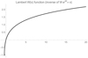Fig. A.1. Real branch of the Lambert function W(x).

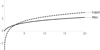Fig. A.2. Lambert and log functions.

All Figures

	Fig. 1. Electrostatic potential for simple case with zero point added: T0e = 106, T0p = 2 106.
In the text

	Fig. 2. Total proton potential energy for simple case of two Maxwellians without magnetic field: T0e = 106, T0p = 2  ×  106.
In the text

	Fig. 3. Total potential energy for protons, for two Maxwellians (black) and one Maxwellian and one Kappa (orange), without magnetic field: κ = 2.5, T0e = 106, T0p = 2  ×  106.
In the text

	Fig. 4. Total potential energy of protons for a Maxwellian distribution for protons and a Kappa for electrons with magnetic field, κ = 2.5, v⊥0e = 0.1ω0e, v⊥0p = 0.4ω0p, T0e = 106, T0p = 2.106.
In the text

	Fig. 5. Total potential energy of protons for a Maxwellian for protons and a Kappa for electrons with magnetic field for different kappa values: v⊥0e = 0.1ω0e, v⊥0p = 0.4ω0p, T0e = 106, T0p = 2 × 106.
In the text

	Fig. 6. Total potential energy of protons for a Maxwellian distribution for protons and a Kappa for electrons with magnetic field for different proton temperature values: κ = 2.5, v⊥0e = 0.1ω0e, v⊥0p = 0.4ω0p, T0e = 106.
In the text

	Fig. 7. Total potential energy for protons for a Maxwellian for protons and a Kappa for electrons with magnetic field for different proton initial perpendicular velocity values: κ = 2.5, v⊥0e = 0.1ω0e, T0e = 106, T0p = 2 × 106.
In the text

	Fig. A.1. Real branch of the Lambert function W(x).
In the text

	Fig. A.2. Lambert and log functions.
In the text

References

- Balescu, R. 1975, Equilibrium and Non-Equilibrium Statistical Mechanics, 1, 109 [Google Scholar]
- Berčič, L., Maksimović, M., Landi, S., & Matteini, L. 2019, MNRAS, 486, 3404 [Google Scholar]
- Chamberlain, J. W. 1960, ApJ, 131, 47 [NASA ADS] [CrossRef] [Google Scholar]
- Corless, R., & Gonnet, G. 1996, Adv. Comput. Math., 5, 329 [CrossRef] [MathSciNet] [Google Scholar]
- Cranmer, S. R., Gibson, S. E., & Riley, P. 2017, Space Sci. Rev., 212, 1345 [Google Scholar]
- Echim, M., Lemaire, J., & Lie-Svendsen, O. 2011, Surv. Geophys., 1, 70 [NASA ADS] [Google Scholar]
- Halekas, J. S., Whittlesey, P., Larson, D. E., et al. 2020, ApJS, 246, 22 [Google Scholar]
- Jockers, K. 1970, A&A, 6, 19 [NASA ADS] [Google Scholar]
- Krall, N. A., & Trivelpiece, A. W. 1973, Principles of Plasma Physics, 1, 79 [NASA ADS] [Google Scholar]
- Lamy, H., Pierrard, V., Maksimovic, M., & Lemaire, J. F. 2003, J. Geophys. Res. (Space Phys.), 108, 1047 [NASA ADS] [CrossRef] [Google Scholar]
- Lemaire, J., & Scherer, M. 1971, J. Geophys. Res., 76, 7479 [Google Scholar]
- Lemaire, J., & Scherer, M. 1973, Rev. Geophys. Space Phys., 11, 427 [Google Scholar]
- Maksimovic, M., Pierrard, V., & Lemaire, J. 1997, A&A, 324, 725 [NASA ADS] [Google Scholar]
- Maksimovic, M., Bale, S. D., Berčič, L., et al. 2020, ApJS, 246, 62 [Google Scholar]
- Martinović, M. M., Klein, K. G., Kasper, J. C., et al. 2020, ApJS, 246, 30 [Google Scholar]
- Meyer-Vernet, N. 2007, Basics of the Solar Wind (Cambridge, UK: Cambridge University Press) [Google Scholar]
- Meyer-Vernet, N., & Issautier, K. 1998, J. Geophys. Res., 103, 29705 [NASA ADS] [CrossRef] [Google Scholar]
- Moncuquet, M., Meyer-Vernet, N., Issautier, K., et al. 2020, ApJS, 246, 44 [Google Scholar]
- Müller, D., St. Cyr, O. C., Zouganelis, I., et al. 2020, A&A, 642, A1 [CrossRef] [EDP Sciences] [Google Scholar]
- Parker, E. 2010, AIP Conference Proceedings, 1216 [Google Scholar]
- Pierrard, V., Issautier, K., Meyer-Vernet, N., & Lemaire, J. 2001, Geophys. Res. Lett., 28, 223 [CrossRef] [Google Scholar]
- Pierrard, V., & Lemaire, J. 1996, J. Geophys. Res., 101, 7923 [CrossRef] [Google Scholar]
- Weisstein, E. W. 2019, MathWorld-A Wolfram Web Resource, 1, https://mathworld.wolfram.com/LambertW [Google Scholar]
- Wolfram, 2019, Research,& Inc., 1 [Google Scholar]
- Zouganelis, I., Maksimovic, M., Meyer-Vernet, N., Lamy, H., & Issautier, K. 2004, ApJ, 606, 542 [Google Scholar]
- Zouganelis, I., Meyer-Vernet, N., Landi, S., Maksimovic, M., & Pantellini, F. 2005, ApJ, 626, L117 [Google Scholar]