© ESO 2021

1. Introduction

Mass is one of the most fundamental characteristics of particles and fields, and a long-standing problem in classical field theory is whether or not the graviton, the spin-2 particle that mediates gravity, can have a non-zero mass. The seminal work by Fierz & Pauli (1939) uncovered a unique Lorentz-invariant graviton mass term at the level of a linear theory. van Dam & Veltman (1970) and Zakharov (1970) found a discontinuity at the massless limit of the Fierz-Pauli theory, questioning its viability because the discontinuity would imply an 𝒪(1) deviation from general relativity (GR) however small the mass of the graviton. While the discontinuity of the massless limit can be resolved by non-linearity as shown by Vainshtein (1972), Boulware & Deser (1972, BD) in the same year pointed out that the same kind of non-linearity that saved the massive gravity from the discontinuity causes a problem, namely that there appears a ghost at the non-linear level. The BD ghost posed a problem for the massive gravity for almost 40 years until de Rham & Gabadadze (2010; dRGT) discovered a fully non-linear classical theory of massive gravity without the BD ghost.

Given a consistent non-linear theory of massive gravity, it is natural to study its implications for cosmology. In particular, as the graviton mass modifies the behaviour of gravity at long distances, it would be interesting to ask whether the modified dynamics can address the mystery of the accelerated expansion of the Universe today. However, it soon turned out that the dRGT theory does not allow an expanding (or contracting) flat Friedmann-Lemaître-Robertson-Walker (FLRW) solution (D’Amico et al. 2011). Although an open FLRW solution with self-acceleration was found (Gumrukcuoglu et al. 2011), it was shown that the solution suffers from ghost instability at the non-linear level (De Felice et al. 2012). If we extend the dRGT theory by allowing for a non-Minkowski fiducial metric, then another branch of FLRW solutions can be found. This branch is called the normal branch, in contrast to the previous one called the self-accelerating branch, and suffers from an instability at the linear level called the Higuchi ghost (Higuchi 1987; Fasiello & Tolley 2012). For these reasons, all FLRW solutions in dRGT theory (with an either Minkowski or non-Minkowski fiducial metric) are unstable (De Felice et al. 2012).

Progress has been made towards stable cosmological solutions in the framework of non-linear massive gravity. In general, there are two options: to break the symmetry of FLRW (i.e. either homogeneity (D’Amico et al. 2011) or isotropy (Gumrukcuoglu et al. 2012; De Felice et al. 2013)) or to extend the theory (see e.g. Kenna-Allison et al. 2020 and references therein).

The minimal theory of massive gravity (MTMG) (De Felice & Mukohyama 2016a,b) was built upon dRGT theory by enforcing the physical and fiducial vielbeins to be simultaneously of the Arnowitt-Deser-Misner (ADM) form and adding extra constraints to eliminate the unwanted degrees of freedom. (Minimal theory of quasidilaton massive gravity (De Felice et al. 2017a,b, 2019) is also constructed in this way upon the quasidilaton theory (D’Amico et al. 2013). As the number of gravitational degrees of freedom in MTMG is only two (corresponding to tensorial gravitational waves), the theory is free from various instabilities such as the BD ghost, the Higuchi ghost, and the non-linear ghost mentioned above, and therefore provides a stable non-linear completion of the cosmological solutions in both branches of dRGT theory. In the self-accelerating branch, the graviton mass term acts as an effective cosmological constant that accelerates the expansion of the universe and the scalar perturbations behave exactly the same as in the standard ΛCDM model of GR. Moreover, the self-accelerating branch allows for GR solutions in spherical symmetry without instabilities or extra singularities (De Felice et al. 2018). In the normal branch, on the other hand, the evolution equations for the scalar perturbations are different from those in ΛCDM and show interesting phenomenology. For example, the normal branch of MTMG may fit the redshift space distortion data better than ΛCDM (De Felice & Mukohyama 2017) without conflicting with the integrated Sachs-Wolfe-galaxy correlation data (Bolis et al. 2018). Furthermore, MTMG may provide a simple mechanism to enhance stochastic gravitational waves (Fujita et al. 2019, 2020).

The purpose of the present paper is to explore the non-linear dynamics of MTMG for the first time by performing N-body simulations. In the self-accelerating branch, the deviation from the ΛCDM model in GR is expected to be minimal (if any). In the present paper, we therefore focus on the normal branch, which exhibits an interesting deviation from ΛCDM in the form of an environment-dependent effective gravitational constant G_eff as a function of the graviton mass and the local energy density.

The remainder of the present paper is organised as follows. In Sect. 2 we briefly review MTMG and present the basic equations. After describing the implementation of the environment-dependent gravitational coupling in a modified version of the N-body code RAMSES in Sect. 3, we calibrate the best-fit value of the MTMG parameter θ taking into account the effects of voids in Sect. 4. We then explore the predictions of MTMG in the non-linear regime. In Sect. 5 we show the results of the N-body simulations in MTMG, including the power spectra, the halo mass function, the halo density profile, the halo gravitational constant profile, and the void density profile. Section 6 is then devoted to a summary of the paper and some discussions.

2. The model and its basic equations

The minimal theory of massive gravity (MTMG) introduced in De Felice & Mukohyama (2016b) is defined through the following action:

$$\begin{array}{cc}\hfill S_{\mathrm{MTMG}}& =S_{\mathrm{GR}}+\frac{M_{\mathrm{P}}^2}{2}{\displaystyle \sum _{i=1}^4\int {\mathrm{d}}^{4}x{\mathcal{S}}_i+S_{\mathrm{constr}}+S_{\mathrm{m}},}\hfill \end{array}$$(1)

$$\begin{array}{cc}\hfill {\mathcal{S}}_1& =-m^2{c}_1\sqrt{\stackrel{\sim }{\gamma }}(N+M\mathcal{K}),\hfill \end{array}$$(2)

$$\begin{array}{cc}\hfill {\mathcal{S}}_2& =-\frac{1}{2}{m}^2{c}_2\sqrt{\stackrel{\sim }{\gamma }}(2N\mathcal{K}+M{\mathcal{K}}^2-M{\stackrel{\sim }{\gamma }}^{\mathit{ij}}{\gamma }_{\mathit{ji}}),\hfill \end{array}$$(3)

$$\begin{array}{cc}\hfill {\mathcal{S}}_3& =-m^2{c}_3\sqrt{\gamma }(M+N\mathfrak{K}),\hfill \end{array}$$(4)

$$\begin{array}{cc}\hfill {\mathcal{S}}_4& =-m^2{c}_4\sqrt{\gamma }N.\hfill \end{array}$$(5)

Here, S_m denotes a general matter action and the GR part of the action is given by the well-known ADM expression

$$\begin{array}{c}\hfill S_{\mathrm{GR}}=\frac{M_{\mathrm{P}}^2}{2}{\displaystyle \int }{\mathrm{d}}^{4}xN\sqrt{\gamma }{[}^{(3)}R+K^{\mathit{ij}}{K}_{\mathit{ij}}-K^2],\end{array}$$(6)

where the following quantities represent the extrinsic curvature and its trace respectively:

$$\begin{array}{cc}\hfill K_{\mathit{ij}}& =\frac{1}{2N}({\dot{\gamma }}_{\mathit{ij}}-{\mathcal{D}}_i{N}_j-{\mathcal{D}}_j{N}_i),\hfill \end{array}$$(7)

$$\begin{array}{cc}\hfill K& ={\gamma }^{\mathit{ij}}{K}_{\mathit{ij}}.\hfill \end{array}$$(8)

Here, the fields N and Nⁱ are the lapse and shift, γ_ij is the three-dimensional spatial metric, ⁽³⁾R is the Ricci scalar of γ_ij, 𝒟_i corresponds to the covariant derivative compatible with γ_ij, and γ ≡ detγ_ij. In the above expressions, we have also the Planck mass squared, $M_{\text{P}}^2\equiv 1/(8\pi G_N)$, and c_{1, …, 4} are dimensionless constants.

Let us proceed to explaining the remaining pieces of the action written in Eq. (1). To reach this goal, we need to introduce three external fields (which here we consider to be time-dependent only, for simplicity), namely M, ${\stackrel{\sim }{\gamma }}_{\mathit{ij}}$ ($\stackrel{\sim }{\gamma }$ being its determinant), and ${\stackrel{\sim }{\zeta }}_j^i$. The first field, M, represents the fiducial lapse, the second, ${\stackrel{\sim }{\gamma }}_{\mathit{ij}}$, the three-dimensional fiducial metric, and the third one, ${\stackrel{\sim }{\zeta }}_j^i$, is related to the time-derivative of its squared root (i.e. the time-derivative of the fiducial vielbein). Now, out of γ_ij and ${\stackrel{\sim }{\gamma }}_{\mathit{ij}}$, we introduce the tensor ${\mathcal{K}}_n^m$, defined by

$$\begin{array}{c}\hfill {\mathcal{K}}_l^m{\mathcal{K}}_n^l={\stackrel{\sim }{\gamma }}^{\mathit{ms}}{\gamma }_{\mathit{sn}},\end{array}$$(9)

and its inverse, ${\mathfrak{K}}_j^m$, which satisfies

$$\begin{array}{c}\hfill {\mathfrak{K}}_j^m{\mathcal{K}}_n^j={\delta }_n^m={\mathcal{K}}_j^m{\mathfrak{K}}_n^j.\end{array}$$(10)

We also name $\mathcal{K}\equiv {\mathcal{K}}_m^m$ and $\mathfrak{K}\equiv {\mathfrak{K}}_m^m$.

We enter the next step by introducing the constraints defined in MTMG as follows. Let us first introduce

$$\begin{array}{cc}\hfill {\mathrm{\Theta }}^{\mathit{ij}}=& \frac{\sqrt{\stackrel{\sim }{\gamma }}}{\sqrt{\gamma }}\{c_1({\gamma }^{\mathit{il}}{\mathcal{K}}_l^j+{\gamma }^{\mathit{jl}}{\mathcal{K}}_l^i)\hfill \\ \hfill & +c_2[\mathcal{K}({\gamma }^{\mathit{il}}{\mathcal{K}}_l^j+{\gamma }^{\mathit{jl}}{\mathcal{K}}_l^i)-2{\stackrel{\sim }{\gamma }}^{\mathit{ij}}]\}+2c_3{\gamma }^{\mathit{ij}},\hfill \end{array}$$(11)

so that we can build the following scalar and vector quantities:

$$\begin{array}{cc}\hfill {\overline{\mathcal{C}}}_0& =\frac{1}{2}{m}^{2}M{K}_{\mathit{ij}}{\mathrm{\Theta }}^{\mathit{ij}}-m^{2}M\{\frac{\sqrt{\stackrel{\sim }{\gamma }}}{\sqrt{\gamma }}[c_1\stackrel{\sim }{\zeta }\hfill \\ \hfill & +c_2(\mathcal{K}\stackrel{\sim }{\zeta }-{\mathcal{K}}_n^m{\stackrel{\sim }{\zeta }}_m^n)]+c_3{\mathfrak{K}}_n^m{\stackrel{\sim }{\zeta }}_m^n\},\hfill \end{array}$$(12)

$$\begin{array}{cc}\hfill {\mathcal{C}}_i^n& =-m^{2}M\{\frac{\sqrt{\stackrel{\sim }{\gamma }}}{\sqrt{\gamma }}[\frac{1}{2}(c_1+c_2\mathcal{K})({\mathcal{K}}_i^n+{\gamma }^{\mathit{nm}}{\mathcal{K}}_m^l{\gamma }_{\mathit{li}})\hfill \\ \hfill & -c_2{\stackrel{\sim }{\gamma }}^{\mathit{nl}}{\gamma }_{\mathit{li}}]+c_3{\delta }_i^n\},\hfill \end{array}$$(13)

where $\stackrel{\sim }{\zeta }\equiv {\stackrel{\sim }{\zeta }}_n^n$. We are now ready to write down the last building block of the action of MTMG, namely

$$\begin{array}{cc}\hfill S_{\mathrm{constr}}& =\frac{M_{\mathrm{P}}^2}{2}{\displaystyle \int }{\mathrm{d}}^{4}xN\sqrt{\gamma }{\left(\frac{m^2}{4}\frac{M}{N}\lambda \right)}^2\hfill \\ \hfill & \times ({\gamma }_{\mathit{ik}}{\gamma }_{\mathit{jl}}-\frac{1}{2}{\gamma }_{\mathit{ij}}{\gamma }_{\mathit{kl}}){\mathrm{\Theta }}^{\mathit{kl}}{\mathrm{\Theta }}^{\mathit{ij}}\hfill \\ \hfill & -\frac{M_{\mathrm{P}}^2}{2}{\displaystyle \int }{\mathrm{d}}^{4}x\sqrt{\gamma }[\lambda {\overline{\mathcal{C}}}_0-({\mathcal{D}}_n{\lambda }^i){\mathcal{C}}_i^n].\hfill \end{array}$$(14)

It should be noted that the fields λ and λⁱ are Lagrange multipliers which have been introduced as to impose four constraints. Such constraints are meant to keep the degrees of freedom of the theory on any background equal to two. This is a crucial step in the construction of MTMG.

As there is no Einstein frame for such a theory, and because it is endowed with only two gravity degrees of freedom, MTMG belongs to a type-II minimally modified gravity (MMG) theory; see also De Felice et al. (2020), Aoki et al. (2020), Yao et al. (2020) for other examples of type-II MMG. In other words, this construction has led to a theory which, like GR, has only two degrees of freedom. As the constraints are of scalar and vector nature, it is clear that the two tensor modes will be the propagating degrees of freedom of this theory. However, such a theory diverges from GR because of the mass of the graviton which differs from zero in general.

On an FLRW background, MTMG supports two branches, the self-accelerating branch and the normal branch. Looking for a flat FLRW solution, we give ${\stackrel{\sim }{\gamma }}_{\mathit{ij}}={\stackrel{\sim }{a}}^2{\delta }_{\mathit{ij}}$, where $\stackrel{\sim }{a}$, the fiducial scale factor, represents a time-dependent external field. In this case, we can define $X\equiv \stackrel{\sim }{a}/a$, where a is the scale factor of the physical metric, that is, γ_ij = a² δ_ij. Then for the self-accelerating branch, the dynamics of X is bounded to satisfy c₁X² + 2c₂X + c₃ = 0. This in turn leads to a contribution to the Friedmann equation in terms of an effective cosmological constant, namely for the self-accelerating branch one has ρ_MTMG = ρ_Λ = const (this happens even when a pure cosmological constant is set to vanish from the beginning in the MTMG theory).

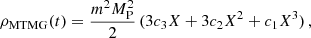
The second branch, called the normal branch, is the one which is considered in the present paper, and for which the following condition holds:

$$\begin{array}{c}\hfill H=\frac{\dot{a}}{\mathit{Na}}=X(t)\frac{\dot{\stackrel{\sim }{a}}}{M\stackrel{\sim }{a}}.\end{array}$$(15)

This leads in general to a time-dependent contribution in the Friedmann equation as follows

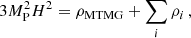$$\begin{array}{cc}\hfill 3M_{\mathrm{P}}^2{H}^2& ={\rho }_{\mathrm{MTMG}}+{\displaystyle \sum _i{\rho }_i,}\hfill \end{array}$$(16)

$$\begin{array}{cc}\hfill {\rho }_{\mathrm{MTMG}}(t)& =\frac{m^2{M}_{\mathrm{P}}^2}{2}(3c_{3}X+3c_2{X}^2+c_1{X}^3),\hfill \end{array}$$(17)

where ρ_i stands for any standard matter components (including possibly a pure cosmological constant). Therefore, there are interesting possibilities as the background can acquire non-trivial deviation from GR without introducing extra degrees of freedom.

The cosmological perturbation theory of MTMG has been studied in several papers (De Felice & Mukohyama 2017; Bolis et al. 2018), and we summarise in the following some results that will constitute the building blocks of our N-body study for MTMG.

First of all, while MTMG does not introduce any gravity degree of freedom besides the tensor modes, in the normal branch the dynamics of the matter degrees of freedom is indeed modified. In particular, if we study the dynamics of a cold and pressureless fluid, in the high-k regime, and fixing the dynamics of the background to be the same as in ΛCDM¹ for simplicity, we find that the energy density perturbation of the fluid satisfies the following equation of motion:

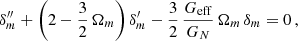$$\begin{array}{c}\hfill {\delta }_m^{″}+(2-\frac{3}{2}{\mathrm{\Omega }}_m){\delta }_m^{\prime }\frac{3}{2}\frac{G_{\mathrm{eff}}}{G_N}{\mathrm{\Omega }}_m{\delta }_m=0,\end{array}$$(18)

where

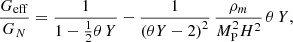$$\begin{array}{c}\hfill \frac{G_{\mathrm{eff}}}{G_N}=\frac{1}{1-\frac{1}{2}\theta Y}-\frac{1}{{(\theta Y-2)}^2}\frac{{\rho }_m}{M_{\mathrm{P}}^2{H}^2}\theta Y,\end{array}$$(19)

and θ is a free constant parameter defined as

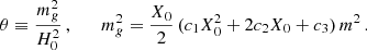$$\begin{array}{c}\hfill \theta \equiv \frac{m_g^2}{H_0^2},m_g^2=\frac{X_0}{2}(c_1{X}_0^2+2c_2{X}_0+c_3)m^2.\end{array}$$(20)

Furthermore, we have defined

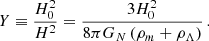$$\begin{array}{c}\hfill Y\equiv \frac{H_0^2}{H^2}=\frac{3H_0^2}{8\pi G_N({\rho }_m+{\rho }_{\mathrm{\Lambda }})}.\end{array}$$(21)

It should be noticed that whenever 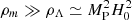${\rho }_m\gg {\rho }_{\Lambda }\simeq M_{\text{P}}^2{H}_0^2$, then θ Y → 0 (assuming θ to be of order unity), and G_eff/G_N → 1, which corresponds to the standard Newtonian limit. This limit in cosmology corresponds to the behaviour of the perturbations in the high-redshift limit.

In the following, for the N-body simulations, we consider the previous expression for G_eff to be valid locally at every point on the three-dimensional grid. This means that the variables Y and ρ_m are to be evaluated locally in the N-body simulation. This will automatically lead to the consequence that even today, in a overdense region, we would expect Y ≪ 1. In the following we find it convenient to introduce the following dimensionless quantities:

$$\begin{array}{c}\hfill {\eta }_{\mathrm{\Lambda }}\equiv \frac{{\rho }_{\mathrm{\Lambda }}}{{\overline{\rho }}_m}=\frac{{\mathrm{\Omega }}_{\mathrm{\Lambda }}\left(z\right)}{{\overline{\mathrm{\Omega }}}_m\left(z\right)}=\frac{1-{\overline{\mathrm{\Omega }}}_{m0}}{\frac{1}{a^3}{\overline{\mathrm{\Omega }}}_{m0}}=(\frac{1}{{\overline{\mathrm{\Omega }}}_{m0}}-1)a^3,\end{array}$$(22)

which is purely time-dependent; and

$$\begin{array}{c}\hfill {\eta }_m\equiv \frac{{\rho }_m}{{\overline{\rho }}_m},\end{array}$$(23)

so that, in overdense regions, one has η_m ≫ 1. Here, we consider all symbols with a bar to be evaluated on the FLRW background (or the volume average in the simulation). As a consequence, the average (background) matter density ${\overline{\rho }}_{\mathrm{m}}$ is

$$\begin{array}{c}\hfill {\overline{\rho }}_{\mathrm{m}}=\frac{3M_{\mathrm{P}}^2{H}_0^2{\overline{\mathrm{\Omega }}}_{m0}}{a^3},\end{array}$$(24)

leading to

$$\begin{array}{c}\hfill Y=\frac{a^3/{\overline{\mathrm{\Omega }}}_{m0}}{{\eta }_m+{\eta }_{\mathrm{\Lambda }}}.\end{array}$$(25)

Furthermore,

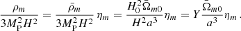$$\begin{array}{c}\hfill \frac{{\rho }_m}{3M_{\mathrm{P}}^2{H}^2}=\frac{{\overline{\rho }}_m}{3M_{\mathrm{P}}^2{H}^2}{\eta }_m=\frac{H_0^2{\overline{\mathrm{\Omega }}}_{m0}}{H^2{a}^3}{\eta }_m=Y\frac{{\overline{\mathrm{\Omega }}}_{m0}}{a^3}{\eta }_m.\end{array}$$(26)

To summarise, we implement the dynamics of the N-body simulations in RAMSES, taking into account the effective gravitational constant, G_eff, which is given locally by means of the following relation:

$$\begin{array}{c}\hfill \frac{G_{\mathrm{eff}}}{G_N}=\frac{1}{1-\frac{1}{2}\theta Y}-\frac{3{\overline{\mathrm{\Omega }}}_{m0}\theta Y^2{\eta }_m}{a^3{(\theta Y-2)}^2},\end{array}$$(27)

with Y being given by Eq. (25). Now we are ready to implement MTMG in our N-body simulations, so that we can start exploring the behaviour of gravity in MTMG in non-linear regimes.

3. Massive gravity implementation in RAMSES

To quantify the effects of MTMG in the cosmological evolution of structures, we run a set of cosmological simulations. The simulations are performed with a modified version of the N-body code RAMSES (Teyssier 2002).

The standard GR version of RAMSES solves Poisson’s equation ∇²Φ = 4πGδρ to find Φ at the centre of each grid cell. We note that $\delta \rho =\rho -\overline{\rho }$ can be either positive (for overdensities) or negative (for underdense regions). Solving the Poisson equation for a given distribution of matter gives us a continuous Φ field. One can then calculate the acceleration at the position of each particle as $\ddot{\mathbf{x}}=-\mathrm{\nabla }\mathrm{\Phi }$. The value of ∇Φ at the particle position is guessed by CIC linear interpolation from nearby grid cell centres (where the value is known). The particles are then moved one step in time using forward time integration with position, velocity, and acceleration.

In the case of MTMG, the Poisson equation is modified to ∇²Φ = 4πG_eff(ρ)δρ. One then needs to transform G → G_eff. This can be done either directly in the Poisson’s equation or when calculating the acceleration of each particle. We use the local G_eff in the Poisson equation when calculating the gravitational potential field. In this way, local gradients of the potential field, and hence the acceleration of matter, will be modified by structures elsewhere. This gives the correct long-range forces, where two clusters separated by a void feel the G_eff encoded in the void (see Sect. 4).

The initial matter distribution is generated with the package Grafic (Bertschinger 2001) with standard gravity. The approximation that we make without including modified gravity in the initial conditions is justified by the fact that modifications to GR occur only at much lower redshifts. All simulations use the same initial matter distribution and assume a flat ΛCDM background cosmology (see footnote 1 for MTMG in this respect) provided by the Planck collaboration: Ω_m = 0.3175, Ω_Λ = 0.6825, and H₀ = 67.11 km⁻¹ s⁻¹ Mpc⁻¹ (Planck Collaboration XVI 2014). The number of particles is 256³, and the size of the box is 64 Mpc h⁻¹.

4. Calibration of graviton mass

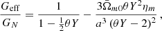
From a phenomenological viewpoint, one of the most important aspects of MTMG in the normal branch is that the effective gravitational constant G_eff depends on the environment. In linear perturbation theory, G_eff is a function of the energy density of the background FLRW universe and thus is homogeneous in space. As explained in the previous sections, in order to explore the non-linear dynamics of the normal branch of MTMG we promote G_eff to a function of a coarse-grained energy density so that it depends not only on the time but also on the spatial position and the coarse-graining scale. As G_eff is a non-linear function of the energy density, the spatial average of G_eff does not agree with G_eff for the averaged energy density, that is, 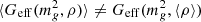$\langle G_{\text{eff}}(m_g^2,\rho )\rangle \ne G_{\text{eff}}(m_g^2,\langle \rho \rangle )$, where $m_g^2$ is the graviton mass squared, ρ is the energy density, ⟨X⟩ represents the volume average of a local function X. This makes it non-trivial to compare results from the non-linear simulation with predictions of the linear perturbation theory even at the largest scales.

To understand this point, suppose that there are two groups of particles separated from each other by a void region and that we would like to compute the gravitational force between a particle in one group and another particle in the other group. If the spatial size of each group is sufficiently small compared with the separation between the two groups then the strength of the gravitational force should be computed using the value of G_eff in the void region that separates the two groups. This means that the non-linear dynamics at largest scales should reflect the value of 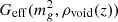$G_{\text{eff}}(m_g^2,{\rho }_{\text{void}}(z))$, where ρ_void(z) is the typical energy density in void regions at the redshift z. On the other hand, the predictions of the linear perturbation theory reflect the value of $G_{\text{eff}}(m_g^2,{\rho }_{\text{FLRW}}(z))$, where ρ_FLRW(z) = ⟨ρ_local(z, x)⟩ is the volume-averaged energy density, which corresponds to the FLRW background density at the redshift z. Here, ρ_local(z, x) is the local density at the redshift z and the spatial position x. In particular, the best-fit value of the graviton mass squared $m_g^2$ was obtained using 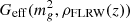$G_{\text{eff}}(m_g^2,{\rho }_{\text{FLRW}}(z))$. Therefore, provided that non-linear voids develop sufficiently at the redshift z = z_obs relevant for the observational bounds on $m_g^2$, we need to calibrate $m_g^2$ as $G_{\text{eff}}(m_{\text{nl}}^2,{\rho }_{\text{void}}(z_{\text{obs}}))=G_{\text{eff}}(m_{\text{lin}}^2,{\rho }_{\text{FLRW}}(z_{\text{obs}}))$, where $m_{\text{lin}}^2$ is the best-fit value of $m_g^2$ that was obtained using the prediction of the linear theory, and $m_{\text{nl}}^2$ is the calibrated graviton mass squared for the non-linear dynamics. In practice, we implement this idea of calibration as

$$\begin{array}{c}\hfill G_{\mathrm{eff},\mathrm{avg}}(m_{\mathrm{nl}}^2,z_{\mathrm{obs}})=G_{\mathrm{eff}}(m_{\mathrm{lin}}^2,{\rho }_{\mathrm{FLRW}}(z_{\mathrm{obs}})),\end{array}$$(28)

where

$$\begin{array}{c}\hfill G_{\mathrm{eff},\mathrm{avg}}(m_g^2,z)\equiv ⟨G_{\mathrm{eff}}(m_g^2,{\rho }_{\mathrm{local}}(z,\mathit{x}))⟩\end{array}$$(29)

is the volume-averaged effective gravitational constant. For $m_{\text{lin}}^2\simeq -3.828H_0^2$ obtained from the RSD data and the integrated Sachs-Wolfe-galaxy correlation data (De Felice & Mukohyama 2017; Bolis et al. 2018), z_obs ≃ 0 (to be more precise, z_obs ≃ 0−0.6 but we set z_obs ≃ 0 for simplicity) and $G_{\text{eff}}(m_{\text{lin}}^2,{\rho }_{\text{FLRW}}(z_{\text{obs}}))\simeq 0.45\times G_{\text{N}}$ (see Fig. 4 of De Felice & Mukohyama 2017), and thus

$$\begin{array}{c}\hfill m_{\mathrm{nl}}^2\simeq -1.7H_0^2.\end{array}$$(30)

Only after this calibration of the graviton mass can we make predictions by N-body simulations. Therefore, in the rest of the present paper, we adopt this value.

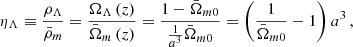
4.1. Average G_eff as a function of time

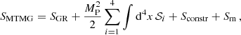
In Fig. 1 we plot the volume-averaged G_eff compared to the G_eff expected from the background ρ_m as a function of the scale factor. Here, we assume as an example θ = −1.7 because this is the calibrated best-fit value as explained in the previous paragraph. The necessity of the calibration, namely the difference between the volume-averaged G_eff and the G_eff for the averaged density, stems from the existence of voids where the density is lower than the average. At early times, voids have not yet developed and therefore the volume-averaged G_eff and the G_eff for the averaged density agree with each other. On the other hand, at late times, as voids develop, the volume-averaged G_eff begins to deviate from the G_eff for the averaged density. After a slight increase, the former starts to decrease significantly compared with the latter, as expected from Fig. 4 of De Felice & Mukohyama (2017), and as clearly seen in Fig. 1 of this paper. The 𝒪(1) difference between the two quantities at a = 1 clearly shows that the calibration is necessary to match predictions of the linear perturbation theory and those of non-linear N-body simulations.

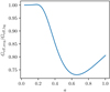Fig. 1. Volume averaged Geff compared to the Geff expected from the background ρm. The scale factor a is along the horizontal axis. Here, θ = −1.7. At early times when voids have not yet developed, effects of voids are negligible and therefore the averaged Geff and Geff for the average density agree with each other. On the other hand, at late times when voids are present, they deviate from each other due to the lower density in voids.

4.2. Void gravitational constant profile

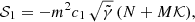
In Fig. 2 we plot the radial profile of G_eff around the centre of a deep void for θ = −1.7, θ = −3.828, and θ = 1.165. For negative θ, the effective gravitational constant, G_eff, is always smaller than G_N in low-density regions (such as voids). While for positive θ, the effective gravitational constant, G_eff, is larger than G_N in low-density regions. Models with a positive θ (resulting in increased G_eff in voids) are ruled out by the integrated Sachs-Wolfe-galaxy correlation data (Bolis et al. 2018) and are not be considered any further in this work.

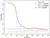Fig. 2. Profile of Geff around the centre of a deep void for θ = −1.7, θ = −3.828 and θ = 1.165. For negative values of θ, the effective gravitational constant, Geff, is always smaller than GN around voids.

5. Results

We performed three different simulations: GR (θ = 0), MTMG with θ = −3.828, and MTMG with θ = −1.7. For these choices of parameters, we ran high-resolution simulations with 1024³ particles and a box of 256 Mpc h⁻¹. Halos were calculated with the Rockstar halo finder (Behroozi et al. 2013).

5.1. Power spectra

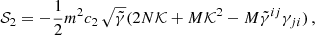
In Fig. 3 we plot the matter power spectrum for two different negative values of θ at redshift z = 0. The large-scale linear regime was studied in previous works (De Felice & Mukohyama 2017; Bolis et al. 2018) and the constraints obtained by the linear perturbation theory are valid as long as the graviton mass, or the parameter θ, is calibrated properly as explained in Sect. 4. For this reason, we focus on the non-linear small scales. From the figure, one can see that there is a suppression in the power spectra in the quasi-non-linear scales. As one enters the fully non-linear scales the power spectra approach GR, as we expect GR to be fully recovered at the very small-scale and high-density regions (in accordance with Fig. 4 of De Felice & Mukohyama 2017) when one approaches early times and high densities.

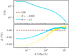Fig. 3. Small-scale power spectra at z = 0 for the high-resolution simulations. A suppression in the power spectra in the quasi-non-linear scales is present. As one enters the fully non-linear scales the power spectra approaches GR.

5.2. Halo mass function, mass histogram

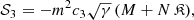
Figure 4 shows the halo mass function for MTMG. The lower panel shows the relative difference with respect to the same population in GR. One can see that MTMG creates a larger amount of massive halos in general, while there is a suppression of the abundance of small halos. This can be understood by taking into account the fact that smaller halos reside in relatively dense regions, where the effective gravitational constant can be larger than G_N, i.e. G_eff ≳ G_N (although G_eff → G_N in the high-density limit; see Fig. 6), and so the merger rate for substructures is higher than GR; small halos will interact to form larger halos at a higher rate.

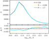Fig. 4. Halo mass function. Lower panel: relative difference with respect to the same population in GR. There are more massive halos in MTMG, while there is a suppression of the abundance of small halos.

5.3. Halo density profile

Figure 5 shows the dark matter density profile in a halo. The density is calculated as an average within concentric shells of some thickness Δr, centred on the coordinates of a given halo in the GR simulation. We expect similar halos to form at approximately the same coordinate in the other simulations because the initial particle distributions are identical. The halos have virial masses of 10¹⁴ − 10¹⁵ M_⊙ h⁻¹ and virial radii of about 2.0 Mpc h⁻¹. It is clear from this figure that the density profile is not a good probe for MTMG because the differences are small. We note that as one approaches the centre of the halo the density profile becomes similar to the GR one. This is expected as in this theory G_eff ∼ G_N in very high-density environments. On the other hand, at the outskirts of the halo, where the density of halos are lower and close to the critical density, G_eff < G_N and so the effects on the dark matter halo profiles differ from GR.

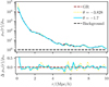Fig. 5. Dark matter halo density profile for GR and different negative θ. The black dashed line is the average background density. Lower panel: difference with respect to GR.

5.4. Halo gravitational constant profile

In Fig. 6 we show the effective gravitational constant G_eff, which is found by applying Eq. (27) to the density profiles around a halo. We see that G_eff tends towards G_N in the highest density regions, signifying a working screening. For intermediate densities in the outskirts of the halo (around 2−3 Mpc h⁻¹ or 1−2 r_vir from the centre), we see a slight enhancement of G_eff over G_N, which can lead to increased clustering at intermediate to small scales. As r further increases, G_eff/G_N tends to decrease and to have some oscillations. This behaviour is due to a decrement of the local environmental energy density (as moving out from the centre of the halo) and the peaks of the oscillations correspond to the presence of subhalos whose local density has some local peak.

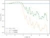Fig. 6. Profile of Geff around an isolated halo. Towards the centre of the halo, where the density is high, Geff approaches GN. On the other hand, in the outskirts of the halo Geff becomes smaller than GN. This effect is stronger for more negative values of θ.

5.5. Void density profile

Figure 7 shows the density profile of a void. The density is calculated as an average within concentric shells of some thickness Δr, centred on the coordinates of a given void in the GR simulation. We expect similar voids to form at approximately the same coordinate in the other simulations because the initial particle distributions are identical. A clear difference between MTMG and GR is that voids are denser near their centres in MTMG than in GR. This is because in MTMG, G_eff is lower than G_N in voids and so particles deep inside voids will not feel a force that attracts them to the boundaries of the voids (where the density is higher) as strongly as in GR.

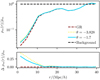Fig. 7. Density profile centred at a deep void. Voids are denser in MTMG than in GR, and their density profile depends on the value of θ.

6. Summary and discussion

We performed N-body simulations in the normal branch of the minimal theory of massive gravity (MTMG), employing the RAMSES code and implementing an environment-dependent effective gravitational constant G_eff as a function of the graviton mass and the local energy density as predicted in MTMG. We show how the effective gravitational coupling G_eff changes within voids and dark matter halos.

We find that halo density profiles are not a good probe for MTMG because deviations from GR are small. This is of no surprise because we expect MTMG to be screened, and to recover GR in high-density regions. Similarly, the matter power spectra show deviations only at the percentage level.

A clear difference between MTMG and GR is that voids are denser in MTMG than in GR. This is because in MTMG, G_eff is lower than G_N in voids, such that particles deep inside voids will not feel a strong force that attracts them to the structures outside of the voids (where the density is higher). As measuring voids profiles is currently a relatively complex task from an observational point of view, a better probe of MTMG would be the halo abundances. We find that MTMG creates a larger amount of massive halos, while there is a suppression of the abundance of small halos. This phenomenon is due to the fact that in overdense regions, in MTMG, we have G_eff ≳ G_N (and G_eff → G_N in very high-density regions). This leads, in general, to a stronger gravitational interaction among small subhalos in overdense regions, which in turn tends to build up a larger number of massive halos through mergers compared to GR.

The MTMG model with an environmentally dependent G_eff provides a framework rich in phenomenology. In this work, we find that MTMG has signatures distinguishable from GR on non-linear scales, while still being a good fit to current observations. Future observations and further studies of massive gravity in the non-linear regime will provide further insights into the nature of gravity.

Acknowledgments

RH and DFM thank the Research Council of Norway for their support. Computations were performed on resources provided by UNINETT Sigma2 – the National Infrastructure for High-Performance Computing and Data Storage in Norway. The work of ADF was supported by Japan Society for the Promotion of Science Grants-in-Aid for Scientific Research No. 20K03969. The work of SM was supported by Japan Society for the Promotion of Science Grants-in-Aid for Scientific Research No. 17H02890, No. 17H06359, and by World Premier International Research Center Initiative, MEXT, Japan.

References

All Figures

Fig. 1. Volume averaged Geff compared to the Geff expected from the background ρm. The scale factor a is along the horizontal axis. Here, θ = −1.7. At early times when voids have not yet developed, effects of voids are negligible and therefore the averaged Geff and Geff for the average density agree with each other. On the other hand, at late times when voids are present, they deviate from each other due to the lower density in voids.

In the text

	Fig. 2. Profile of Geff around the centre of a deep void for θ = −1.7, θ = −3.828 and θ = 1.165. For negative values of θ, the effective gravitational constant, Geff, is always smaller than GN around voids.
In the text

	Fig. 3. Small-scale power spectra at z = 0 for the high-resolution simulations. A suppression in the power spectra in the quasi-non-linear scales is present. As one enters the fully non-linear scales the power spectra approaches GR.
In the text

	Fig. 4. Halo mass function. Lower panel: relative difference with respect to the same population in GR. There are more massive halos in MTMG, while there is a suppression of the abundance of small halos.
In the text

	Fig. 5. Dark matter halo density profile for GR and different negative θ. The black dashed line is the average background density. Lower panel: difference with respect to GR.
In the text

	Fig. 6. Profile of Geff around an isolated halo. Towards the centre of the halo, where the density is high, Geff approaches GN. On the other hand, in the outskirts of the halo Geff becomes smaller than GN. This effect is stronger for more negative values of θ.
In the text

	Fig. 7. Density profile centred at a deep void. Voids are denser in MTMG than in GR, and their density profile depends on the value of θ.
In the text

References

- Aoki, K., Gorji, M. A., & Mukohyama, S. 2020, Phys. Lett. B, 810, 135843 [NASA ADS] [CrossRef] [Google Scholar]
- Behroozi, P. S., Wechsler, R. H., & Wu, H. Y. 2013, ApJ, 762, 109 [NASA ADS] [CrossRef] [Google Scholar]
- Bertschinger, E. 2001, ApJS, 137, 1 [NASA ADS] [CrossRef] [Google Scholar]
- Bolis, N., De Felice, A., & Mukohyama, S. 2018, Phys. Rev. D, 98, 024010 [NASA ADS] [CrossRef] [Google Scholar]
- Boulware, D., & Deser, S. 1972, Phys. Rev. D, 6, 3368 [CrossRef] [Google Scholar]
- D’Amico, G., de Rham, C., Dubovsky, S., et al. 2011, Phys. Rev. D, 84, 124046 [CrossRef] [Google Scholar]
- D’Amico, G., Gabadadze, G., Hui, L., & Pirtskhalava, D. 2013, Phys. Rev. D, 87, 064037 [Google Scholar]
- De Felice, A., & Mukohyama, S. 2016a, Phys. Lett. B, 752, 302 [NASA ADS] [CrossRef] [Google Scholar]
- De Felice, A., & Mukohyama, S. 2016b, JCAP, 04, 028 [CrossRef] [Google Scholar]
- De Felice, A., & Mukohyama, S. 2017, Phys. Rev. Lett., 118, 091104 [NASA ADS] [CrossRef] [Google Scholar]
- De Felice, A., Gumrukcuoglu, A., & Mukohyama, S. 2012, Phys. Rev. Lett., 109, 171101 [NASA ADS] [CrossRef] [Google Scholar]
- De Felice, A., Gumrukcuoglu, A., Lin, C., & Mukohyama, S. 2013, JCAP, 05, 035 [CrossRef] [Google Scholar]
- De Felice, A., Mukohyama, S., & Oliosi, M. 2017a, Phys. Rev. D, 96, 024032 [NASA ADS] [CrossRef] [Google Scholar]
- De Felice, A., Mukohyama, S., & Oliosi, M. 2017b, Phys. Rev. D, 96, 104036 [NASA ADS] [CrossRef] [Google Scholar]
- De Felice, A., Larrouturou, F., Mukohyama, S., & Oliosi, M. 2018, Phys. Rev. D, 98, 104031 [NASA ADS] [CrossRef] [Google Scholar]
- De Felice, A., Mukohyama, S., & Oliosi, M. 2019, Phys. Rev. D, 99, 044055 [CrossRef] [Google Scholar]
- De Felice, A., Doll, A., & Mukohyama, S. 2020, JCAP, 09, 034 [Google Scholar]
- de Rham, C., & Gabadadze, G. 2010, Phys. Rev. D, 82, 044020 [NASA ADS] [CrossRef] [Google Scholar]
- de Rham, C., Gabadadze, G., & Tolley, A. J. 2011, Phys. Rev. Lett., 106, 231101 [CrossRef] [Google Scholar]
- Fasiello, M., & Tolley, A. J. 2012, JCAP, 11, 035 [CrossRef] [Google Scholar]
- Fierz, M., & Pauli, W. 1939, Proc. R. Soc. Lond. A, A173, 211 [NASA ADS] [Google Scholar]
- Fujita, T., Kuroyanagi, S., Mizuno, S., & Mukohyama, S. 2019, Phys. Lett. B, 789, 215 [NASA ADS] [CrossRef] [Google Scholar]
- Fujita, T., Mizuno, S., & Mukohyama, S. 2020, JCAP, 01, 023 [Google Scholar]
- Gumrukcuoglu, A., Lin, C., & Mukohyama, S. 2011, JCAP, 11, 030 [CrossRef] [Google Scholar]
- Gumrukcuoglu, A., Lin, C., & Mukohyama, S. 2012, Phys. Lett. B, 717, 295 [NASA ADS] [CrossRef] [Google Scholar]
- Higuchi, A. 1987, Nucl. Phys. B, 282, 397 [CrossRef] [MathSciNet] [Google Scholar]
- Kenna-Allison, M., Gümrükçüoglu, A. E., & Koyama, K. 2020, Phys. Rev. D, 101, 084014 [CrossRef] [Google Scholar]
- Planck Collaboration XVI. 2014, A&A, 571, A16 [NASA ADS] [CrossRef] [EDP Sciences] [Google Scholar]
- Teyssier, R. 2002, A&A, 385, 337 [NASA ADS] [CrossRef] [EDP Sciences] [Google Scholar]
- Vainshtein, A. 1972, Phys. Lett. B, 39, 393 [Google Scholar]
- van Dam, H., & Veltman, M. 1970, Nucl. Phys. B, 22, 397 [CrossRef] [Google Scholar]
- Yao, Z. B., Oliosi, M., Gao, X., & Mukohyama, S. 2020, Phys. Rev. D, 103, 024032 [Google Scholar]
- Zakharov, V. 1970, JETP Lett., 12, 312 [Google Scholar]