| Issue |
A&A
Volume 652, August 2021
|
|
|---|---|---|
| Article Number | L2 | |
| Number of page(s) | 5 | |
| Section | Letters to the Editor | |
| DOI | https://doi.org/10.1051/0004-6361/202141395 | |
| Published online | 02 August 2021 | |
Letter to the Editor
A calibration of the Rossby number from asteroseismology
1
INAF – Osservatorio Astrofisico di Catania, Via S. Sofia, 78, 95123 Catania, Italy
e-mail: This email address is being protected from spambots. You need JavaScript enabled to view it.
2
Instituto de Astrofísica de Canarias, Santa Cruz de Tenerife, Spain
3
Department of Astrophysics, Universidad de La Laguna, Santa Cruz de Tenerife, Spain
4
AIM, CEA, CNRS, Université Paris-Saclay, Université Paris Diderot, Sorbonne Paris Cité, 91191 Gif-sur-Yvette, France
5
Department of Physics, University of Warwick, Coventry CV4 7AL, UK
6
Leibniz-Institut für Astrophysik Potsdam (AIP), An der Sternwarte 16, 14482 Potsdam, Germany
Received:
26
May
2021
Accepted:
15
July
2021
Abstract
Stellar activity and rotation are tightly related in a dynamo process. Our understanding of this mechanism is mainly limited by our capability of inferring the properties of stellar turbulent convection. In particular, the convective turnover time is a key ingredient through the estimation of the stellar Rossby number, which is the ratio of the rotation period and the convective turnover time. In this work, we propose a new calibration of the (B − V) color index dependence of the convective turnover time, hence, of the stellar Rossby number. Our new calibration is based on the stellar structure properties inferred through the detailed modeling of solar-like pulsators using asteroseismic observables. We show the impact of this calibration via a stellar activity-Rossby number diagram by applying it to a sample of about 40 000 stars observed with Kepler and for which the values for the photometric activity proxy Sph and surface rotation periods are available. Additionally, we provide a new calibration for the convective turnover time as function of the (GBP − GRP) color index for allowing applicability in the ESA Gaia photometric passbands.
Key words: stars: activity / starspots / stars: rotation / asteroseismology / convection / methods: statistical
© ESO 2021
1. Introduction
The study of the relationship between stellar activity and rotation represents one of the most important tests of stellar dynamo theory. In fact, while various types of dynamo action can be excited in solar-like stars (interface dynamo, α2Ω, or flux-transport dynamo, Brun & Browning 2017), the dependence of the α-effect taken from basic stellar parameters is not entirely unconstrained. In particular, for a turbulence with length scale ℓT, density ρ, and rotation Ω, it is possible to show that  , where D is the density length scale,
  , and vT is the convective velocity (Ruediger & Kichatinov 1993). This relation allows us to express the dynamo number Cα in terms of the rotation rate as Cα = Dα/η = 3τΩ, where η is the turbulent (eddies) diffusivity and τ is the convective turnover time. It is thus apparent that a larger value of τΩ (often called the Coriolis number) implies a lower threshold for the onset of the dynamo. However, while the rotation is, in principle, an observable quantity, τ generally depends on the efficiency of convection and, therefore, on the individual fundamental stellar parameters.
When interpreting observational data from low-mass stars, it is customary to weigh the relative importance of turbulent convection against rotation in terms of the stellar Rossby number as follows:
 (1)
(1)
where Prot is the surface rotation period, while τ is the convective turnover time, given as:
 (2)
(2)
with dCZ being the thickness of the convective envelope and  the average convective velocity (Brun et al. 2017).
In practice, τ is often determined from the semi-empirical (B − V) flux excess dependence obtained by Noyes et al. (1984), where a fixed value of the mixing-length parameter has been used. The limitation of this approach is already evident in the case of the Sun, where it yields τ ∼ 12 days, a value that is significantly smaller than the one obtained from a standard solar model, namely, ∼45 days (Bonanno et al. 2002).
If the turbulence is determined by only one length scale, it is not difficult to evaluate Eq. (2) from the fundamental stellar astrophysical parameters. In this case, if T is the temperature, cp the specific heat at constant pressure, and Hp the pressure scale height, the convective fluxes can be expressed as:
 (3)
(3)
where, in the last line, we assume ℓT/Hp ≈ 1.6, which is a typical value for a solar-like star. On the other hand, Fconv ≈ L/R2 and thus:
 (4)
(4)
With vs denoting the sound speed, we have
 (5)
(5)
where we make use of the fact that  . It is interesting to note that the estimation of Eq. (5) in Eq. (2) indeed represents a rather good estimate of the local convective turnover time at the base of the convection zone obtained from stellar models. In the case of the Sun, for instance, one obtains τ ≈ 45 days, a value that is consistent with the local value of (Hp/vT)r = 0.72 R⊙ for a fully calibrated solar standard model (Bonanno et al. 2002), which is in agreement with the calculation of Landin et al. (2010).
While the basic stellar parameters such as the luminosity, mass, and radius in Eq. (5) can easily be obtained at least for nearby stars, a reliable estimation of dCZ is generally a much more difficult task. Asteroseismology, however, can in principle provide us with this crucial piece of information for stars with well-characterized oscillation properties (e.g., see García & Ballot 2019). Similarly, by taking advantage of asteroseismic modeling, an estimation of the convective turnover time was carried out for ten stars by Mathur et al. (2014a). The authors computed the integral of the convective velocity over the convection zone but while using the profile of the convective velocity from the best-fit model obtained with seismic observables.
In this work, we thus propose to calibrate the empirical relation by Noyes et al. (1984) by exploiting a sample of main-sequence and sub-giant stars observed by the NASA Kepler mission (Borucki et al. 2010; Koch et al. 2010) and exhibiting solar-like oscillations. In particular, we seek to make use of this new calibration for a large sample of Kepler solar-like stars with known surface rotation periods, Prot, and photometric activity indexes, Sph. Brightness variations due to active regions co-rotating with the stellar surface provide constraints on both stellar properties (e.g., García et al. 2010; Reinhold et al. 2013; Nielsen et al. 2013; McQuillan et al. 2014; Mathur et al. 2014b; Salabert et al. 2016, 2017; Gordon et al. 2021). In this work, we show how the photometric activity index, Sph, is correlated with the Rossby number in a sample of ∼40 000 stars from Santos et al. (2019, 2021).
2. Observations and data
Our observational set comprises two samples of stars. The first sample consists of stars that have a detailed asteroseismic analysis available. This sample is used in Sect. 3 for obtaining a new calibration of the convective turnover time. The second sample contains stars that have a measure of their activity level and surface rotation. This sample is used in Sect. 4 to illustrate the implications of adopting our new calibration.
2.1. Calibration sample
To address the limitation of previous works aiming at obtaining a reliable estimate of the convective turnover time (e.g., Noyes et al. 1984; Lehtinen et al. 2021; See et al. 2021), we selected 62 G- and F-type stars from the Kepler LEGACY sample for which a precise determination of stellar parameters and chemical composition is available (Lund et al. 2017; Nissen et al. 2017; Silva Aguirre et al. 2017), along with BT, VT magnitudes from the Tycho-2 catalog (Høg et al. 2000). The LEGACY sample consists of the most well-characterized main-sequence and sub-giant stars observed by Kepler. Through the use of asteroseismology, the wealth of detailed oscillation mode properties measured in these stars allowed us to probe their internal structure with a high level of detail; in particular, hence, constraining the position of the base of the convection zone (CZ). This is essentially possible thanks to the probing power of individual mode frequencies, which are found in a large number for these stars thanks to the high-quality Kepler photometric observations, spanning more than three years in high duty-cycle. Stellar mass, radius, as well as the position of the base of the CZ, have been inferred with high precision, namely, about 2% in radius and 4% in mass. As already described in Sect. 1, these are key quantities that are needed to define the convective turnover time in these stars.
2.2. Stellar activity sample
The long-term continuous observations collected by Kepler are suitable for constraining stellar magnetic activity and rotation. Recently, the sample of known rotation periods, Prot, and photometric activity proxies, Sph, was greatly extended thanks to the use of KEPSEISMIC1 light curves (García et al. 2011, 2014a; Pires et al. 2015) of mid-F to M stars observed by Kepler, (Santos et al. 2019, 2021). Indeed, more than 60% of new Prot detections were reported, compared to the previous largest rotation-period catalog (McQuillan et al. 2014). The rotation-period candidates were obtained by combining the wavelet analysis and the autocorrelation function of the light curves (Mathur et al. 2010; García et al. 2014b; Ceillier et al. 2016, 2017), while the reliable rotation periods were selected through a machine-learning algorithm (ROOSTER; Breton et al. 2021), automatic selection, and visual inspection (Santos et al. 2019, 2021). Having Prot, we can then compute Sph as the standard deviation over light curve segments of length 5 × Prot (Mathur et al. 2014a). Salabert et al. (2016, 2017) have shown that Sph is an appropriate proxy for stellar magnetic activity.
Starting with a sample of 55 232 stars from Santos et al. (2019, 2021), and Mathur et al. (in prep.), which inclues F, G, K, and M dwarfs, as well as subgiants, we first removed the subgiants by making a crude cut on the surface gravity, taking only stars with log g above 4.2 dex. We then collected the B and V magnitudes from the American Association of Variable Star Observers Photometric All-Sky Survey (Henden et al. 2015)2. We further discarded stars flagged as close-in binary candidates by Santos et al. (2019, 2021), which led us to a sample of 39 125 stars with inferred Prot and Sph.
3. Bayesian inference
Following from Eqs. (2) and (5), τc can be expressed in terms of fundamental stellar properties as:
 (6)
(6)
where in the case of the LEGACY sample the quantities R, RCZ, L, M are obtained from the stellar and asteroseismic modeling performed by Silva Aguirre et al. (2017)3 using the ASTFIT pipeline, a combination of ASTEC (Aarhus STellar Evolution Code) for stellar evolutionary models (Christensen-Dalsgaard 2008a) and ADIPLS (Aarhus adiabatic oscillation package) for theoretical pulsation frequencies (Christensen-Dalsgaard 2008b). We therefore compare the outcome of Eq. (6), hereafter τc, LEGACY, to that obtained from the original semi-empirical relation presented by Noyes et al. (1984), namely:
 (7)
(7)
where x = 1 − (B − V), which we refer to as τc, N84 for clarity. We note that the relation presented by Noyes et al. (1984) has to be evaluated by means of the Johnson-Cousin B and V magnitudes, which differ from those available for the LEGACY sample, corresponding to Tycho catalog BT and VT magnitudes. For the purpose of obtaining a proper comparison between the two convective turnover times considered here, we therefore applied a transformation converting our Tycho (BT − VT) color index into a (B − V) one following ESA97 Vol. 1, Sect. 1.3.
3.1. Calibration with B–V color
Our basic assumption is that a relation between τc, LEGACY and (B − V) color could be represented by a linear law of the type
 (8)
(8)
However, we also incorporate the possibility of having departures from a simple linear relation. We therefore consider an additional law involving a quadratic dependence on (B − V) of the type:
 (9)
(9)
For the purpose of obtaining the estimates of the free parameters (a1, a2) of Eq. (8) and (b1, b2, b3) of Eq. (9), we made use of a Bayesian parameter estimation. This procedure is carried out by means of the public tool DIAMONDS4 (high-DImensional And multi-MOdal NesteD Sampling, Corsaro & De Ridder 2014), based on the nested sampling Monte Carlo algorithm (Skilling 2004). Here, we adopt a standard Normal likelihood function, assuming a conservative theoretical uncertainty of one day on each estimate of τc,LEGACY, along with uniform priors on all free parameters.
To test the significance of having a quadratic dependence between τc,LEGACY and (B − V), we performed a Bayesian model comparison by means of the Bayesian evidence computed by DIAMONDS. In this case, we compare the model obtained using Eq. (8) with the one of Eq. (9). We find that the corresponding Bayes’ factor ℬquadratic, linear ≃ 95 significantly exceeds the condition for a strong evidence (Jeffreys 1961), strongly thus favoring the scenario of a quadratic dependence. This implies that the adoption of Eq. (9) is by far statistically justified when adopting the LEGACY sample as a calibration set. The result of this inference process is presented in Fig. 1 (left panel), where the quadratic trend appears dominant along the entire range investigated, that is, (0.38 < (B − V) < 0.75, corresponding to 1 ≲ τc, N84 ≲ 17 days), with the coefficients  d,
d,  d mag−1, and
  d mag−2. We further point out that this relation intrinsically incorporates the effect of a varying metallicity from star to star because the stellar properties used for the evaluation of the convective turnover time are the product of a detailed asteroseismic and stellar structure modeling that also take the metallicity into account. This can be seen in Fig. 1, where the color-coding of the symbols indicating the metallicities adopted by Lund et al. (2017) shows no evidence of a preferential trend with τc, LEGACY.
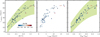 |
Fig. 1. Convective turnover time for the LEGACY sample, τc, LEGACY. Left panel: quadratic fit using Eq. (9) as a function of (B − V) color as a solid black line, with the green shaded area representing the 1-σ credible region obtained from the Bayesian inference. The color coding shows the stellar metallicity reported by Lund et al. (2017). Right panel: details are similar to those of the left panel, but showing the result as a function of the Gaia (GBP − GRP) color, with the quadratic fit from Eq. (11) overlaid. Middle panel: comparison between τc, LEGACY and τc, N84 as obtained by means of the (B − V) color. |
3.2. Calibration with Gaia GBP–GRP color
We adopted new Gaia EDR3 (GBP − GRP)-pagination colors (Gaia Collaboration 2021) for studying the following relation: τc,LEGACY–(GBP − GRP). This relation is of particular usefulness and applicability for obtaining a reliable estimation of the stellar convective turnover time in the context of the very large catalog parameters available from ESA Gaia.
Following the approach presented for the calibration of a τc,LEGACY–(B − V) relation, we performed a Bayesian parameter estimation for both a linear and a quadratic model of the type:
 (10)
(10)
and
 (11)
(11)
Similarly to what was obtained for the Johnson-Cousin photometric system, our Bayesian model comparison process (resulting from a Bayes’ factor ln ℬlinear, quadratic ≃ 101) indicates that a quadratic model is strongly favored for interpreting the observed trend when using Gaia colors in the range of 0.55 < (GBP − GRP) < 0.97. This trend is already evident from Fig. 1 (right panel). The estimated parameters of the quadratic model are  d,
d,  d mag−1, and
  d mag−2.
4. Results
Our Eq. (9), by means of a direct dependence from the (B − V) color index, allows us to estimate a proper turbulent time-scale for a dynamo action deeply seated at the bottom of the CZ, at least for stars close to the main sequence. The estimated convective turnover time for the LEGACY sample appears to be strongly correlated to that obtained from the standard relation by Noyes et al. (1984), although this dependence is clearly not linear (Fig. 2, middle panel). In addition, we extended the applicability of this kind of dependence to the Gaia photometric system by calibrating another relation that can be used to obtain a convective turnover time directly from the (GBP − GRP) color index.
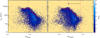 |
Fig. 2. Stellar activity index Sph as a function of the Rossby number. Left panel: Rossby number evaluated with the semi-empirical relation by Noyes et al. (1984). Right panel: details are similar to the left panel, but using the Rossby number evaluated with the new convective turnover time from Eq. (9). The thick red lines represent the maximum Sph of the 95 percentile of each chunk in Rossby number, evaluated in a range centered around the kink. Sun symbols mark the position of the Sun between the minimum and maximum of activity (RoNoyes, ⊙ = 1.989, RoLEGACY, ⊙ = 0.496). The position of the kink is marked by the vertical dashed and dot-dashed lines, for the left and right panel, respectively. The left-pointing arrow shows how the position of the kink shifts when switching from τc, N84 to τc, LEGACY. The density of stars is indicated by the blue color scale. |
To illustrate the implications of our new calibration, we have applied it in comparison to the standard Noyes’ formulation (Noyes et al. 1984) for a large sample of stars observed by Kepler with measured rotation periods and presented in Sect. 2.2. We show the result in Fig. 2, where the photometric activity index Sph is plotted as a function of the Rossby number, evaluated using both the Noyes’ prescription (left panel of Fig. 2) and our new calibration (right panel of Fig. 2) for stars having (B − V) within the range provided for our new calibration (see Sect. 3, 16 844 targets in total). For highlighting the presence of a kink in the distribution, we binned the sample into 50 chunks, having constant size in a logarithm of the Rossby number. For each chunk, we computed the maximum out of the lowest 95 percentile in Sph of the corresponding portion of the star sample. The outcome is shown as a thick red line, which clearly follows the shape of the top edge of the distribution. Here, it can be seen that the kink corresponding to the change in regime from saturation to a linear dependence of the photometric activity index as a function of the Rossby number shifts from Ro ∼ 0.82 when using the Noyes’ prescription (Noyes et al. 1984) to Ro ∼ 0.23 when adopting our newly calibrated τc from Eq. (9). The extent of the shift of the kink position in Rossby number (e.g., See et al. 2021) is emphasized by the left-pointing arrow in the right panel of Fig. 2. The position of the Sun is also shown, with Sph computed at the minimum and maximum of activity (Mathur et al. 2019). It is reassuring that our result based on the adoption of τc, LEGACY appears to be in agreement with the findings by See et al. (2021). In their work, the authors adopted the photometric variability amplitude, Rper, originally introduced by Basri et al. (2010), and a Rossby number obtained from model structure grids and rotation periods from McQuillan et al. (2014).
Finally, we point out that care is needed when dealing with more massive F-type stars (M ≳ 1.3 M⊙). Because of their thin convective envelopes, these stars happen to fall at the lower edge of the range of convective turnover times covered by our calibration set (say τN84 < 3 days). This implies that the derived quadratic law from Eq. (9), when adopting (B − V), and from Eq. (11) for the (GBP − GRP) colors, may be less accurate in this regime. Future improvements of the proposed relation will aim at including additional stars in this region of small convective turnover time within the calibration sample.
5. Conclusions
The estimation of a proper convective turnover time is essential for our comprehension of the stellar dynamo action through the Rossby number. In this work, we have shown that starting from the observed color of the star, and specifically the (B − V) color index from the Johnson-Cousin photometric system and the (GBP − GRP) color index from ESA Gaia, it is possible to obtain a reliable estimate of a local convective turnover time that is comparable to the one obtained by stellar models and evaluated at the bottom of the CZ. In particular, we note that through the adoption of Eq. (6) it is possible to evaluate a proper convective turnover time for large samples of stars without the need of computing stellar models. This is supported by the agreement found in the location of the kink of the relation between our photometric stellar activity index, Sph, and the Rossby number (see Fig. 2), and the one presented by See et al. (2021), where the computation of the convective turnover time is instead based on the adoption of stellar model grids.
We find that these new calibrations pave the way for future studies of the dynamo theory that are based on the adoption of photometric activity indices obtained from past and ongoing space missions such as NASA Kepler, K2 (Howell et al. 2014), the NASA Transiting Exoplanet Survey Satellite (TESS; Ricker et al. 2014), as well as the upcoming ESA PLanetary Transits and Oscillations of stars (PLATO; Rauer et al. 2014). This result opens up the possibility to perform detailed statistical studies that can be extended to very large stellar populations spanning a wide range of fundamental properties and rotation. This is of particular relevance in the context of the vast amount of color information being provided by ESA Gaia space mission. Future improvements on the stellar modeling through the inclusion of internal dynamical processes, for instance, angular momentum transport, could be exploited to further refine our knowledge of these relationships.
Acknowledgments
We thank the referee Dr. Travis Metcalfe for valuable comments that helped in improving the manuscript. E.C. and A.B. acknowledge support from PLATO ASI-INAF agreement no. 2015-019-R.1-2018. S.M. acknowledges support by the Spanish Ministry of Science and Innovation with the Ramon y Cajal fellowship number RYC-2015-17697 and the grant number PID2019-107187GB-I00. R.A.G. and S.N.B. acknowledge the support from the CNES GOLF and PLATO grants. A.R.G.S. acknowledges the support of the STFC consolidated grant ST/T000252/1 and NASA grant No. NNX17AF27.
References
- Basri, G., Walkowicz, L. M., Batalha, N., et al. 2010, ApJ, 713, L155 [Google Scholar]
- Bonanno, A., Schlattl, H., & Paternò, L. 2002, A&A, 390, 1115 [NASA ADS] [CrossRef] [EDP Sciences] [MathSciNet] [Google Scholar]
- Borucki, W. J., Koch, D., Basri, G., et al. 2010, Science, 327, 977 [NASA ADS] [CrossRef] [PubMed] [Google Scholar]
- Breton, S. N., Santos, A. R. G., Bugnet, L., et al. 2021, A&A, 647, A125 [EDP Sciences] [Google Scholar]
- Brun, A. S., & Browning, M. K. 2017, Liv. Rev. Sol. Phys., 14, 4 [Google Scholar]
- Brun, A. S., Strugarek, A., Varela, J., et al. 2017, ApJ, 836, 192 [NASA ADS] [CrossRef] [Google Scholar]
- Ceillier, T., van Saders, J., García, R. A., et al. 2016, MNRAS, 456, 119 [NASA ADS] [CrossRef] [Google Scholar]
- Ceillier, T., Tayar, J., Mathur, S., et al. 2017, A&A, 605, A111 [NASA ADS] [CrossRef] [EDP Sciences] [Google Scholar]
- Christensen-Dalsgaard, J. 2008a, Ap&SS, 316, 13 [NASA ADS] [CrossRef] [Google Scholar]
- Christensen-Dalsgaard, J. 2008b, Ap&SS, 316, 113 [Google Scholar]
- Corsaro, E., & De Ridder, J. 2014, A&A, 571, A71 [NASA ADS] [CrossRef] [EDP Sciences] [Google Scholar]
- Gaia Collaboration (Brown, A. G. A., et al.) 2021, A&A, 649, A1 [NASA ADS] [CrossRef] [EDP Sciences] [Google Scholar]
- García, R. A., & Ballot, J. 2019, Liv. Rev. Sol. Phys., 16, 4 [Google Scholar]
- García, R. A., Mathur, S., Salabert, D., et al. 2010, Science, 329, 1032 [Google Scholar]
- García, R. A., Hekker, S., Stello, D., et al. 2011, MNRAS, 414, L6 [NASA ADS] [CrossRef] [Google Scholar]
- García, R. A., Mathur, S., Pires, S., et al. 2014a, A&A, 568, A10 [NASA ADS] [CrossRef] [EDP Sciences] [Google Scholar]
- García, R. A., Ceillier, T., Salabert, D., et al. 2014b, A&A, 572, A34 [NASA ADS] [CrossRef] [EDP Sciences] [Google Scholar]
- Gordon, T. A., Davenport, J. R. A., Angus, R., et al. 2021, ApJ, 913, 70 [Google Scholar]
- Henden, A. A., Levine, S., Terrell, D., & Welch, D. L. 2015, Am. Astron. Soc. Meet. Abstr., 225, 336.16 [Google Scholar]
- Høg, E., Fabricius, C., Makarov, V. V., et al. 2000, A&A, 355, L27 [Google Scholar]
- Howell, S. B., Sobeck, C., Haas, M., et al. 2014, PASP, 126, 398 [NASA ADS] [CrossRef] [Google Scholar]
- Jeffreys, H. 1961, Theory of Probability, 3rd edn. (Oxford: Oxford University Press) [Google Scholar]
- Koch, D. G., Borucki, W. J., Basri, G., et al. 2010, ApJ, 713, L79 [NASA ADS] [CrossRef] [Google Scholar]
- Landin, N. R., Mendes, L. T. S., & Vaz, L. P. R. 2010, A&A, 510, A46 [NASA ADS] [CrossRef] [EDP Sciences] [Google Scholar]
- Lehtinen, J. J., Käpylä, M. J., Olspert, N., & Spada, F. 2021, ApJ, 910, 110 [Google Scholar]
- Lund, M. N., Silva Aguirre, V., Davies, G. R., et al. 2017, ApJ, 835, 172 [Google Scholar]
- Mathur, S., García, R. A., Régulo, C., et al. 2010, A&A, 511, A46 [NASA ADS] [CrossRef] [EDP Sciences] [Google Scholar]
- Mathur, S., García, R. A., Ballot, J., et al. 2014a, A&A, 562, A124 [NASA ADS] [CrossRef] [EDP Sciences] [Google Scholar]
- Mathur, S., Salabert, D., García, R. A., & Ceillier, T. 2014b, J. Space Weather Space Clim., 4, A15 [NASA ADS] [CrossRef] [EDP Sciences] [MathSciNet] [Google Scholar]
- Mathur, S., García, R. A., Bugnet, L., et al. 2019, Front. Astron. Space Sci., 6, 46 [CrossRef] [Google Scholar]
- McQuillan, A., Mazeh, T., & Aigrain, S. 2014, ApJS, 211, 24 [NASA ADS] [CrossRef] [MathSciNet] [Google Scholar]
- Nielsen, M. B., Gizon, L., Schunker, H., & Karoff, C. 2013, A&A, 557, L10 [NASA ADS] [CrossRef] [EDP Sciences] [Google Scholar]
- Nissen, P. E., Silva Aguirre, V., Christensen-Dalsgaard, J., et al. 2017, A&A, 608, A112 [NASA ADS] [CrossRef] [EDP Sciences] [Google Scholar]
- Noyes, R. W., Hartmann, L. W., Baliunas, S. L., Duncan, D. K., & Vaughan, A. H. 1984, ApJ, 279, 763 [NASA ADS] [CrossRef] [Google Scholar]
- Pires, S., Mathur, S., García, R. A., et al. 2015, A&A, 574, A18 [NASA ADS] [CrossRef] [EDP Sciences] [Google Scholar]
- Rauer, H., Catala, C., Aerts, C., et al. 2014, Exp. Astron., 38, 249 [Google Scholar]
- Reinhold, T., Reiners, A., & Basri, G. 2013, A&A, 560, A4 [NASA ADS] [CrossRef] [EDP Sciences] [Google Scholar]
- Ricker, G. R., Winn, J. N., Vanderspek, R., et al. 2014, SPIE Conf. Ser., 9143, 20 [Google Scholar]
- Ruediger, G., & Kichatinov, L. L. 1993, A&A, 269, 581 [NASA ADS] [Google Scholar]
- Salabert, D., García, R. A., Beck, P. G., et al. 2016, A&A, 596, A31 [NASA ADS] [CrossRef] [EDP Sciences] [Google Scholar]
- Salabert, D., García, R. A., Jiménez, A., et al. 2017, A&A, 608, A87 [NASA ADS] [CrossRef] [EDP Sciences] [Google Scholar]
- Santos, A. R. G., García, R. A., Mathur, S., et al. 2019, ApJS, 244, 21 [Google Scholar]
- Santos, A. R. G., Breton, S. N., Mathur, S., & García, R. A. 2021, ApJS, submitted [arXiv:2107.02217] [Google Scholar]
- See, V., Roquette, J., Amard, L., & Matt, S. P. 2021, ApJ, 912, 127 [Google Scholar]
- Silva Aguirre, V., Lund, M. N., Antia, H. M., et al. 2017, ApJ, 835, 173 [Google Scholar]
- Skilling, J. 2004, AIP Conf. Proc., 735, 395 [Google Scholar]
All Figures
|
Fig. 1. Convective turnover time for the LEGACY sample, τc, LEGACY. Left panel: quadratic fit using Eq. (9) as a function of (B − V) color as a solid black line, with the green shaded area representing the 1-σ credible region obtained from the Bayesian inference. The color coding shows the stellar metallicity reported by Lund et al. (2017). Right panel: details are similar to those of the left panel, but showing the result as a function of the Gaia (GBP − GRP) color, with the quadratic fit from Eq. (11) overlaid. Middle panel: comparison between τc, LEGACY and τc, N84 as obtained by means of the (B − V) color. |
| In the text | |
|
Fig. 2. Stellar activity index Sph as a function of the Rossby number. Left panel: Rossby number evaluated with the semi-empirical relation by Noyes et al. (1984). Right panel: details are similar to the left panel, but using the Rossby number evaluated with the new convective turnover time from Eq. (9). The thick red lines represent the maximum Sph of the 95 percentile of each chunk in Rossby number, evaluated in a range centered around the kink. Sun symbols mark the position of the Sun between the minimum and maximum of activity (RoNoyes, ⊙ = 1.989, RoLEGACY, ⊙ = 0.496). The position of the kink is marked by the vertical dashed and dot-dashed lines, for the left and right panel, respectively. The left-pointing arrow shows how the position of the kink shifts when switching from τc, N84 to τc, LEGACY. The density of stars is indicated by the blue color scale. |
| In the text | |
Current usage metrics show cumulative count of Article Views (full-text article views including HTML views, PDF and ePub downloads, according to the available data) and Abstracts Views on Vision4Press platform.
Data correspond to usage on the plateform after 2015. The current usage metrics is available 48-96 hours after online publication and is updated daily on week days.
Initial download of the metrics may take a while.