| Issue |
A&A
Volume 652, August 2021
|
|
|---|---|---|
| Article Number | A8 | |
| Number of page(s) | 7 | |
| Section | Extragalactic astronomy | |
| DOI | https://doi.org/10.1051/0004-6361/202141040 | |
| Published online | 30 July 2021 | |
Gravitational collapse from cold uniform asymmetric initial conditions
1
Centro Ricerche Enrico Fermi, Via Panisperna 89 A, 00184 Rome, Italy
e-mail: This email address is being protected from spambots. You need JavaScript enabled to view it.
2
Istituto Nazionale Fisica Nucleare, Unità Roma 1, Dipartimento di Fisica, Università di Roma “Sapienza”, Piazzale Aldo Moro 2, 00185 Roma, Italy
3
Laboratoire de Physique Nucléaire et de Hautes Énergies, UPMC IN2P3 CNRS UMR 7585, Sorbonne Université, 4 place Jussieu, 75252 Paris Cedex 05, France
Received:
9
April
2021
Accepted:
25
May
2021
Abstract
Using controlled numerical N-body experiments, we show how, in the collapse dynamics of an initially cold and uniform distribution of particles with a generic asymmetric shape, finite N fluctuations and perturbations induced by the anisotropic gravitational field compete to determine the physical properties of the asymptotic quasi-stationary state. When finite N fluctuations dominate the dynamics, the particle energy distribution changes greatly and the final density profile decays outside its core as r−4 with an N-dependent amplitude. On the other hand, in the limit where the anisotropic perturbations dominate, the collapse is softer and the density profile shows a decay as r−3, as is typical of halos in cosmological simulations. However, even in this limit, convergence with N of the macroscopic properties of the virialized system, such as the particle energy distributions, the bound mass, and the density profile, is very slow and not clearly established, including for our largest simulations (with N ∼ 106). Our results illustrate the challenges of accurately simulating the first collapsing structures in standard-type cosmological models.
Key words: methods: numerical / galaxies: formation / galaxies: elliptical and lenticular, cD
© ESO 2021
1. Introduction
The evolution under Newtonian self-gravity of an isolated distribution of particles that start from initial conditions (ICs) in which the particles are initially at rest and are randomly distributed in a sphere with uniform mean density has been studied by numerous authors since the earliest numerical simulations of such systems. Numerous variants have also been explored, notably with initial velocity dispersion using radially dependent density profiles and for spheroidal boundaries (Henon 1964, 1973; van Albada 1982; Merritt & Aguilar 1985; Aarseth et al. 1988; Aguilar & Merritt 1990; Theis & Spurzem 1999; Boily et al. 2002; Roy & Perez 2004; Boily & Athanassoula 2006; Barnes et al. 2009; Joyce et al. 2009; Sylos Labini 2012, 2013; Worrakitpoonpon 2015, 2020; Sylos Labini et al. 2015, 2020; Benhaiem & Sylos Labini 2015, 2017; Benhaiem et al. 2016; Spera & Capuzzo-Dolcetta 2017). Such systems provide a natural and simple setting to explore the rich complexity of the nonlinear phase of gravitational dynamics relevant to many different problems in astrophysics and cosmology. Though in the context of structure formation in cosmology structures are never strictly isolated, these simple models are nonetheless highly relevant. Indeed, the so-called spherical collapse model, which analytically describes a smooth spherical over-density in an expanding universe, is a paradigmatic model that guides understanding of nonlinear cosmological structure formation (see, e.g., Peebles 1980). Despite its simplicity, and indeed its breakdown in a singularity at a finite time, it describes qualitatively well what is actually observed in N-body simulations of standard cosmological models: Over-dense regions expand more slowly on average until they “break off” from the expansion and undergo a strong collapse, starting from conditions that are effectively those of an isolated, initially cold configuration. The specific design of any set of numerical experiments in either the astrophysical or cosmological context varies depending on the motivation of the authors and the physical issues they focus on. We report here a study of a very simple variant of this class of models. It is designed to explore how deviations from spherical symmetry compete with the density fluctuations intrinsic to the discrete particle distribution in regulating the singularity in the limit of a cold uniform collapse (i.e., of the spherical collapse model in cosmology). The understanding of the dynamics that can result from the very simple class of ICs we consider – with just one parameter in addition to the particle number – is of broad interest. More specifically, as we explain, it gives insight into the challenges of accurately simulating the first nonlinear structures in many cosmological models.
One particular question that can be addressed in a controlled manner with these systems is the extent to which the evolution of discrete N-body systems approximate, and converge to, in an appropriate N → ∞ limit, the continuum limit given by the Vlasov-Poisson system (or collisionless Boltzmann equations) for a smooth phase-space density. Indeed, for the relevant physical problems, the particles of the N-body simulations are usually thought of not as physical particles but simply as a tool for representing the physical phase-space density, the evolution of which is described by these equations. In the cosmological context the physical particles are usually microscopic dark matter particles, while the particles of simulations are unphysical “macro-particles” with astrophysical-scale masses. An important question is then to what extent the results obtained from these simulations are dependent on N and what the associated limit on their accuracy is. In more physical terms the question can be formulated as to what extent the fluctuations associated with the particle discretization play a role in the dynamics in its nonlinear phase. This question of N-body discretization effects in cosmology can be straightforwardly addressed using isolated systems because, as noted, we can consider, in light of the exact spherical collapse model, that nonlinear structure formation can be approximated by the collapse of quasi-isolated initially cold clumps.
In current models of cosmological structure formation, there is always a minimal scale in the initial spectrum of fluctuations, the physical size of which varies greatly depending on whether the supposed dark matter is “cold” or “warm” (see, e.g., Wang & White 2007; Kuhlen et al. 2012, and references therein). The first clumps therefore form starting from fluctuations at this scale and are initially highly uniform at smaller scales. In the discretized version of the problem (i.e., as represented in an N-body simulation) there are, in addition, the fluctuations associated with the particle discretization. The question of discreteness effects thus appears to be well and simply posed in terms of the N dependence of the evolution of an isolated, initially cold, uniform clump. However, things are not so simple because, in spherical symmetry, the N → ∞ limit has the finite time collapse singularity of the spherical collapse model. Spheroidal clumps are a simple alternative, but they are also characterized by a singularity in the same limit due to their residual rotational symmetry (Lin et al. 1965; Worrakitpoonpon 2020).
In a recent article, Sylos Labini & Capuzzo-Dolcetta (2020) considered ICs that are spherical but with a simple family of density fluctuations within the sphere of which the amplitude is regulated by a single additional parameter. This reproduces ICs that are expected to model clumps forming from preexisting structures at smaller scales, as at later times in typical cosmological models. Here we instead consider modeling the clumps as being uniform at small scales but having an irregular shape. This is a good schematic representation of the first collapsing structures in a standard cosmological model.
The cold uniform spherical case, with a single free parameter, N, has been studied at length in, for example, Aarseth et al. (1988) and Joyce et al. (2009). In this case the singularity in the N → ∞ is thus regularized by the density fluctuations associated with discreteness alone. More specifically, it is found, for Poisson-distributed particles, that the minimal system radius approximately scales as rmin ∼ N−1/3. This behavior can be derived from the growth of the density perturbations in the bulk, which evolve until the associated peculiar kinetic energy becomes on the order of the gravitational potential energy. Thus, the smaller N is (i.e., the larger the initial density fluctuations), the softer the collapse is: As a consequence of the larger resulting particle peculiar velocities, the collapse phase stops earlier. In addition, the properties of the virialized quasi-stationary state (QSS; e.g., the amplitude of the density profile and the particle energy distribution) that is attained rapidly after the collapse are N dependent. In the model considered by Sylos Labini & Capuzzo-Dolcetta (2020), the particles are instead distributed in Nc spherical sub-clumps of radius r; r is smaller than the radius of the system itself, R, which allows the amplitude of initial fluctuations to be regulated. As their amplitude is increased, the very violent collapse of the simple model is progressively “softened”: While in the former case there is a large change in the particle energy distribution driven by a strong variation in the system’s mean field, in the latter there is a marginal change in the system’s phase-space distribution. The properties of the QSS reached thus depend strongly on whether the collapse was violent or soft: In particular, the final density profile decreases as ∼r−4 when it is very violent, while it decreases as ∼r−3 in the soft limit. In the model we explore here, we again see these same limiting behaviors emerge.
The term “violent relaxation” that we employ here was introduced by Lynden-Bell (1967) to describe the collective mean-field relaxation process that drives a self-gravitating system prepared in an out-of-equilibrium IC to form a QSS. Lynden-Bell also proposed a theory to calculate the resulting QSS using a statistical approach based on the collisionless Boltzmann equation. The predictions of this theory have, however, been shown by the results of numerical experiments (see, e.g., Arad & Lynden-Bell 2005) to not account well for the relaxed QSS of such systems. We note that, for the ICs we study here, the theory of Lynden-Bell cannot be adequate for a very simple reason: It assumes the mass and energy of the QSS to be that of the initial state, while these systems are always characterized – because of the violence of the relaxation – by the ejection of a very significant fraction of their initial mass and energy. We note that a very different semi-analytic model of violent relaxation that does admit the presence of ejected mass has been proposed by Mangalam et al. (1999). It is based on the physical picture of strong and short-lived interactions between the system’s potential fluctuations and particle orbits and, interestingly, also accounts for an associated QSS density profile decreasing as ∼r−4.
In this work we introduce and use numerical experiments to study a simple toy model in which the perturbations of shape and the finite N fluctuations can be varied independently by tuning two parameters: a “shape parameter,” p, which controls the degree of the initial spherical symmetry breaking, and the particle number, N, which controls the amplitude of discrete density fluctuations. These latter fluctuations are chosen from two different types: uncorrelated Poisson fluctuations and those in a highly uniform “glassy” distribution. This model thus allows us to study, in a controlled way, the competition between finite N fluctuations and anisotropic perturbations. We show that the evolution, and thus the properties of the QSS formed after the collapse, crucially depends on which of these two competing effects dominates the dynamics. In addition, we show that even when shape perturbations are predominant, the convergence as a function of N is very slow.
The paper is organized as follows. In Sect. 2 we describe the generation of ICs and give some details about the numerical simulations. In the following section we present our results. Finally, in Sect. 4 we draw our conclusions, in particular for what our study tells us about resolution issues related to discretization in cosmological N-body simulations.
2. Initial conditions
The ICs for our numerical experiments consisted of particles distributed with uniform mean density in a connected region with an asymmetric shape characterized by a single dimensionless parameter, p. These ICs were generated as follows. The region was defined by a sphere of radius R0 (hereafter “the inner sphere”), to which a spherical shell divided into eight identical contiguous sectors of solid angle Ω = π/2 was added. The outer radius of each shell was set equal to Ri = R0 × (1 + pi), where pi is a random number with uniform distribution in the range [0, p] and the index i = 1, …, 8 runs over the sectors (see Fig. 1). The particle configurations were then generated inside this region in one of two different ways. For the “Poisson” configurations, we first randomly distributed (without correlation of position) N0 particles in the inner sphere such that their mean density in this region is
 (1)
(1)
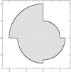 |
Fig. 1. Schematic representation (2D projection) of our ICs for p = 1. |
We then distributed in the ith sector (for i = 1, …, 8) the number of particles that gives the same mean number density in each sector, namely,
 (2)
(2)
The total number of particles is thus  . For the “glass” configurations we extracted a region with the appropriate shape and size from a large glass, a very uniform configuration obtained by running an N-body simulation with a repulsive r−2 force in periodic boundary conditions until an equilibrium configuration is obtained, following a procedure often employed in the generation of “pre-initial” conditions that represent the unperturbed universe for cosmological simulations (Springel 2005).
The limit p = 0 corresponds to spherical symmetry. For p ≠ 0, all rotational symmetry is broken, and the larger p is the more asymmetrical the distribution. We considered here only the range 0 ≤ p ≤ 1. For p > 1, the evolution typically leads to fragmentation into multiple substructures, which then, on a longer timescale, merge together. In this case, the dynamics is thus qualitatively different. In this work we explored up to p = 1, for which the dynamics can be described as a single or a “monolithic” collapse.
We ran simulations for a “grid” of ICs in our two-parameter space: for each of p = 0, 0.2, 0.4, 0.6, 0.8, and 1. The particles are of equal mass and we took N0 in the range 103 − 106. To designate results in the simulations, we used, for given specified p, a label consisting of a letter and an integer. The latter is simply log10N0, while the letter is either S or G: S means that the particles are in a Poisson configuration, and G means that they are in a glass configuration. For example, S4 indicates that the particles were initially Poisson distributed and that N0 = 104. We note that we thus label our simulations by N0, the number of particles inside the inner sphere, and not by the (slightly different) total number of particles. This is appropriate because it allows us to compare simulations at a fixed (or varying) particle density.
Hereafter, distances are given in units of the initial radius of the inner spherical system, R0, and time is given in units of
 (3)
(3)
where M0 is the mass of the inner spherical system and τ0 is the characteristic time corresponding to the time at which the maximal contraction of the system is attained. Virialization occurs a short time later, and in all our simulations the system is well relaxed to a QSS before t = 2 in these units.
We report results for the density profile, ρ(r), normalized by the total mass. Further, we calculate
 (4)
(4)
where ei(t) is the energy of particle i at time t and
 (5)
(5)
is its initial average value. The Δ(t) thus gives a simple measure of the total change of the particle energies relative to the initial time in units of the initial average energy per particle. When Δ(t) > 1, the energy change is large and the collapse is violent, while when Δ(t) < 1 the energy change is small and the collapse is soft (Sylos Labini & Capuzzo-Dolcetta 2020).
Numerical simulations were run using the code Gadget (Springel 2005). We refer to Sylos Labini & Capuzzo-Dolcetta (2020) for further discussion about the details of the numerical integration: Here we just specify that the gravitational softening length was taken to be 1/100 of the minimal radius, rmin, reached by the system during the collapse. We performed numerous tests with smaller and larger softening to check the convergence, finding that results do not depend significantly on ε as long as ε < rmin. Total energy is conserved to a precision better than a few percent; we tested that this is enough to have good convergence of the macroscopic quantities measured here.
3. Results
3.1. Particle energy distributions
The temporal evolution of the particle energy distribution, P(e, t), is a key statistical quantity that characterizes the collapse dynamics (Sylos Labini & Capuzzo-Dolcetta 2020). Figure 2 shows its behavior for the different p simulated for Poisson-distributed particles and N0 = 105 at t = 0 and t = 9 (when, as noted above, the system is very well virialized).
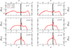 |
Fig. 2. Energy distribution at t = 0 (black line) and at t = 9 (red line) for the series S5; each panel shows a different value of the initial breaking of spherical symmetry, p. |
The trend, which can be seen in Fig. 2, is very clear: In all cases the virialized energy distribution is very different to, and in particular very much broader than, the initial one. However, this difference is greatest at p = 0 and becomes progressively smaller as p increases. This is readily explained by considering that p controls the violence of the collapse: When p = 0, the collapse is close to homologous and the singularity of the N → ∞ limit is regulated only by the density fluctuations seeded by the initial discretization. On the other hand, for p ≠ 0 the collapse is no longer singular in this same limit because tidal effects induced by spatial anisotropies change the collapse times of shells that are initially located at different distances from the center and/or at different angular locations. The larger p is, the more important the effect of these anisotropies in modifying the collapse is and the smaller the change of P(e, t = 9) with respect to P(e, t = 0). One can also see in the plots that there is a small additional peak around e = 0 that appears at p = 0.2 and becomes ever more apparent as p increases. Further, its position (in energy) clearly coincides more closely with the center of the initial distribution as p increases. This feature is evidently a residual of the IC and gives a further quantitative measure of how violent the collapse is.
Next we considered how the N dependence of the energy distributions is obtained from the different ICs. Figure 3 shows P(e, t), again at t = 9, for p = 0 (top panel) and p = 1 (bottom panel) for the different indicated values of N0 and initial Poisson configurations. We observe that while for p = 0 the energy distribution P(e, t = 9) depends strongly on N, for p = 1 there are only very much smaller residual finite N effects. Nevertheless, in the tails of the distribution for p = 1 – for both the most bound and most energetic unbound particles – there appears to still be some systematic dependence on N, with the tails becoming marginally more spread for larger values of N. The convergence to an N-independent result thus seems to be slow, with visible evolution with N still at N0 = 106.
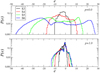 |
Fig. 3. Energy distribution at t = 9 for p = 0 (upper panel) and p = 1 (bottom panel) for the four realizations with a different number of Poisson-distributed particles, i.e., N0 = 103, 104, 105, and 106. |
3.2. Mean energy exchange
The upper panel of Fig. 4 shows the behavior of Δ(t = 9), as defined above in Eq. (4), as a function of p for initial Poisson configurations with different N0. As for P(e, t), the choice of the time t = 9 is somewhat arbitrary as this quantity is essentially time independent provided t ≥ 2. We observe that in all cases Δ > 1, which implies that the collapse is always quite violent in the sense that the variation in the particle energy distribution is large. In a collapse from cold ICs, Δ < 1 can be obtained in the presence of initial fluctuations that are sufficiently large such that clustering proceeds in a bottom-up manner (Sylos Labini & Capuzzo-Dolcetta 2020). We observe that Δ(t = 9) decreases monotonically as a function of p at a fixed value of N0. The behavior simply reflects, once again, that the collapse “softens” progressively as p increases. On the other hand, Δ(t = 9) also increases with N0 at any fixed p, which indicates that the collapse is, in all cases, becoming more violent as N increases. There is, however, a clear weakening of this N dependence as p increases and an apparent onset of good convergence for p = 1 with the two runs with the largest particle numbers close together. Thus, it appears that at p = 1 we attain, at N0 ∼ 105, the limit where the collapse is regulated by the shape fluctuations alone.
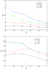 |
Fig. 4. Quantifying the violence of the collapse. Upper panel: energy exchange Δ (see Eq. (4)) at time t = 9 as a function of p (with different N0). Bottom panel: same but the plotted quantity fp is the fraction of ejected particles, i.e., particles that have positive energy after the collapse. |
3.3. Ejected mass
The bottom panel of Fig. 4 shows the fraction of ejected particles, fp, as a function of the initial asymmetry, p, for simulations with N0 = 105. As described in detail in Joyce et al. (2009), Sylos Labini (2012), and Sylos Labini & Capuzzo-Dolcetta (2020), these are essentially all particles whose energy becomes positive in a very short interval around the time of maximal contraction and remains positive thereafter. We note the very large values (approximately one-third of the mass) attained for the spherical IC (see Joyce et al. 2009 for further detail) characterized by the most violent collapse. The behaviors seen are very similar to those in the previous plot, except that there appears to be clearer evidence for convergence with N at the larger values of p.
3.4. Density profiles
Figure 5 shows normalized density profiles, ρ(r), at t = 9 for the indicated simulations. We focus on the very well resolved regions, where r is significantly larger than the gravitational softening. We have multiplied by r4 to facilitate a clearer comparison of the different cases: For the case of p = 0, the outer profile is, as described in previous studies (Joyce et al. 2009; Sylos Labini 2012; Sylos Labini & Capuzzo-Dolcetta 2020), characterized by a radial decay with ρ(r)∼r−4. Both the amplitude of the (flat, approximately constant ρ) core at smaller scales and the amplitude of this tail are strongly N dependent. As discussed in Sylos Labini & Capuzzo-Dolcetta (2020), the exponent −4 corresponds to the limiting situation in which the system is in a Jeans’s equilibrium state; in this state the mass is concentrated in the core, so that the system gravitational potential decays as Φ ∼ r−1 and bound particles in the outskirts move on purely radial orbits (corresponding to an anisotropic velocity parameter β → 1). This configuration is reached only when the collapse is so violent that the potential well of the core becomes very deep and, correspondingly, as seen above, a very significant fraction of mass and energy is ejected, leaving the bound particles with an energy much lower than that of the initial state. If the collapse is much softer, however, the mass distribution is less compact and the gravitational potential decays more slowly than ∼r−1. The particles have less strongly radial orbits as these are a result of the energy ejection around maximal contraction. Figure 5 shows behaviors that are also very consistent with these findings for our ICs. As p increases we see a very apparent transition from an r−4 to an r−3 outer tail in the profile. Further, in line with the previous plots we have analyzed, we see that there appears to be good evidence for convergence with N as one approaches p = 1. At p = 0.6, however, there is still a strong N dependence in both the shape and amplitude of the profile, and it remains unclear what the functional dependence may be as N → ∞.
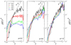 |
Fig. 5. Density profile multiplied by r4 for p = 0 (left panel), p = 0.6 (middle panel), and p = 1 (right panel) obtained from Poisson configurations with different values of N0. The softening length is ε = 3 × 10⁻⁴. The profile for p = 0 is N dependent and decays as r−4; for p = 1 it converges to an N-independent ≈r−3 behavior but is still affected by finite N effects at small scales. A reference line corresponding to ρ(r)∼r−3 is reported in the middle and left panels. |
Figure 6 shows the measured density profile (multiplied by r4) for glass ICs with N0 = 5 × 10⁴ for different values of p. Its behavior is qualitatively the same as what we saw above, with the same apparent transition in the functional form as a function of p. We also find very similar behavior for the other quantities we have analyzed, for both the dependence on p and on N0. There is, however, a quantitative difference between the Poisson and the glass ICs: At given p, the glass ICs with a given N0 closely resemble the Poisson ICs at a slightly larger N0. For instance, a glass IC with N0 ≈ 104 results in a profile that agrees well with that of a Poissonian IC with N0 ≈ 105. This result is completely in line with what was anticipated: At a given N0, the very uniform glass configuration has density fluctuations that are suppressed compared to those of a Poisson configuration. Nevertheless, the quantitative effect, though measurable, is relatively small and our conclusions for what concerns convergence are not changed by our study of these ICs.
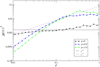 |
Fig. 6. Density profiles multiplied by r4 for simulations with glass ICs and N0 = 5 × 10⁴ for different values of p. Two reference lines with exponents −4 and −3 are also plotted. The softening length is ε = 3 × 10⁻⁴. |
4. Conclusions
We have numerically studied the collapse and virialization of isolated and initially cold configurations of particles with uniform mean density and an irregular asymmetric shape specified by a parameter, p, that characterizes the deviation from sphericity. Such ICs can be considered as a simple schematic representation of the first collapsing regions in cosmological models with a lower cutoff in the spectrum of initial fluctuations. In this context, the number of particles, N, is an unphysical parameter that arises from the N-body discretization, and the model allows us to explore convergence to results that do not depend on it. More generally, the model is a simple toy model for studying how the collapse at finite N in the spherical limit may be modified by deviations from spherical symmetry.
Studying configurations with p in a range where the collapse remains monolithic (i.e., well characterized as a single collapse around a center) and N in the range 103–106, we have been able to see an apparent transition in the qualitative nature of the collapse and the properties of the virialized QSS that result from it. This is most evidently shown by the outer density profile that changes from a power-law decay with an r−4 behavior in the cold spherical limit to a decay with r−3 when the rotational symmetry is broken sufficiently strongly. There are likewise differences that reflect such a transition in the several other various macroscopic quantities we have considered to characterize both the dynamics during the collapse and the final relaxed QSS. The p and N dependence of all these quantities leads to a very coherent interpretation in terms of a competition between the density fluctuations associated with the deviations from spherical symmetry and those associated with the discrete particle distribution. As p increases, the N dependence progressively weakens, and at the largest p there is reasonable evidence for convergence to N-independent results. Nevertheless, residual N dependences are still clearly detectable in some quantities – in the inner parts of the density profile and in the tails of the particle energy distribution – even for the very largest N. In the case of an initially spherical cloud, the transition between a density power-law decay with an r−4 behavior to a decay with r−3 is regulated by density fluctuations (Sylos Labini & Capuzzo-Dolcetta 2020).
In relation to cosmological structure formation, our results qualitatively illustrate two important points. Firstly, they show that a very simple breaking of spherical symmetry in a cold collapse appears to be sufficient to lead to the emergence of an r−3 tail in the virialized state. Such a tail (in the density profiles of halos, i.e., quasi-virialized clumps) is seen very generically in cosmological simulations and has been proposed as a “universal” that is independent of ICs (see, e.g., Navarro et al. 1996). Numerous studies of cold collapse with much more complex ICs than ours have supported such universality (see, e.g., Navarro et al. 2004; Wang et al. 2020), but its origin has remained elusive. Our simple ICs provide a very simplified model for studying this fundamental issue: The nature of the outer profiles of cold dark matter halos is related to both the breaking of spherical symmetry in a cold collapse and the effect of the density fluctuations.
Secondly, our results indicate that the resolution (i.e., particle density) needed to resolve the continuum limit of the first cold collapses predicted in many models of cosmological structure formation may be extremely difficult to reach. Indeed, we have seen that even for quite asymmetric ICs (e.g., corresponding to p = 0.6 in our model) we do not see an approach to convergence of basic macroscopic quantities, even for N = 106 particles. This is many times larger than the typical number of particles inside the first collapsing structures in simulations of warm dark matter models that attempt to model such collapses (Wang & White 2007; Kuhlen et al. 2012). On the other hand, we have seen that the number of particles, N, needed to reach convergence is manifestly strongly dependent on the parameter p, and thus we cannot draw quantitative conclusions for the resolution needed in such cosmological simulations. In future work we plan to address this issue by trying to more precisely model how the breaking of spherical symmetry at the onset of collapse can be characterized and determined in such cosmological models.
Acknowledgments
We are grateful to Lehman Garrison for having provided us the glassy configuration. We thank Roberto Capuzzo Dolcetta, Andrea Gabrielli and Pierfrancesco Di Cintio for useful discussions. Finally, we also thank the referee for his useful comments.
References
- Aarseth, S., Lin, D., & Papaloizou, J. 1988, AJ, 324, 288 [Google Scholar]
- Aguilar, L., & Merritt, D. 1990, AJ, 354, 73 [Google Scholar]
- Arad, I., & Lynden-Bell, D. 2005, MNRAS, 361, 385 [Google Scholar]
- Barnes, E. I., Lanzel, P. A., & Williams, L. L. R. 2009, AJ, 704, 372 [Google Scholar]
- Benhaiem, D., Joyce, M., Sylos Labini, F., & Worrakitpoonpon, T. 2016, A&A, 585, A139 [NASA ADS] [CrossRef] [EDP Sciences] [Google Scholar]
- Benhaiem, D., & Sylos Labini, F. 2015, MNRAS, 448, 2634 [Google Scholar]
- Benhaiem, D., & Sylos Labini, F. 2017, A&A, 598, A95 [CrossRef] [EDP Sciences] [Google Scholar]
- Boily, C. M., & Athanassoula, E. 2006, MNRAS, 369, 608 [Google Scholar]
- Boily, C., Athanassoula, E., & Kroupa, P. 2002, MNRAS, 332, 971 [Google Scholar]
- Henon, M. 1964, A&A, 27, 1 [Google Scholar]
- Henon, M. 1973, A&A, 24, 229 [Google Scholar]
- Joyce, M., Marcos, B., & Sylos Labini, F. 2009, MNRAS, 397, 775 [NASA ADS] [CrossRef] [Google Scholar]
- Kuhlen, M., Vogelsberger, M., & Angulo, R. 2012, Phys. Dark Universe, 1, 50 [Google Scholar]
- Lin, C. C., Mestel, L., & Shu, F. H. 1965, AJ, 142, 1431 [Google Scholar]
- Lynden-Bell, D. 1967, MNRAS, 136, 101 [NASA ADS] [CrossRef] [Google Scholar]
- Mangalam, A., Nityananda, R., & Sridhar, S. 1999, AJ, 524, 623 [Google Scholar]
- Merritt, D., & Aguilar, L. A. 1985, MNRAS, 217, 787 [Google Scholar]
- Navarro, J. F., Eke, V. R., & Frenk, C. S. 1996, MNRAS, 283, L72 [NASA ADS] [Google Scholar]
- Navarro, J. F., Hayashi, E., Power, C., et al. 2004, MNRAS, 349, 1039 [NASA ADS] [CrossRef] [Google Scholar]
- Peebles, P. J. E. 1980, The Large-Scale Structure of the Universe (Princeton, NJ: Princeton University Press) [Google Scholar]
- Roy, F., & Perez, J. 2004, MNRAS, 348, 62 [Google Scholar]
- Spera, M., & Capuzzo-Dolcetta, R. 2017, Astrophys. Space Sci., 362, 233 [Google Scholar]
- Springel, V. 2005, MNRAS, 364, 1105 [Google Scholar]
- Sylos Labini, F. 2012, MNRAS, 423, 1610 [Google Scholar]
- Sylos Labini, F. 2013, MNRAS, 429, 679 [Google Scholar]
- Sylos Labini, F., & Capuzzo-Dolcetta, R. 2020, A&A, 643, A118 [EDP Sciences] [Google Scholar]
- Sylos Labini, F., Benhaiem, D., & Joyce, M. 2015, MNRAS, 449, 4458 [Google Scholar]
- Sylos Labini, F., Pinto, L. D., & Capuzzo-Dolcetta, R. 2020, Phys. Rev. E, 102 [Google Scholar]
- Theis, C., & Spurzem, R. 1999, A&A, 341, 361 [NASA ADS] [Google Scholar]
- van Albada, T. 1982, MNRAS, 201, 939 [Google Scholar]
- Wang, J., & White, S. D. M. 2007, MNRAS, 380, 93 [NASA ADS] [CrossRef] [Google Scholar]
- Wang, J., Bose, S., Frenk, C. S., et al. 2020, Nature, 585, 39 [Google Scholar]
- Worrakitpoonpon, T. 2015, MNRAS, 466, 1335 [Google Scholar]
- Worrakitpoonpon, T. 2020, MNRAS, 498, 310 [Google Scholar]
All Figures
|
Fig. 1. Schematic representation (2D projection) of our ICs for p = 1. |
| In the text | |
|
Fig. 2. Energy distribution at t = 0 (black line) and at t = 9 (red line) for the series S5; each panel shows a different value of the initial breaking of spherical symmetry, p. |
| In the text | |
|
Fig. 3. Energy distribution at t = 9 for p = 0 (upper panel) and p = 1 (bottom panel) for the four realizations with a different number of Poisson-distributed particles, i.e., N0 = 103, 104, 105, and 106. |
| In the text | |
|
Fig. 4. Quantifying the violence of the collapse. Upper panel: energy exchange Δ (see Eq. (4)) at time t = 9 as a function of p (with different N0). Bottom panel: same but the plotted quantity fp is the fraction of ejected particles, i.e., particles that have positive energy after the collapse. |
| In the text | |
|
Fig. 5. Density profile multiplied by r4 for p = 0 (left panel), p = 0.6 (middle panel), and p = 1 (right panel) obtained from Poisson configurations with different values of N0. The softening length is ε = 3 × 10⁻⁴. The profile for p = 0 is N dependent and decays as r−4; for p = 1 it converges to an N-independent ≈r−3 behavior but is still affected by finite N effects at small scales. A reference line corresponding to ρ(r)∼r−3 is reported in the middle and left panels. |
| In the text | |
|
Fig. 6. Density profiles multiplied by r4 for simulations with glass ICs and N0 = 5 × 10⁴ for different values of p. Two reference lines with exponents −4 and −3 are also plotted. The softening length is ε = 3 × 10⁻⁴. |
| In the text | |
Current usage metrics show cumulative count of Article Views (full-text article views including HTML views, PDF and ePub downloads, according to the available data) and Abstracts Views on Vision4Press platform.
Data correspond to usage on the plateform after 2015. The current usage metrics is available 48-96 hours after online publication and is updated daily on week days.
Initial download of the metrics may take a while.