| Issue |
A&A
Volume 652, August 2021
|
|
|---|---|---|
| Article Number | A149 | |
| Number of page(s) | 8 | |
| Section | Planets and planetary systems | |
| DOI | https://doi.org/10.1051/0004-6361/202039556 | |
| Published online | 26 August 2021 | |
Constraining the nature of the possible extrasolar PDS110b ring system
Grupo de Dinâmica Orbital e Planetologia, São Paulo State University, UNESP,
Guaratinguetá, CEP
12516-410,
São Paulo,
Brazil
e-mail: This email address is being protected from spambots. You need JavaScript enabled to view it.
; This email address is being protected from spambots. You need JavaScript enabled to view it.
Received:
29
September
2020
Accepted:
17
June
2021
Abstract
The young star PDS110 in the Ori OB1a association underwent two similar eclipses in 2008 and 2011, each of which lasted for a period of at least 25 days. One plausible explanation for these events is that the star was eclipsed by an unseen giant planet (named PDS110b) circled by a ring system that fills a large fraction of its Hill sphere. Through thousands of numerical simulations of the three-body problem, we constrain the mass and eccentricity of this planet as well the size and inclination of its ring, parameters that are not well determined by the observational data alone. We carried out a broad range of different configurations for the PDS110b ring system and ruled out all that did not match with the observations. The result shows that the ring system could be prograde or retrograde; the preferred solution is that the ring has an inclination lower than 60° and a radius between 0.1 and 0.2 au and that the planet is more massive than 35 MJup and has a low eccentricity (<0.05).
Key words: planets and satellites: rings / planets and satellites: dynamical evolution and stability / eclipses
© ESO 2021
1 Introduction
The first exoplanet discovered was around a pulsar, PSR1257+12 (Wolszczan & Frail 1992), and three years later the first detection of a planet (51 Pegasi b) orbiting a solar-type star occurred (Mayor & Queloz 1995). In our Solar System, all four giant planets host ring systems; however, as of now, no extrasolar ring system (exoring) has been detected, and the detection of a Saturn-like ring system requires high time-resolution photometry (Barnes & Fortney 2004). The most useful method for detecting the presence of a ring is the planetary transit (Akinsanmi et al. 2020), and several works have searched for signatures of a planetary ring system around extrasolar Kepler planet candidates (e.g., Heising et al. 2015, and Aizawa et al. 2017, 2018).
Schlichting & Chang (2011) analyzed the nature of possible ring systems that could exist around an exoplanet with an orbital period of about one year or less. Their results show that 24% of the evaluated planets have the necessary conditions to support sizable rings, and, since these planets would be very close to their host star, the orbiting disk around them probably consists of rocky material.
The first exoring candidate was reported in 2007, when the star J1407 underwent a complex series of eclipses that lasted about 56 days and achieved a depth greater than three magnitudes (Mamajek et al. 2012). One potential solution for this event is the passage of a giant ring that extends out to a radius of 0.6 au, surrounding an unseen secondary companion that is in front of the star. The structure has a gap at 0.4 au, which, according to Kenworthy & Mamajek (2015), could be a result of an exomoon clearing out this region. This exosatellite is expected to have a mass comparable to that of the Earth. Rieder & Kenworthy (2016) investigated, through numerical simulation, the effect on the stability of the ring system around J1407b in an eccentric orbit (0.6 ≤ e ≤ 0.7) and with an orbital period of 11 yr. The results strongly suggest that a retrograde ring and a secondary companion with a mass of 60–100 MJup can fit the observable eclipse.
Speedie & Zanazzi (2020) investigated the stability and structure of a circumplanetary ring system around an oblate and oblique planet under the influence of the spinning planet’s mass quadrupole coefficient (J2) through N-body integrations. Their results show that a massive planet (10 MJup) orbiting a Sun-like star either in circular or eccentric orbit can wrap a stable ring that extends out to a 2 Laplace radius. The authors identified two main instability mechanisms. The first is the Lidov-Kozai instability, which occurs for a planet with an obliquity of 80°, and the second is ivection instability. Even though there is no measurement of the oblateness coefficient, they assumed J2 = 0.5 for J1407b (30 times larger than Saturn’s), finding that the likely mass for the planet is greater than 13 MJup.
Another possible exoring structure was found in the PDS110 system. The young star PDS110 (~11 Myr old), which is roughly two times more massive than the Sun, underwent two series of eclipses in 2008 and 2011, with each dimming event lasting about 25 days with a depth of 30%. The infrared excess in the total luminosity of PDS110 indicates the presence of a dust disk encircling the star, and the similarity between the events suggests the presence of a periodic unseen secondary companion surrounded by a circum-secondary disk structure (Osborn & Rodriguez 2017). Another eclipse was predicted to happen in 2017, and a ground-based observing campaign was organized to monitor the event. However, no drop greater than 1% was detected. Osborn & Kenworthy (2019) propose that, instead of a ring, a circumstellar dust disk around PDS110 could be the source of variability. Future observations can confirm the existence of this ring system and the secondary companion.
A number of characteristics of the secondary companion could not be well determined from the observations. Osborn & Rodriguez (2017) reported that the hypothetical companion orbits the PDS110 star at 2 au and that its mass is in the range of [1.8–70] MJup, which would indicate it is a planet or a brown dwarf. The presumed ring would have a radius of about 0.15 au.
The goal of this work is to analyze the stability of a putative exoring system around an eccentric, massive planet at 2 au from the PDS110 star that matches with the eclipses that occurred in 2008 and 2011. Given the extensive range of possible values for a planet’s mass and eccentricity, ring size, and inclination, we aim to restrict the physical and orbital parameters of this system through numerical simulation.
In Sect. 2 we describe in detail the ring system and the two main eclipses. In Sect. 3 we present the first constraints on the upper limit for the eccentricity of the planet, while in Sect. 4 we report the numerical model for the putative systems, exploring different values for the mass and eccentricity of the planet and for the orbital inclination of the ring. The results of the numerical simulations are discussed in Sect. 5, for both prograde and retrograde cases. Our final remarks are presented in the last section.
2 The PDS110b ring system
The star PDS110, also identified as IRAS 05209-0107 or HD 290380, is an ~11 Myr old GE/FE-type star and a member of the Ori OB1a association at a distance of 345 ± 40 pc (Brown et al. 2016). It has a radius roughly equivalent to the diameter of the Sun (2.23 R⊙) and a mass ~1.6 times the solar mass. The presence of infrared excess, approximately 25% of the total luminosity (LIR ∕Lbol = 0.25; Osborn & Rodriguez 2017), indicates the presence of two protoplanetary disks surrounding the star: an inner one with an extension of approximately 0.2 au, too small to be directly detected by images, and a second inclined outer disk, formed by dust with an extension of up to 300 au.
The PDS110 system underwent two similar dimming events, each over 25 days and with a brightness drop of ~30%. The events were observed in 2008 and 2011, as reported by Osborn & Rodriguez (2017) and Osborn & Kenworthy (2019). An analysis by Osborn & Rodriguez (2017) investigated two different interpretations for the eclipses. The first possible explanation was the passage of an inclined disk around an unseen low mass secondary companion, possibly a brown dwarf or a giant planet. The authors concluded that any large disk around PDS110 would have been detected in the optical spectra, as would any indication of a secondary star in the system. The second and more probable explanation for the eclipses is that a circumplanetary disk around PDS110b caused them.
The interval of two years between eclipses suggests an orbital period for the secondary companion of 808 days. Considering that the mass of the star is 1.6 M⊙, the estimated semimajor axis of PDS110b would be ~2 au. An analytical analysis of the eclipse made by Osborn & Rodriguez (2017), assuming a circular orbit for the planet, implies that the secondary companion may have a mass between 1.8 and 70 MJup. Furthermore, from the orbital speed and eclipse duration, and assuming the secondary has a circular orbit, the authors estimated the disk diameter to be around 0.3 au. Based on the observational data, no constraint on the planet eccentricity was made.
Here we explore the case that the secondary body is a planet (hereafter called PDS110b) that hosts an extensive ring system that was invisible during the eclipses. Our goal is to better constrain the physical and orbital parameters of the PDS110b system through numerical simulations and some analytical analysis in order to explain the dimming events.
3 Constraints on the eccentricity of PDS110b
Initially, we performed an analytic analysis to constrain an upper limit for the eccentricity of PDS110b by correlating the ring orbital radius with the Hill region of the planet.
The Hill radius (rHill) is the distance from the planet where the gravitational influence of the host planet dominates over the stellar perturbation. In the case of an eccentric orbit, the Hill radius can be estimated as (Hamilton & Burns 1992)
![Mathematical equation: \begin{align*}r_{\mathrm{Hill}} \approx a (1 - e) \sqrt[3]{\frac{m_{\mathrm{p}}}{3 M_{\mathrm{s}}}},\end{align*}](/articles/aa/full_html/2021/08/aa39556-20/aa39556-20-eq1.png) (1)
(1)
where a is the semimajor axis, e is the eccentricity, and mp and Ms are the masses of the planet and the star, respectively.
Since the disk inclination and the planet obliquity are unknown, we assume the ring inclination observed from Earth is 0° (face-on) and that the ring is in the equatorial plane of the planet. Now let te be the eclipse duration time, assuming the planet travels in a straight line with a constant velocity ve. The radial size of the projected ring, rring, can be written as
 (2)
(2)
and the two parameters can be combined to define ξ as the ratio between the ring and the Hill radius
 (3)
(3)
which helps us understand the stability of the ring.
We considered the mass of the star to be Ms = 1.6 M⊙, the observed period of the planet to be P = 808 days, and the eclipse to last te = 25 days. To explore an extreme configuration, we assumed the ring to be in the orbital plane of the planet and the eclipse to happen during the passage of the planet through the apocenter (when the planet velocity is at its minimum). With these assumptions, ξ was calculated for the secondary companion mass in the range of [1.8–70] MJup (Osborn & Rodriguez 2017) and for different values of eccentricity.
If ξ < 1, the ring is within the gravitational domain of the planet. Hunter (1967) studied the stability orbits of hypothetical satellites around Jupiter disturbed by the Sun, with different values for the semimajor axis, eccentricity, and inclination. Their results showed that the stability region for prograde orbits is smaller than 0.45 rHill, while for retrograde orbits the extension of this region is limited to 0.75rHill. Domingos et al. (2006) studied the stability zone of satellites around extrasolar giant planets and verified that the limit of the stable region is ~ 0.5 rHill for prograde orbits and around ~0.95 rHill for the retrograde case (they restricted the analysis to a mass ratio between the massive bodies of a maximum of 10−3). Therefore, in our analysis we consider systems to be stable when ξ < 0.5.
Figure 1 shows ξ as a function of the mass of the planet for different values of the planet’s eccentricity (ep). The horizontal line corresponds to the stability limit of ξ = 0.5, allowing us to constrain the mass of the planet to be greater than 35 MJup and to rule out systems where the eccentricity of the planet is larger than 0.5.
The high eccentricity implies that the planet transit velocity is greater than 15 km s−1, which is consistent with the minimal eclipse velocity detected by Osborn & Rodriguez (2017) through observational data. From the flux increase in the light curve, they calculated the minimum velocity of the object during the event to be vmin = 13 km s−1.
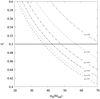 |
Fig. 1 Factor ξ in terms of planet mass (mp) and its eccentricity (ep). The line at ξ = 0.5 delineates the stability zone (which is below this line). |
4 Numerical method
To investigate the possible physical and orbital parameters of the PDS110b ring system, we numerically modeled the system as an ensemble of three-body problems: the star, a planet, and the ring particle, where each numerical simulation represents one different initial condition of the system. In total, we ran 1.3 × 10⁶ different simulations.
For all models, we set the values of PDS110 and its companion, PDS110b, to be in agreement with the values from Osborn & Rodriguez (2017). The mass of the star is 1.6 M⊙, and its radius is 2.23 M⊙. The parameters of the hypothetical planet were assumed considering the following grid of parameters: The semimajor axis (ap) is fixed to 2 au, while the eccentricity (ep) and the mass (mp) are randomly chosen within the ranges of 0 to 0.5 and 1.8–70 MJup, respectively.These intervals were determined based on the references presented in Sect. 2; however, for the sake of completeness, we decided to analyze the entire mass range proposed in Osborn & Rodriguez (2017). The radius of the planet (rp) was calculated assuming a density of 1.326 kg m−3 (the same as Jupiter’s).
We considered the ring particle as a test particle orbiting the planet and gravitationally perturbed by the star. The particle is initially in a circular orbit, and the semimajor axis (a) is chosen randomly from the range 0.01 to 0.5 au and the true anomaly (f) from 0° to 360°. We assumed the other parameters of the particles, the longitude of the ascending node (Ω) and the argument of pericenter (ω), to be 0°. Assuming the possibility that the eclipses occurred via an inclined ring (Osborn & Rodriguez 2017), we varied, for each set of 105 numerical simulations, the inclination of the particle (i), defined as the angle between the ring plane and the orbital planet of the planet, from 0° to 180° in steps of Δi = 15°.
The time span for all numerical simulations was set as 250 × 104 days, the equivalent of 104 orbital periods of the particle with a semimajor axis a = 0.5 au and orbiting a planet with a mass of 1.8 MJup. Among all the possible scenarios, this is the largest period that one particle could have. The numerical integrations were carried out with the Rebound package using the IAS15 integrator (Rein & Spiegel 2014).
Whenever the particle collided with one of the massive bodies or was ejected from the system, the simulation was interrupted. The collisions were defined when the distance between the particle and a massive body (star or planet) was smaller than the body’s radius, and particles were considered ejected when their orbit became hyperbolic (e < 1) in reference to the planet. All the particles that survived the entire time of integration were considered to be stable.
We divided our set of simulations into 1820 different groups according to the inclination of the ring particle, theeccentricity, and the mass of the planet, by grouping them within the following intervals: Δi = 15°, Δep = 0.05, and Δmp≈ 5 MJup. For each set, we determined the radial distribution of the surviving particles throughout the entire integration. To remove outliers, the ring extension (rring) in each group was defined as the semimajor axis distance from the farthest particle within the area where the nearest 98% of the ensemble remained.
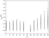 |
Fig. 2 Ring radius of each group of simulations based on a ring inclination from i = [0° to 180°]. |
5 Numerical results
Given the large number of variables, we explored thousands of different sets of initial conditions within the ranges described inSect. 4. For the complete ensemble, the overall outcome was as follows: 6.3% of the cases ended in collision and 72.2% ended in escape, while in the remaining 21.5% of the cases the particles remained stable throughout the entire integration. It is interesting to note that the majority of the unstable particles (~93%) were ejectedor collided with one of the massive bodies in less than 40 orbital periods of the planet (<80 yr).
We also verified the relation between the orbital inclination of the particle and the ring radius (Fig. 2). Each dot represents a group of simulations. We see that the ring extension varies largely depending on the inclination, going from less than 0.05 au for the smallest scenario up to almost 0.4 au.
When the inclination is 90°, all particles are unstable, regardless of the mass of the planet. The figure also shows that the range of the ring size increases for larger inclinations. For prograde rings (i < 90°) the maximum extension is around 0.22 au, while for retrograde rings, where the systems are more stable, the ring reaches 0.38 au in radius.
The numerical results presented in Figs. 3 and 4 (prograde and retrograde cases, respectively) are the diagrams of the particles’ semimajor axis (a) versus particle eccentricity (e) for the stable particles. Each plot represents systems with different planet masses but the same ring inclination.
The initially circular ring particles quickly became eccentric, and this effect is more prominent for highly inclined rings. Figure 3 shows that for i≤ 30° (panels a to c) the majority of particles are found within e < 0.3 and a < 0.2 au. For i = 45° the stable particles are mostly confined to e ≤ 0.4 and a ≤ 0.2 au. In the range of i = [60°, 75°], a significant number of particles present large eccentricities, reaching values close to unity with a ≤ 0.22 au.
No stable particle is found with an inclination around 90°. In the retrograde case (Fig. 4), for i = 105° the maximum semimajor axis distance of the stable region is around 0.13 au, and these values increase when the ring inclination is 180°, reaching as high as a ~ 0.4 au. The maximum particle eccentricity decreases as the ring inclination rises: The value of e goes from almost 1 for i = 105° (Fig. 4a) to e ≤ 0.7 for i = 180° (Fig. 4f).
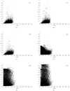 |
Fig. 3 Set of diagrams: the semimajor axis versus the eccentricity of the stable particles (in black) for the prograde case. In the different plots the ring particle inclination is: (a) 0°; (b) 15°; (c) 30°; (d) 45°; (e) 60°; and (f) 75°. |
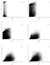 |
Fig. 4 Set of diagrams: the semimajor axis (a) versus the eccentricity of the stable particles (in black) for the retrograde case. The ring particle inclination is: (a) 105°; (b) 120°; (c) 135°; (d) 150°; (e) 165°; and (f) 180°. The diagramfor i = 90° is missing because no stable region exists in this case. |
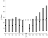 |
Fig. 5 Eclipse duration for different ring system inclinations. Each vertical bar represents the possible duration of the eclipses for a given inclination assuming the different ring extensions. The dot indicates the average value of each box, and the dashed line represents the observed eclipse (25 days). |
5.1 Eclipse duration
For each group of simulations, we calculated the theoretic eclipse time (te) according to Eq. (2), always assuming a face-on configuration. To identify the physical and orbital parameters of the PDS110b system from the numerical results, we assumed the planet semimajor axis to be 2 au and its orbital period to be 808 days. We considered the ring radius to be the semimajor axis of the most distant particle and considered the planet velocity derived in two different positions of its orbit, at pericenter and apocenter (extreme cases).
The interval of all possible theoretical eclipse times (te) for each group of simulations is presented in Figs. 5–11. In each plot the horizontal line corresponds to the observed eclipse duration (25 days), thus indicating which configurations (planet mass and eccentricity, ring extension, and inclination) for the PDS110b ring system could reproduce the observed events.
Figure 5 shows that both prograde and retrograde ring systems may explain the transit events when considering orbital inclinations smaller than60° or higher than 120°. In the rangei = [75°−105°] the stable ring is not large enough to reproduce an eclipse that matches the observation. We now divide the discussion into two sections, theprograde and retrograde cases.
5.2 Prograde case
Out of our set of 1820 groups of simulations, half correspond to prograde orbits of the planet. In this case, the ring inclination is required to be smaller than 60° to produce an eclipse that lasts 25 days. It is most likely that in these systems the mass of the secondary companion is larger than 35 MJup (Fig. 6), which is consistent with the results presented in Fig. 3.
It is also possible to group the ring extension for the simulated systems according to the eccentricity of the planet (Fig. 7). Assuming the eclipse occurred at the apocenter of the planet, any eccentricity ep < 0.3 is possible. However, if we consider that the eclipse took place at the pericenter, only a planet with a circular or slightly eccentric orbit (ep < 0.05) could have a disk capable of consistently explaining the transit time, suggesting that a planet with a lower eccentricity is more plausible.
Planets with a higher eccentricity present a less extensive ring system, and this directly influences the eclipse duration. This is expected since the planet is reasonably close to the star (2 au) and since the outermost particles are increasingly perturbed by the star as the orbit becomes more eccentric.
We computed the eclipse duration for each of the 910 prograde cases, assuming that the planet is either in the pericenter or the apocenter (Fig. 8). Given that the velocity of the planet is maximum at the pericenter, the planet requires a ring with an extension of ~ 0.2 au to produce a 25-day eclipse when viewed face-on. Conversely, at the apocenter (thus, at a lower velocity), a ring extension from 0.1 to 0.2 au matches the observation. This range corresponds to less than 0.5 rHill, which is compatible with previous works.
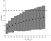 |
Fig. 6 Influence of the mass of the planet on the eclipse time, for prograde systems. The rectangles indicate the duration of the possible eclipses within a specific mass range, grouped every Δmp ≈ 5 MJup. |
5.3 Retrograde case
Retrograde systems can also sustain a ring that is large enough to be consistent with a transit that lasts 25 days. In fact, given the more extensive distribution of stable particles (see Fig. 4), more retrograde systems fit the eclipse than prograde orbit systems. When grouping the simulations according to the mass of the planet (Fig. 4), we see that only systems where mp < 5 MJup cannot explain the eclipse.
Regarding the possible eccentricities of the planet, if the eclipse happens at the apocenter (right panel in Fig. 10), any value smaller than 0.5 is allowed. However, at the pericenter, where the orbital velocity is at its maximum, only systems with a smaller eccentricity (ep < 0.25) are plausible solutions.
Figure 11 shows the eclipse time as a function of the ring extension of each retrograde system. In this case, the eclipse could be explained by some systems with a ring radius from 0.1 au up to 0.25 au, depending on whether we assume the eclipse happens at the pericenter or apocenter of the planetary orbit. Due to the stability of the retrograde system, the size of the ring could be much larger than what is necessary to explain the eclipse, reaching almost 0.4 au (~ 0.95 rHill) in extreme cases.
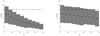 |
Fig. 7 Time span of the duration of the eclipses for a prograde ring grouped according to the eccentricity of the planet (ep). Panel on the left: the eclipse is occurring at the pericenter. Right: the eclipse is occurring during the planet passage at the apocenter. The dashed line represents the observable eclipse (25 days). |
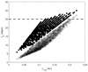 |
Fig. 8 Eclipse time according to the ring radius for planets with a prograde orbit. The eclipse duration changes if it is assumed that the event occurs at the pericenter of the orbit (open circles) or the apocenter (filled circles). The dashed line indicates the observed eclipse. |
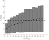 |
Fig. 9 Influence of the mass of the planet on the eclipse time, for retrograde systems. The rectangles indicate the duration of the possible eclipses within a specific mass range, grouped every Δmp ≈ 5 MJup. |
6 Final comments
The two eclipses of the star PDS110 in 2008 and 2011 were initially interpreted as results of the transit of the edge of a gigantic and inclinedring (Osborn & Rodriguez 2017). This ring could be around an unseen secondary companion, either a brown dwarf or a giant planet (named PDS110b). This secondary would be 2 au from the star, with a mass > 1.8 MJup. No other constraints on the system could be made through the observational data.
We proposed to find possible limits on the mass and eccentricity for the secondary body, as well as the ring radius and inclination that could produce an equivalent transit duration assuming we have a face-on view of the system. To do so, we performed numerical simulations, assigning random values for the parameters of the system within the ranges derived from the observations.
Initially, we found that the limit of the stability zone for a circumplanetary disk sets the maximum eccentricity of the planet as 0.5, which is in agreement with an analytical approach. If the planet is more eccentric, the ring is more disturbed by the star, and its size is not large enough to create a 25-day eclipse.
We also simulated rings with inclinations from 0° to 180°. The largest prograde stable ring system we found filled a fraction of ~0.5 rHill, compatible with theoretical studies. In retrograde simulations, this stability zone can extend to almost one Hill radius (~ 0.95 rHill).
The approach we followed to determine the stability resulted in a large ring and cannot be directly compared to the method presented by Speedie & Zanazzi (2020). Our instability criteria rely on ejection or collision, while their analysis is related to a torque balance between the tidal torques from the star and a planet, and they also have a stricter stability classification related to the variation in the inclination and eccentricity of the particle. Furthermore, the torque from the planet is directly dependent on the J2 coefficient, which is an unknown parameter for the PDS110b and would introduce an extra degree of freedom in our analysis.
The eclipse duration depends on the orbital velocity of the planet. Thus, we computed the extreme cases for transit at the pericenter and at the apocenter, both for prograde and retrograde ring systems. When the ring inclination is smaller than 90°, it requires a more massive planet (mp > 35 MJup) and its eccentricity is limited to 0.2 for transit at the pericenter. If the eclipse occurs at the apocenter, any value of ep < 0.5 could explain the eclipse. In a retrograde configuration, the imposed constraints are looser since the eclipse could be explained for systems with mp > 5 MJup.
Although the retrograde ring system may have a broader range of possible configurations to explain the eclipse, we consider a prograde system to be more likely since it is hard to justify the origin of such a large ring (~0.2 au) in retrograde motion. In our Solar System, we do not have any example of a retrograde ring system, just some irregular moons of Jupiter, Saturn, and Neptune; in these cases, the moons were captured into orbit by the planet’s gravity.
In summary, the most likely result from our simulations is the configuration for the PDS110b system with a ring radius in the range [0.1–0.2] au and an inclination i < 60°. The planet probably has a small eccentricity (e < 0.05) and is probably very massive mp > 35 MJup.
It is worth recalling that we assumed that we are always observing the system face-on in our analysis. If the disk is inclined in the sky plane, the observed radial extension of the ring is reduced, and therefore many of the possible configurations that we considered acceptable vanish.
Since the results we present are derived from numerical simulations carried out for more than 6000 yr (104 orbital periods), it is beyond the scope our analysis to explain why the predicted dimming event in 2017 was negative after two positive detections in 2008 and 2011. Osborn & Kenworthy (2019) argued that these eclipses might be some aperiodic event and not related to the transit of an exoring.
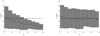 |
Fig. 10 Time span of the duration of the eclipses for a retrograde system according to the eccentricity of the planet (ep). Panel on the left: the eclipse is occurring at the pericenter. Right: during the planet passage at the apocenter. |
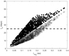 |
Fig. 11 Eclipse time according to the ring radius for planets with a retrograde orbit. The eclipse duration changes if it is assumed that the event occurs at the pericenter of the orbit (open circles) or the apocenter (filled circles). The dashed line indicates the observed eclipse. |
Acknowledgements
The authors are grateful to the anonymous referee that contributed significantly to the improvement of the paper. This research was financed in part by the Coordenação de Aperfeiçoamento de Pessoal de Nível Superior - Brasil (CAPES) - Finance Code 001, and Fundação de Amparo a Pesquisa no Estado de São Paulo (FAPESP) Proc. 2016/24561-0.
References
- Aizawa, M., Uehara, S., Masuda, K., Kawahara, H., & Suto, Y. 2017, AJ, 153, 193 [Google Scholar]
- Aizawa, M., Masuda, K., Kawahara, H., & Suto, Y. 2018, AJ, 155, 206 [NASA ADS] [CrossRef] [Google Scholar]
- Akinsanmi, B., Santos, N., Faria, J., et al. 2020, A&A, 635, L8 [Google Scholar]
- Barnes, J. W., & Fortney, J. J. 2004, AJ, 616, 1193 [Google Scholar]
- Brown, A. G., Vallenari, A., Prusti, T., et al. 2016, A&A, 595, A2 [Google Scholar]
- Domingos, R. C., Winter, O. C., & Yokoyama, T. 2006, MNRAS, 373, 1227 [Google Scholar]
- Hamilton, D. P., & Burns, J. A. 1992, Icarus, 96, 43 [Google Scholar]
- Heising, M., Marcy, G., & Schlichting, H. 2015, ApJ, 814, 81 [Google Scholar]
- Hunter, R. 1967, MNRAS, 136, 245 [Google Scholar]
- Kenworthy, M. A., & Mamajek, E. E. 2015, ApJ, 800, 126 [NASA ADS] [CrossRef] [Google Scholar]
- Mamajek, E. E., Quillen, A. C., Pecaut, M. J., et al. 2012, AJ, 143, 72 [Google Scholar]
- Mayor, M., & Queloz, D. 1995, Nature, 378, 355 [Google Scholar]
- Osborn, H. P., & Kenworthy, et al. 2019, MNRAS, 485, 1614 [Google Scholar]
- Osborn, H. P., & Rodriguez, et al. 2017, MNRAS, 471, 740 [Google Scholar]
- Rein, H., & Spiegel, D. S. 2014, MNRAS, 446, 1424 [Google Scholar]
- Rieder, S., & Kenworthy, M. A. 2016, A&A, 596, A9 [Google Scholar]
- Schlichting, H. E., & Chang, P. 2011, AJ, 734, 117 [Google Scholar]
- Speedie, J., & Zanazzi, J. 2020, MNRAS, 497, 1870 [Google Scholar]
- Wolszczan, A., & Frail, D. A. 1992, Nature, 355, 145 [NASA ADS] [CrossRef] [Google Scholar]
All Figures
|
Fig. 1 Factor ξ in terms of planet mass (mp) and its eccentricity (ep). The line at ξ = 0.5 delineates the stability zone (which is below this line). |
| In the text | |
|
Fig. 2 Ring radius of each group of simulations based on a ring inclination from i = [0° to 180°]. |
| In the text | |
|
Fig. 3 Set of diagrams: the semimajor axis versus the eccentricity of the stable particles (in black) for the prograde case. In the different plots the ring particle inclination is: (a) 0°; (b) 15°; (c) 30°; (d) 45°; (e) 60°; and (f) 75°. |
| In the text | |
|
Fig. 4 Set of diagrams: the semimajor axis (a) versus the eccentricity of the stable particles (in black) for the retrograde case. The ring particle inclination is: (a) 105°; (b) 120°; (c) 135°; (d) 150°; (e) 165°; and (f) 180°. The diagramfor i = 90° is missing because no stable region exists in this case. |
| In the text | |
|
Fig. 5 Eclipse duration for different ring system inclinations. Each vertical bar represents the possible duration of the eclipses for a given inclination assuming the different ring extensions. The dot indicates the average value of each box, and the dashed line represents the observed eclipse (25 days). |
| In the text | |
|
Fig. 6 Influence of the mass of the planet on the eclipse time, for prograde systems. The rectangles indicate the duration of the possible eclipses within a specific mass range, grouped every Δmp ≈ 5 MJup. |
| In the text | |
|
Fig. 7 Time span of the duration of the eclipses for a prograde ring grouped according to the eccentricity of the planet (ep). Panel on the left: the eclipse is occurring at the pericenter. Right: the eclipse is occurring during the planet passage at the apocenter. The dashed line represents the observable eclipse (25 days). |
| In the text | |
|
Fig. 8 Eclipse time according to the ring radius for planets with a prograde orbit. The eclipse duration changes if it is assumed that the event occurs at the pericenter of the orbit (open circles) or the apocenter (filled circles). The dashed line indicates the observed eclipse. |
| In the text | |
|
Fig. 9 Influence of the mass of the planet on the eclipse time, for retrograde systems. The rectangles indicate the duration of the possible eclipses within a specific mass range, grouped every Δmp ≈ 5 MJup. |
| In the text | |
|
Fig. 10 Time span of the duration of the eclipses for a retrograde system according to the eccentricity of the planet (ep). Panel on the left: the eclipse is occurring at the pericenter. Right: during the planet passage at the apocenter. |
| In the text | |
|
Fig. 11 Eclipse time according to the ring radius for planets with a retrograde orbit. The eclipse duration changes if it is assumed that the event occurs at the pericenter of the orbit (open circles) or the apocenter (filled circles). The dashed line indicates the observed eclipse. |
| In the text | |
Current usage metrics show cumulative count of Article Views (full-text article views including HTML views, PDF and ePub downloads, according to the available data) and Abstracts Views on Vision4Press platform.
Data correspond to usage on the plateform after 2015. The current usage metrics is available 48-96 hours after online publication and is updated daily on week days.
Initial download of the metrics may take a while.