| Issue |
A&A
Volume 652, August 2021
|
|
|---|---|---|
| Article Number | A152 | |
| Number of page(s) | 14 | |
| Section | Cosmology (including clusters of galaxies) | |
| DOI | https://doi.org/10.1051/0004-6361/202038106 | |
| Published online | 26 August 2021 | |
Correlation functions in 2D and 3D as descriptors of the cosmic web
1
Tartu Observatory, 61602 Tõravere, Estonia
e-mail: jaan.einasto@ut.ee
2
Estonian Academy of Sciences, 10130 Tallinn, Estonia
3
ICRANet, Piazza della Repubblica 10, 65122 Pescara, Italy
4
National Institute of Chemical Physics and Biophysics, Tallinn 10143, Estonia
Received:
7
April
2020
Accepted:
24
May
2021
Aims. Our goal is to find the relation between the two-point correlation functions (CFs) of projected and spatial density fields of galaxies in the context of the cosmic web.
Methods. To investigate relations between spatial (3D) and projected (2D) CFs of galaxies we used density fields of two simulations: a Λ-dominated cold dark matter model with known particle data, and the Millennium simulation with know data on simulated galaxies. We compare 3D and 2D correlation functions. In the 2D case, we use samples of various thickness to find the dependence of 2D CFs on the thickness of samples. We also compare 3D CFs in real and redshift space.
Results. The dominant elements of the cosmic web are clusters and filaments, separated by voids filling most of the volume. In individual 2D sheets, the positions of clusters and filaments do not coincide. As a result, in projection, the clusters and filaments fill in 2D voids. This leads to a decrease in the amplitudes of CFs (and power spectra) in projection. For this reason, the amplitudes of 2D CFs are lower than the amplitudes of 3D correlation functions: the thicker the 2D sample, the greater the difference.
Conclusions. Spatial CFs of galaxies contain valuable information about the geometrical properties of the cosmic web that cannot be found from projected CFs.
Key words: large-scale structure of Universe / dark matter / cosmology: theory / galaxies: clusters: general / methods: numerical
© ESO 2021
1. Introduction
The early Universe was almost smooth, with only tiny fluctuations generated during the early inflationary stages of evolution. During the early stages, the fluctuations evolved independently, like linear waves on the surface of a body of deep water (Coles & Chiang 2000). Overdense fluctuations attract additional mass as the Universe expands (Peebles 1980). As the structures grew in mass, they interacted with others in a non-linear way, like waves breaking in shallow water (Coles & Chiang 2000), and formed the presently observed cosmic web.
Density fields possess Fourier modes with real and imaginary parts, which are independently distributed. Most commonly used statistical methods to describe the structure of the Universe are power spectra and correlation functions (CFs). These describe real parts of the density distribution. However, to describe the pattern of the cosmic web, the phase information is needed. This was demonstrated in Fig. 1 of Coles & Chiang (2000), where the left panel shows a slice of the density field found by a numerical simulation of the evolution of the Universe, and the right panel shows a slice of the same field, generated by randomly reshuffling the phases of Fourier modes. In the right panel, the whole structure of the web is gone. Both fields have identical power spectra, but completely different information content. However, the CF contains information which in a specific way describes some properties of the pattern of the density field.
Early data allowed projected two-dimensional (2D) CFs to be found from observational data. In the 1980s, redshift data became available and it was possible to find spatial three-dimensional (3D) CFs. It is known that redshifts are distorted by local movements of galaxies in clusters – the finger of god (FOG) effect (Jackson 1972; Tully & Fisher 1978), and that galaxies and clusters flow toward attractors – the Kaiser (1987) effect. These effects influence 2D and 3D CFs differently. Also, the spatial structure of the cosmic web, as described by its fractal character, is different in 2D and 3D density fields and respective CFs (Einasto et al. 2020).
The goal of this paper is to study the relationship between projected 2D and spatial 3D density fields, and 2D and 3D CFs in the context of the cosmic web. It is well known that observational samples are influenced by selection and border effects. To avoid complications caused by these effects, we study the relationship between projected and spatial density fields and respective CFs using simulated dark matter (DM) models. We assume that the evolution and the present structure of the Universe can be well described by the Λ-dominated cold dark matter (LCDM) model.
To calculate CFs, we use a novel method developed by Szapudi et al. (2005). This method uses density fields on 3D or 2D grids as input data, and applies fast Fourier transform (FFT) to calculate CFs, in a similar way to calculations of power spectra. In this way, we are able to look at CFs from a different point of view, as descriptors of the continuous density field of the cosmic web with its complex pattern. Some aspects of CFs as descriptors of the cosmic web were studied by Einasto et al. (2020); here we continue this discussion.
To find the relationship between projected and spatial density fields and CFs, we use two LCDM models. One model was calculated by our team in a box of size 512 h−1 Mpc. We take advantage of the fact that for this model, the positions of all particles are known, and we can use these particles as objects in the cosmic web to study the properties of the web. The other model we use is the Millennium simulation, which has a box of size 500 h−1 Mpc. For our study, we use the galaxy catalogue based on a semi-analytical model of galaxy formation. For the correlation analysis, we use simulated galaxies as test particles.
The paper is organised as follows. In the following section we describe our simulation data, the methods to calculate density fields, the CFs, and their derivatives. In Sect. 3, we compare spatial and projected CFs and their dependence on input parameters – particle density (luminosity), threshold of model samples, and on the thickness of projected shells of the 2D density field. In Sect. 4 we compare the properties of spatial and projected density fields and CFs as descriptors of the cosmic web. We present our conclusions in the final section.
2. Data and methods
In this section we describe our LCDM model and the galaxy catalogue of the Millennium simulation. We also describe methods to calculate 2D and 3D CFs.
2.1. LCDM model samples
We performed a simulation of the evolution of the cosmic web in a box of size L0 = 512 h−1 Mpc, with resolution Ngrid = 512 and with  particles. The initial density fluctuation spectrum was generated using the COSMICS code by Bertschinger (1995), assuming Ωm = 0.28, ΩΛ = 0.72, close to concordance LCDM cosmological parameters (Bahcall et al. 1999), σ8 = 0.84, and the dimensionless Hubble constant h = 0.73. To generate initial data we used the baryonic matter density Ωb = 0.044. Calculations were performed with the GADGET-2 code by Springel (2005). The same model was used by Einasto et al. (2019) to investigate the biasing phenomenon, and by Einasto et al. (2020) to study general biasing and fractal properties of the cosmic web. The model was described in earlier papers; for consistency, we provide the basic data of the model below.
For all simulation particles, we calculated local density values at particle locations, ρ, using the positions of the 27 nearest particles, including the particle itself. Densities were expressed in units of the mean density of the whole simulation. In the present study, we use particle-density-selected samples at the present epoch. Model samples contain particles above a certain limit, ρ ≥ ρ0, in units of the mean density of the simulation. Samples of particles of LCDM models with particle density threshold ρ ≥ ρ0 are considered as model equivalents of samples of galaxies of various luminosity; see Einasto et al. (2019). This particle-selection algorithm is somewhat analogous to the Ising model of statistical mechanics, which was implemented in cosmological studies by Repp & Szapudi (2019a,b). For the analysis, we used particle samples as given in Table 1. Particle-density-selected samples are referred to as LCDM.i, where i denotes the particle-density limit ρ0. The full DM model includes all particles and corresponds to the particle-density limit ρ0 = 0, and is therefore denoted LCDM.00.
Parameters of LCDM particle-density-limited samples.
The main parameters of the LCDM model samples are given in Table 1. We also provide the fraction of particles in the sample, FC = NC/Npart, which is equal to the number density of selected particles, ρ ≥ ρ0, per cubic h−1 Mpc. Next we give the total filling factor, FFC, of all particles with ρ ≥ ρ0, forming clusters in terms of the percolation theory (Stauffer 1979) at density threshold Dt = 0.1 for the density field of the LCDM model. This shows the fraction of the volume filled with selected particles. Thereafter, we give the amplitude of the CF at r = 6 h−1 Mpc, A = ξ(6); see below for definition. Finally, we provide the slope of the 3D CF γ.
The local density value of particles, ρ, is an important parameter, and changes during the evolution. The evolution of ρ in our LCDM model was investigated by Einasto et al. (2021), and in the Millennium simulation by Pandey et al. (2013). Both authors found the density distribution of DM particles. The fraction of particles, FC, is an integral over the number of particles of various densities,  . By construction it is a monotonically decreasing function. The total filling factor is also an integrated parameter, which describes the volume fraction of clustered particles.
2.2. Millennium simulation galaxy samples
We used the simulated galaxy catalogue by Croton et al. (2006), which was calculated using a semi-analytical model of galaxy formation from the Millennium simulations by Springel et al. (2005). The Millennium simulation was made in a cube of size 500 h−1 Mpc using 21603 particles, starting from redshift z = 127. The Millennium catalogue contains 8 964 936 simulated galaxies, with absolute magnitudes in r colour Mr ≤ −17.4, which correspond to galaxies brighter than the Small Magellanic Cloud (Springel et al. 2005). The magnitudes are in standard SDSS filters. We extracted for our analysis x, y, z coordinates in h−1 Mpc, velocities vx, vy, vz in km s−1, and absolute magnitudes in r and g photometric systems. The Millennium samples with Mr luminosity lower limits of −17.4, − 18.0, − 19.0, − 20.0, − 20.5, − 21.0, and −22.0, are referred to as Mill.17.4, Mill.18.0, Mill.19.0, Mill.20.0, Mill.20.5, Mill.21.0, and Mill.22.0. We use luminosity threshold samples with an upper magnitude limit of −25.0. Parameters of the Millennium luminosity-limited samples are given in Table 2.
Parameters of Millennium luminosity-limited galaxy samples.
We perform the correlation analysis of Millennium galaxy samples using galaxy positions in real space, as given by simulations, and in redshift space (Sargent & Turner 1977). In the second case, we assume that the observer is located far away in the z-direction. In this approximation, in the calculation of 2D CFs the x, y positions of galaxies are unaffected, but shifts are added to z positions corresponding to the galaxy velocity vz. For both variants, we calculated the amplitude of the CF at r = 6 h−1 Mpc, A = ξ(6). Amplitudes in real space, Ar = ξ(6)r, and in redshift space, As = ξ(6)s, are given in Table 2. The last column in Table 2 is the slope of the real space 3D CF γ.
2.3. Calculation of spatial correlation functions
Conventional methods cannot be used to find the CFs of LCDM and Millennium samples because the number of particles (galaxies) is too large. To find CFs, we used the Szapudi et al. (2005) method. This method applies FFT to calculate CFs and scales as O(N log N). The method is an implementation of the algorithm eSpICE, the Euclidean version of SpICE by Szapudi et al. (2001). The idea of the fast algorithm is described by Moore et al. (2001). As input the method uses density fields on grids  for both models. In calculations of the density fields we used particle (galaxy) coordinates to put them into the grid of the density field. Particle local density values and galaxy magnitudes were used as labels to select particles and galaxies for subsamples. For each grid cell, we calculated the 3D density,
  , and the density contrast

where N(x) is the number of particles (galaxies) in the cell at location x, and  is the mean number of particles/galaxies in a cell. The coordinates of all particles/galaxies are known, and therefore it is easy to find density fields with higher resolution to resolve the structure on small scales.
We tried several grid sizes from Ngrid = 1024 to Ngrid = 3078. These tests showed that on large scales (particle separations) all grids give almost identical results. This result has a simple explanation: for the CF, the fraction of cells of different density is important, and this fraction remains almost constant for different grid sizes. On smaller scales, finer grids allow us to investigate the internal structure of halos (clusters of galaxies). For the present analysis, the grid size Ngrid = 2048 is optimal. The cell size of the density field is in this case 0.25 h−1 Mpc, which is sufficient to test the internal structure of DM halos and simulated clusters of galaxies.
We calculated CFs for particle/galaxy separations up to Lmax = 200 h−1 Mpc with 90 logarithmical bins. As an argument in spatial 3D CFs, we used the pair separation in true 3D space,  . Here, Δ x = xi − xj, Δ y = yi − yj, and Δ z = zi − zj, and i and j are particle (galaxy) indexes to compare. In classical studies (Peebles & Groth 1975; Peebles 1980), CFs were characterised by the mean slope in log–log presentation, γ, and by the correlation length, r0, where the CF has a unit value of ξ(r0) = 1. The present study shows that the information content of the CF is very rich. To describe various aspects of information content of the CF we use the slope of the CF as a parameter, γ, and the log–log gradient of the pair correlation function, g(r) = 1 + ξ(r):

The gradient function γ(r) characterises the shape of the CF. On small scales it tests the internal structure of DM halos and clusters of galaxies; on larger scales it gives the fractal properties of the cosmic web (Einasto et al. 2020).
Following Norberg et al. (2001), Tegmark et al. (2004), and Zehavi et al. (2011) we derived relative CFs, ξC(r, ρ0)/ξr(r), for all models, which define the relative bias function:
where ξC(r, ρ0) is the CF of the clustered matter (particles in DM halos or galaxies), ξr(r) is the CF of the reference sample, r is the separation of particles/galaxies, and ρ0 is the particle density limit, which selects particles to be included. In Millennium samples, instead of using ρ0 as the argument, we use the magnitude limit of the sample, Mr. For our LCDM.00 model, we have the CF of all matter. We use the CF of this sample as a reference CF to get the bias function of clustered matter relative to all matter.
As shown by Einasto et al. (2020), and presented in the right panel of Fig. 1, relative 3D CFs on medium scales, namely 4 ≤ r ≤ 20 h−1 Mpc, have a plateau similar to the plateau of relative power spectra around the wavenumber k ≈ 0.03 h Mpc−1 (Einasto et al. 2019). We use the value of the CF at r = 6 h−1 Mpc to calculate the amplitudes of CFs, A = ξ(6). This parameter is well suited to characterising the amplitude of CFs, and is used here instead of the correlation length, r0. We note that Einasto (1991) defined the amplitude of CFs using the value of CF at r = 1 h−1 Mpc. The present study shows that, at this small separation, the presence of halos (clusters) distorts the smooth run of the CF, and therefore a separation of r = 6 h−1 Mpc is a better value with which to characterise the CF amplitude.
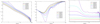 |
Fig. 1. Three-dimensional correlation and related functions of LCDM models for different particle density threshold δ0 limits. Left panel: CF. Central panel: gradient function, γ(r) = dlog g(r)/dlog r. Right panel: bias function, |
2.4. Calculation of projected CFs
In the distant observer approximation, we can use model data in rectangular spatial coordinates. In this approximation we calculated projected CFs from 2D density fields using the Szapudi et al. (2005) method. First we calculated 2D density fields on a 20482 grid by integrating the 3D field, δ(x, y, z), in the z-direction (by ignoring z-coordinates in the calculation of density fields in the selected z range):
We integrated cubic samples to get n sequentially located 2D sheets of size L0 × L0 × Lh−1 Mpc, where L = L0/n is the thickness of the sheets, and n = 1, 2, 4, …2048 is the number of sheets. It is clear that n = 1 corresponds to the whole sample in the z-direction of thickness, L = L0 = 512 h−1 Mpc, n = 2 corresponds to thickness 512/2 = 256 h−1 Mpc, and n = 2048 corresponds to thickness L = 512/2048 = 0.25 h−1 Mpc. For each n we calculated 2D CFs for all n sheets, and then found the mean CF and its error for a given n.
Examples of 2D density fields for various thickness L are given in Fig. 9 below. The upper panels of this figure show sheets of thickness L = 8 h−1 Mpc at various z locations and demonstrate the variance of the cosmic density field. The number of particles/galaxies in sheets is large, and errors are small; for some samples errors are shown in Fig. 6. In calculations, we used the mean density of the whole field for a given particle density limit ρ0 (absolute magnitude Mr limit). We also tested the case in which we used the mean density of each sheet separately for calibration. This increases CF errors, but has little influence on the amplitude of CFs.
Correlation functions were found using Lmax = 200 h−1 Mpc for 90 logarithmic distance bins. We label mean 2D sheets as LCDM.i, n and Mill.i, n, where i = ρ0 is the particle density limit used in the selection of particles for LCDM samples (absolute magnitude Mr limit for Millennium samples), and n is the number of sheets in the z-direction used to select particles (galaxies) for 2D samples. Millennium samples were analysed in real space and in redshift space. We denote these samples as Millr.i, n and Mills.i, n, respectively. Most of the analysis was made for Millennium samples in real space. For simplicity, we refer to these samples as Mill.i, n without the index r.
3. Comparison of spatial and projected correlation functions
In this section, we compare spatial CFs with respective projected functions. We focus on studying the influence of the thickness of 2D sheets on the behaviour of CFs. Also, we compare CFs in real and redshift space.
3.1. Three-dimensional correlation functions of LCDM models
LCDM model samples are based on all particles of the simulation and contain detailed information about the distribution of matter in regions of different density. As parameters, we use a particle density limit ρ0 in LCDM samples. For the argument in 3D CFs, we use the pair separation in 3D space,  . Three-dimensional CFs, gradient, and bias functions of LCDM models are shown in Fig. 1 for a set of particle density limits ρ0, as given in Table 1.
Three-dimensional CFs behave as expected. Samples with higher particle density limit, which correspond to brighter galaxies, have CFs with higher amplitudes. This is a well-known effect, and was detected by Bahcall & Soneira (1983) and Klypin & Kopylov (1983), and explained by Kaiser (1984) as the biasing phenomenon. The dependence of the correlation amplitude and the respective correlation length on galaxy luminosity has been the subject of many subsequent investigations. Among these studies, we mention here the work by Norberg et al. (2001), Zehavi et al. (2005, 2011), and related studies of the power spectra of galaxies based on recent large surveys such as Tegmark et al. (2002, 2004).
The mean shape of CFs is traditionally characterised by the slope of the CF, which is given in the last column of Table 1. For small particle density limits of ρ0 ≤ 5, the slope is close to the traditional value, γ ≈ −1.8, but for higher particle density limits the slope deepens. Here we see the influence of DM halos. A more detailed view of the shape of CFs is given by the gradient function, γ(r) = dlog g(r)/dlog r, presented in the central panel of Fig. 1. Here we clearly see two regimes of the CFs: on small scales, the CF describes the distribution of particles (galaxies) in halos (clusters); on large scales it describes the distribution of particles in the cosmic web. The presence of two regimes in CFs and their interpretation as the transition from clusters to filaments was first noticed by Zeldovich et al. (1982), and was discussed in detail by Einasto (1992). The presence of a minimum in the gradient function and its interpretation as the effective radius of halos of the cosmic web was noted by Zehavi et al. (2004). The outer radius of halos can be identified with the minimum of the gradient function near r ≈ 2 h−1 Mpc.
Dark matter halos of very different masses have almost identical DM profiles (Wang et al. 2020). As discussed by Einasto et al. (2020), at small separations the gradient function measures the mean profile of all DM halos. Near halo centres, the logarithmic gradient of DM halos is −1.5, and decreases to −3.0 at the periphery of halos (Wang et al. 2020). This explains the constant value of the gradient, γ(0.5) = − 1.5 at r = 0.5 h−1 Mpc, followed by a minimum near r ≈ 2 h−1 Mpc. For a small particle density limit of ρ0 < 5, small-mass DM halos dominate, and the minimum is not deep. With increasing particle density limit ρ0, low-density halos are excluded from the sample and more massive halos dominate. This leads to an increase in the depth of the minimum of γ(r). More massive halos have larger radii, thus the location of the minimum of the γ(r) function shifts to higher separation r values. It should be noted that a clear minimum is present only in LCDM models.
On larger scales, r ≥ 2 h−1 Mpc, the gradient function defines the fractal dimension of the sample, D(r) = 3 + γ(r). Our data show that the characteristic fractal dimension D(r) is a function of separation r. On very large scales, the fractal dimension approaches the value D(r) = 3 + γ(r)→3, which is characteristic of a random distribution of particles/galaxies.
The right panel of Fig. 1 shows the bias function for the LCDM samples, with various particle density limits ρ0. The limit ρ0 = 5 brings the percolation properties of the sample LCDM.05 close to the percolation properties of the faintest galaxies of the SDSS survey, Mr = −19.0; the limit ρ0 = 10 corresponds to L* galaxies of luminosity Mr = −20.5; see Einasto et al. (2019). For small particle density limits, ρ0 ≤ 2, lines of bias function b(r) are almost constant. In these samples, the smoothly distributed DM in low-density regions dominates the bias function. In models with higher particle density limits, ρ0 ≥ 5, at small separations, r ≤ 5 h−1 Mpc, the particle distribution in halos dominates the bias function. On larger separations, r ≥ 5 h−1 Mpc, bias functions are at an approximately constant level, and differ only by the amplitude A.
3.2. Three-dimensional correlation functions in real space in Millennium models
For Millennium samples, we used the Szapudi et al. (2005) method to calculated CFs and their derivates, gradient functions, γ(r), and relative bias function, bR(r). Functions were calculated for absolute magnitude limits Mr, as given in Table 2. In calculations with true model spatial positions x, y, z, we get functions in real space; see top panels of Fig. 2.
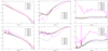 |
Fig. 2. Three-dimensional correlation and related functions of Millennium models. Top panels: real space. Bottom panels: redshift space. Left panels: CFs. Central panels: gradient functions. Right panels: relative bias functions. For comparison we show the 3D real space CF, the gradient, and the bias function of the sample Mill.17.4 with dashed lines in the bottom panels. As argument we use the pair separation in 3D real space. |
The slopes of the CFs in the Millennium samples are close to the conventional value, γ ≈ −1.8, for all magnitude Mr limits. LCDM samples behave differently and have higher negative slopes for samples with high ρ0 values. The reason for this difference is the weakness of clusters in Millennium samples. This difference between LCDM and Millennium samples is more pronounced in gradient functions γ(r). In Millennium samples, only the sample Mill.17.4 has a clear minimum around 2 h−1 Mpc; samples with higher luminosity limits have no minimum at this separation. The sample Mill.17.4 contains galaxies that are faint enough to populate clusters of galaxies with fainter members. Millennium samples with a higher luminosity limit contain less fainter cluster members, which makes the internal structure of the clusters less visible. In the samples with the highest luminosity limit, poor clusters disappear from the sample. In the remaining clusters only their main galaxies are visible, and therefore the correlation analysis considers these galaxies as isolated galaxies.
An important property of CFs is the dependence of their amplitude on particle density or luminosity limit Mr. The comparison of Figs. 1 and 2 shows that the dependence of CF amplitudes of Millennium galaxy samples on the luminosity limit is different from the dependence of LCDM CF amplitudes on the particle density limits. The amplitudes of the CFs of the LCDM samples increase approximately proportionally to the particle density limit of samples. In Millennium samples the amplitude A remains almost constant with increasing Mr up to Mr = −20.0. This dependence is shown in Fig. 3. A flat distribution of correlation radii with increasing luminosity has been found in galaxies by Einasto (1991), Norberg et al. (2001), Zehavi et al. (2005, 2011), and Einasto et al. (2019). This flat distribution of amplitudes of galaxy CFs can be explained by the absence of formation of very faint dwarf galaxies in voids. Dwarf galaxies form only as satellites in halos of brighter galaxies. This explains the almost constant amplitude of the CFs of galaxies of low luminosity, Mr > −20.0.
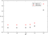 |
Fig. 3. Amplitudes A of the Millennium simulation CFs for various luminosity limits Mr. Real space and redshift space CF amplitudes are shown using black and red symbols, respectively. |
For Millennium galaxies, we calculated relative bias functions,  , where ξ(r) is the CF of the test sample, and ξ0(r) is the CF of the reference sample. In the top right panel of Fig. 2 we show relative bias functions of the Millennium model using CFs of Millennium samples of galaxies for various luminosity limits Mr in real space, and the CF of the sample Mill.17.4 in real space for reference. For Millennium samples, the CF of all DM is not available, and therefore it is possible to calculate only relative bias functions. Comparison of the right panels of Figs. 1 and 2 shows the difference.
3.3. Three-dimensional CFs in redshift space of Millennium models
We calculated CFs and gradient functions for Millennium samples in redshift space with galaxy positions in x, y unaffected, but as z positions we used redshift-distorted z coordinates, as seen by a distant observer. Redshift space CFs and related functions are shown in the bottom panels in Fig. 2.
The almost constant level of amplitude of CFs is valid both in real and redshift space; see Table 2 and Figs. 2 and 3. This property can be quantified by the amplitude correction factor of redshift CFs,

where As = ξ(6)s is the CF amplitude of a sample at 6 h−1 Mpc in redshift space, and Ar = ξ(6)r is the CF amplitude at 6 h−1 Mpc of the sample in real space. Amplitude correction factors C of Millennium galaxy samples in redshift space are given in Table 2. As we see, for fainter samples Mr > −20.0 the amplitude correction factor C is almost constant with the mean value C = 1.135 ± 0.001. This value is expected from the Kaiser (1987) effect — the contraction of superclusters in the vertical direction is, C2 = g, where g is calculated from Eq. (6) below.
The comparison of CFs shows that the amplitudes of Millennium samples in redshift space at small separations are much lower. This has a simple explanation: In redshift space, clusters of galaxies are expanded in the z-direction by velocity dispersions, and lose their compact character. This decreases the number of close pairs at small separations, and in this way decreases the amplitude of CFs. For this reason, CFs at small separations are shallower, and have a lower negative gradient γ(r); see Fig. 2. Galaxies from different clusters are partly mixed; this increases the scatter of the CF and its gradient function.
At large separations, the amplitudes of CFs in redshift space are larger. Here, the Kaiser (1987) effect is visible: in redshift space massive supercluster-type systems are contracted in the z-direction; their effective volume decreases, and the volume of voids between superclusters increases. This leads to the increase of the amplitude of CFs.
We calculated CFs in redshift space with FOG removed by compressing FOG to get equal dispersions of cluster galaxies in radial and tangential directions; a similar procedure was applied by Einasto et al. (1986) and Tegmark et al. (2004). The compression rate was found empirically without any assumptions regarding the underlying cosmology. Calculated CFs of the sample Mill.17.4 are shown in Fig. 4. The expected CF in redshift space can be found by multiplying the real space CF by a factor (Kaiser 1987):
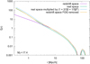 |
Fig. 4. Three-dimensional CFs of Mill.17.4 samples in real space, redshift space, Kaiser space, and redshift space with the FOG removed. |
where  , and b is the bias factor. We used Ωm = 0.25 (value used in Millennium simulation) and bias factor b = 1. Figure 4 shows that at r ≥ 5 h−1 Mpc, the CF in redshift space, expected from real space and using this conversion factor, coincides with the actual redshift space CF.
For comparison, we also calculated anisotropic two-point CFs for Millennium galaxies with magnitude limit Mr = −17.4 in redshift space, and in redshift space with FOG removed using the procedure described above; see Fig. 5. The right panel presents anisotropic 2D CF of Mill.17.4 galaxies in Kaiser space. As we see, FOGs are essentially removed; however some remnants are still visible. In spite of these remnants, the 3D CF of Mill.17.4 sample in redshift space with FOG removed coincides at small distances r ≤ 2 h−1 Mpc with the 3D CF in real space. At larger distances, it coincides with the 3D redshift CF; see Fig. 4.
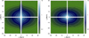 |
Fig. 5. Two-dimensional anisotropic CFs of Mill.17.4 samples in redshift space (left) and in redshift space with the FOG removed using the procedure described in the main text (right). |
The bottom right panel of Fig. 2 shows relative bias functions for Millennium galaxies in redshift space. Here we also use the sample Mill.17.4 in real space as reference. This function is determined by redshift distortions: On small scales, r ≤ 3 h−1 Mpc, the FOG effect dominates; on larger scales the contraction of superclusters by the Kaiser effect dominates.
The bottom left and right panels of Fig. 2 show that CFs and relative bias functions have peaks at r = 1 h−1 Mpc and elsewhere. To find the meaning of the peaks we made additional calculations of redshift space CFs using various resolutions in the Szapudi et al. (2005) method from Ngrid = 128 to Ngrid = 3072. These calculations showed that the effect is due to anisotropy and interference of redshift corrections on various scales, and each grid size generates peaks at different scales.
3.4. Two-dimensional correlation functions
We calculated 2D CFs, gradient functions, and relative bias functions for the LCDM and Millennium samples using the Szapudi et al. (2005) method, as described above. Results are shown in Fig. 6 for a series of sample thicknesses L = L0/nh−1 Mpc, using number of sheets n = 1, 2, 4, 8, 16, 32, 64, and 2048, which correspond to sheet thicknesses from the maximum, L = 512 h−1 Mpc (number of sheets n = 1), to the mean of n = 2048 most thin sheets, each of a thickness of L = 0.25 h−1 Mpc. We use LCDM.10 samples with particle density limit ρ0 = 10, and Millennium samples Mill.20.5 with luminosity limit Mr = −20.5. Both limits correspond approximately to L* galaxies (Einasto et al. 2019). As argument in 2D CFs we use the pair separation perpendicular to the line of sight for a distant observer,  .
.
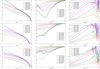 |
Fig. 6. Two-dimensional CFs and related functions for models for different thickness of 2D samples. Top row: LCDM model with particle density limit ρ0 = 10. Second row: Millennium samples with magnitude limit Mr = −20.5 in real space. Bottom row: Millennium samples with magnitude limit Mr = −20.5 in redshift space. Left panels: CFs. Central panels: gradient functions. Right panels: relative bias functions. As argument we use pair separations perpendicular to the line of sight, |

Two-dimensional CFs depend on two parameters, the thickness of the sheets, L = 512/nh−1 Mpc, and the particle density limit of LCDM samples, ρ0, or magnitude limit, Mr, of Millennium samples. The essential properties of the CFs are their amplitudes, A, and shape characteristics: slope γ, and gradient and relative bias functions. Correlation amplitudes of 2D samples of LCDM models are given in Table 3, and correlation amplitudes of 2D samples of Millennium models in real space are given in Table 4. Correlation amplitudes for full 2D samples LCDM.00 are printed in italics in the tables. For comparison, we provide the amplitudes of 3D CFs for various particle density limits in the last column, the amplitude of the 3D CF of the model LCDM.00 in boldface, that is, the full DM LCDM model. We calculated amplitudes of 2D Millennium samples also in redshift space; these are used in the bottom panels of Fig. 6.
Amplitudes of 2D CFs of LCDM models.
3.4.1. Two-dimensional correlation functions of LCDM model samples
The luminosity dependence of the 2D CFs of the LCDM model is similar to the luminosity dependence of 3D CFs. With increasing luminosity, the amplitude of CFs increases, as shown in Tables 1 and 2 for 3D functions, and in Tables 3 and 4 and Fig. 8 for 2D functions. This means that 2D density fields and respective CFs preserve the information on the luminosity dependence contained in 3D density fields and 3D CFs. To check this, we calculated the 2D CFs of the LCDM.00 model analytically, applying Eq. (A.5), and using the 3D CF of a LCDM halo model. The results of this calculation are shown in Fig. 7. As we see, the analytic model describes the decrease in amplitude of the 2D CFs with increasing sample thickness as well as the numerical integration by the Szapudi et al. (2005) method.
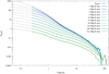 |
Fig. 7. Two-dimensional CFs of LCDM models, calculated from 2D density fields (solid coloured lines), and analytically from the 3D CF model using Eq. (A.5) (dashed lines). |
Amplitudes of 2D CFs of Millennium models.
The gradient function, γ(r), characterises the fine structure of the cosmic web. The top middle panel of Fig. 6 shows that the internal structure of the DM halos of the LCDM model is partially preserved in 2D CF gradient functions. As expected, this information is fully preserved in very thin 2D slices. The characteristic minimum of gradient functions near r ≈ 2 h−1 Mpc is visible, but has a lower amplitude. The mean gradient of LCDM 2D CFs at small separations, γ(r < 1) ≈ − 0.7, and varies in large limits, −1.7 ≤ γ(r) ≤ − 0.5 for separations 2 ≤ r ≤ 10 h−1 Mpc. The fine structure of DM halos is gradually erased with increasing thickness of 2D slices. At large separations, gradient functions approach zero values, as expected for random samples.
3.4.2. Two-dimensional correlation functions of Millennium model samples
The general shape of CFs is described by the slope γ of the CFs. The comparison of Figs. 1, 2 and 6 shows that 2D CFs are much shallower than 3D CFs. The slope of 2D CFs depends on the thickness of samples, L. This dependence is shown in the left panel of Fig. 8 for Millennium 2D samples in real space for various luminosity limits. For thick samples with L ≥ 32 h−1 Mpc, the slope is γ ≈ −0.9, close to the characteristic slope of 2D CFs, which is well known from early studies of CFs: Peebles (1973, 2001), and Peebles & Groth (1975). With decreasing thickness of 2D samples, the negative slope increases, and for very thin sheets reaches a value of γ ≈ −1.8, which is characteristic of 3D CFs. There is only a weak dependence of the slope on the magnitude limit, Mr.
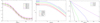 |
Fig. 8. Left panel: dependence of the slope γ of Millennium 2D CFs of various magnitude limits on the thickness of samples L. Middle panel: amplitudes A = ξ(6) of several LCDM and Millennium simulation 2D CFs as functions of the thickness of samples, L. For the Mill.17.4 sample, amplitudes are shown for real space and redshift space CFs. Short lines show 3D CF amplitudes of the same samples. The black dashed line shows the approximation A = 50/L. Right panel: fraction of zero-density cells (ρ ≤ 0.001) in 2D density fields, F0, as a function of the thickness of 2D samples, L. |
Figure 6 shows that the information on the internal structure of the clusters of the Millennium samples is fully lost in 2D CFs of simulated galaxies of the sample Mill.20.5 (and of samples with brighter luminosity limit). At this luminosity threshold, clusters contain only a few galaxies. In the 2D field, clusters are superposed by galaxies from different vertical locations in projection; see Fig. 9. The amplitudes of the 2D CFs of the Millennium samples are rather low (see Table 4), and in the calculation of the gradient function, the first constant term of the function g(r) = 1 + ξ(r) dominates. At small separations, the gradient function of the 2D Millennium CFs lies in the range −1.0 ≤ γ(r) ≤ − 0.2, depending on the thickness L. For thick samples over the whole separation interval the gradient functions have values of γ(r) > − 0.5, that is, the respective 2D CFs are similar to the CFs of samples with a random distribution of galaxies.
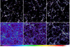 |
Fig. 9. Two-dimensional density fields of LCDM.10 models with particle density threshold ρ0 = 10. Top panels: 2D density fields of thickness L = 8 h−1 Mpc at z-coordinates 100, 200, 300. Bottom panels (from left to right): thickness L = 512, 128, 32 h−1 Mpc. We show the central sections of 2D density fields of size 256 × 256 h−1 Mpc. The colour scale is linear, and the code is identical in all panels. |
In the present context it is interesting that the difference between gradients of 2D and 3D CFs on small scales gradually fade away with decreasing thickness L of subsamples. The mean 2D CF of very thin slices is almost equal to the 3D CF of the same sample, as seen in Fig. 6 and in Tables 3 and 4. This is expected, because thin slices contain all essential spatial information of the 3D density field: the fraction of zero-density cells and the mutual distances of high-density regions. The last point is essential, as the CF is sensitive not to the location of galaxies/particles, but to their separations. Because of this property, the mean 2D CF of thin slices is equivalent to the 3D CF, in spite of the loss of information on the z-coordinates of galaxies/particles.
3.4.3. Amplitudes of 2D correlation functions
The middle panel of Fig. 8 shows the amplitudes of the 2D CFs from three LCDM simulations and one Millennium simulation as functions of the thickness of the samples, L. For the Mill.17.4 sample, amplitudes are shown for real and redshift space. Short horizontal lines on the left axis show amplitudes of 3D CFs of the same samples. At small thickness values, lines for 2D model samples smoothly approach the limits given by 3D samples. The figure shows that the decrease in the amplitude with increasing thickness is very regular, and almost identical in all samples relative to the amplitude of the 3D CF. A decrease in the amplitude of the 2D CF by about 10% is seen also at sheets of thickness L = 8 h−1 Mpc. At L = 512 h−1 Mpc, the amplitudes of 2D CFs are lower than the amplitudes of 3D CFs by more than an order of magnitude. Also, we see that the difference in amplitudes of Millennium samples in real and redshift space is very small.
The amplitudes shown in Fig. 8 were calculated numerically from 3D CFs using the Szapudi et al. (2005) method as described above. Integration using the analytical expression Eq. (A.5) yields identical results. As seen from Eq. (A.7), according to the Limber approximation, amplitudes are expected to be inversely proportional to thickness L. Figure 8 shows that the Limber approximation yields a good representation of the A(L) function for large thicknesses, L ≥ 30 h−1 Mpc.
The most essential aspect of Figs. 6 and 8 is their suggestion that the behaviour of the 2D CFs of samples of different thickness of LCDM and Millennium model samples is very similar: the amplitudes of 2D CFs depend significantly on sample thickness and are always lower than the amplitudes of the 3D CFs of the same sample. The greater the thickness of the 2D sample, the greater the difference between the amplitudes of 2D and 3D CFs. This behaviour is almost identical in all our samples, in LCDM and Millennium samples in real space, and in Millennium samples in redshift space. This similarity is remarkable, because test particles in samples are defined differently: DM particles with local density labels and simulated galaxies with luminosity labels. This similarity means that the geometrical properties of the cosmic web are very similar in both models, defined in our LCDM model by the particle density limits, ρ0, and in Millennium samples by the simulated galaxy luminosity limit, Mr. The similarity in the geometrical properties of the density fields, defined by LCDM models and SDSS galaxies, was demonstrated by Einasto et al. (2019) using the extended percolation analysis. Correlation and percolation analyses are sensitive to different aspects of the structure of the cosmic web, but yield similar results for the amplitude dependence on sheet thickness.
The second essential aspect of Fig. 8 is the shape of the A(L) function. At small thickness, L ≤ 10 h−1 Mpc, the amplitudes of 2D CFs are approximately equal to the amplitudes of 3D CFs. This means that the spatial structure of thin 2D slices is statistically similar to the spatial structure of the whole 3D web. Most importantly, the fraction of zero-density cells of the cosmic web is similar in thin 2D slices and in the whole 3D web. The fraction of zero-density cells, F0 (actually cells of density ρ ≤ 0.001), is shown in the right panel of Fig. 8, also as a function of 2D sheet thickness, L. We show the fraction F0 for four particle density limits, ρ0 = 1, 2, 5, 10. We see that, with increasing thickness, the fraction of zero-density cells in 2D slices decreases. The middle panel shows that, for thicknesses L ≥ 30 h−1 Mpc, the amplitude is inversely proportional to the thickness, A ∝ 1/L. In this thickness range, the decrease in the fraction of zero-density cells F0 with increasing thickness L of 2D slices is the deciding factor that determines the amplitude of 2D CFs. We discuss this aspect further in the following section.
3.4.4. Relative bias functions of 2D CFs
The right panels of Fig. 6 show relative bias functions calculated for particle density limit ρ0 = 10 for the LCDM model, and magnitude limit Mr = −20.5 for Millennium galaxy samples. In calculations of relative bias functions we used the samples LCDM.10 and Mill.20.5 (in real space) as reference samples for the 3D CFs. We show the dependence of relative bias functions on sample thickness L = 512/nh−1 Mpc, where n = 1, 2, 4, 8, 16, 32, 62, 2048 is the number of sheets in 2D density fields.
Relative bias functions show the dependence of relative CFs on the separation r. Amplitudes A were calculated for a fixed separation value, r = 6 h−1 Mpc. The figure shows that the decrease in the bias function and amplitude with increasing sample thickness L is regular, and similar in LCDM and Millennium samples in real space. All relative bias functions have values of less than unity, that is, 2D CFs have lower amplitudes than 3D CFs. One exception is the relative bias function of the Millennium samples in redshift space, shown in the bottom right panel of Fig 3.3. For thinner samples, n ≥ 8, we see relative bias values of bR ≥ 1, which is caused by redshift distortions due to the Kaiser effect. This excess is seen also in CFs shown in the bottom left panel.
4. Correlation functions as descriptors of the cosmic web
Here, we describe spatial and projected density fields first, and their description by CFs. Thereafter, we analyse CFs as descriptors of the cosmic web. Finally, we describe some earlier work on the determination of CFs and power spectra of galaxies, and discuss the problem of whether 3D CFs can be calculated from 2D CFs.
4.1. Spatial and projected density fields
The essential feature of the cosmic web is its spatial structure or pattern. The spatial CF characterises the geometrical properties of the cosmic web in a general and global way. To understand the influence of the pattern of the cosmic web on properties of CFs, let us look at the geometry of the density field of the cosmic web, as given by 2D and 3D data.
Figure 9 shows 2D density fields of the model LCDM.10 using particle density limit ρ0 = 10, and at various thicknesses. The upper panels present 2D density fields of thin slices of thickness L = 8 h−1 Mpc in x, y coordinates at three z locations. The thickness of the 2D density field in the bottom left panel is L = 512 h−1 Mpc, that is, the whole cube of our LCDM.10 model. In the bottom middle and bottom right panels, the thicknesses are L = 128 h−1 Mpc and L = 32 h−1 Mpc, respectively. In the calculation of the 2D density fields we used the 3D density field with a resolution of 512 × 512; in the figure we show only the central 256 × 256 h−1 Mpc sections of the fields. Galaxies can form in regions where the local density is high enough; a particle density limit of ρ0 = 10 corresponds approximately to L* galaxies of SDSS magnitude Mr − 5 log h = −20.5 using the percolation test; see Fig. 10 by Einasto et al. (2019). Thus, in Fig. 9 all DM particles in low-density regions and DM particles corresponding to faint galaxies, Mr > −20.5, are excluded. In this way, Fig. 9 imitates the 2D distribution of matter in real galaxies in samples of different thickness.
Two-dimensional density fields in the top panels of Fig. 9 are so thin that their morphological properties are close to those of the 3D density field of the same model, namely the fraction of high- and low-density regions and mutual distances between high-density regions. However, as seen from Table 3, the mean amplitude of CFs of stacked 2D LCDM.10.0064 model sheets of thickness 8 h−1 Mpc differs slightly from the amplitude of the 2D model LCDM.10.2048, which is approximately equivalent to the 3D model LCDM.10; compare Tables 1 and 3. This means that at a thickness L = 8 h−1 Mpc, the 3D features of the web are already partly smoothed out in the 2D field.
Essential elements of the cosmic web are high-density regions (clusters and filaments) and voids, which together form the pattern of the web. The detailed structure of the web is seen in the top panels of Fig. 9. High-density regions are surrounded by zero-density voids, occupying most of the volume of the density field. The fraction of cells with zero-density in 2D density fields of thickness 8 h−1 Mpc is F0 = 0.80; see Fig. 8, and the filling factor of voids in the LCDM 3D density field is FV = 0.86; see Table 1 of Einasto et al. (2018). There are faint filaments of DM in voids, but the density is too low to start galaxy formation, and therefore the density field of galaxies has zero density there. The characteristic scale of halos containing galaxies is a few h−1 Mpc; small visible regions in Fig. 9 have approximately this diameter. Clusters and filaments in sheets at different z locations are located in various x, y-positions; compare different top panels of Fig. 9.
Correlation functions are sensitive to particle/galaxy separations, not locations. For this reason, the statistical properties of the 2D CFs of very thin sheets at various z-locations are similar, and close to statistical properties of 3D correlation functions. This statistical similarity can be seen in the mean CF of n = 2048 thin sheets of thickness L = 512/n = 0.25 h−1 Mpc, and is shown in Fig. 6 together with the 3D CF of the same particle density limit ρ0.
With increasing thickness L of 2D density fields, the fraction of cells with zero density rapidly decreases. This is clearly seen in Fig. 9 visually, and in Fig. 8 graphically. The fraction of zero-density cells is F0 = 0.53, 0.13, 5.4 × 10⁻⁴ for thicknesses L = 32, 128, 512 h−1 Mpc of the 2D density field of the model LCDM.10. For models LCDM.05 and LCDM.02, there are already no zero-density cells at thicknesses L = 512 and L = 256 h−1 Mpc, respectively; see right panel of Fig. 8.
4.2. Correlation function amplitude as a cosmological parameter
Amplitudes of CFs depend on many factors: (i) cosmological parameters: matter-energy densities Ωb, Ωm, ΩΛ, and the present rms matter fluctuation amplitude averaged over a sphere of radius 8 h−1 Mpc, σ8; (ii) luminosities of galaxies; (iii) systematic motions of galaxies in clusters – the FOG effect, and the flow of galaxies toward attractors – the Kaiser effect. Systematic motions decrease the amplitudes of 3D CFs on small scales and increase them on large scales. The increase of CF amplitudes on large scales is well described by the dynamical model by Kaiser (1987).
The present analysis shows that amplitudes of 2D CFs are influenced by an additional factor: the thickness of samples, L. The dependence of the amplitudes of 2D CFs on sample thickness follows from the spatial properties of the cosmic web. The cosmic web consists of galaxies located in an intertwined filamentary pattern, and leaving most of the space void of galaxies. In projection, clusters and filaments fill in voids, depending on the thickness of samples. For this reason, 2D and 3D patterns of the web are qualitatively different. The thicker the 2D sheets, the greater the difference.
The filling factor of high-density regions of the model LCDM.05 is 0.10; the SDSS sample has a similar filling factor with absolute magnitude limit Mr = −19.0; see Einasto et al. (2019). The rest of the volume, that is, 90%, has zero density. This means that 3D density fields corresponding to galaxies as well as thin slices of the 2D density field are dominated by zero-density cells. In stacked thick 2D sheets, clusters and filaments at various z are projected to the 2D x, y plane at different positions, and in this way fill in voids in the 2D density field. This is clearly seen in the bottom panels of Fig. 9.
The correlation functions of our models were calculated using density fields applying the method by Szapudi et al. (2005). The power spectrum of our LCDM model was calculated by Einasto et al. (2019). As input for both correlation and power spectrum analysis, we use the density contrast field,  , used for power spectrum analysis as follows:
where k is the wavenumber, δ = ρ − 1 is the density contrast, and ρ is the density in mean density units. The density field used to find power spectra or CFs can be divided into four main regions: zero-density regions with ρ = 0 and δ = −1, low-density regions with 0 ≤ ρ ≤ 2 and |δ|≤1, medium-density regions with 2 ≤ ρ ≤ 10, and high-density regions with ρ > 10. Both the power spectrum and the CF depend on fractions of different density regions. In the full DM model, all basic regions are present. Over most of the volume, the density is less than the mean density, or exceeds the mean density only slightly, ρ ≤ 2. In these low-density regions, density contrast lies in the interval −1 ≤ δ ≤ 1, and has a mean value of |δ|≈0.5 or less. Here, matter remains in diffuse form, galaxy formation is impossible, and the density field of galaxies has zero density, ρ = 0, δ = −1, and |δ|=1. All cells of the DM density field, which had density contrast in the interval −1 ≥ δ ≥ 1, have a value |δ|=1 in the galaxy density field. The power spectrum (and CF) is a sum over all density contrasts. The greater the fraction of cells with zero density, the higher the amplitude of power spectra and CFs. When we consider density fields of increasing luminosity (particle density) limit, with increasing luminosity limit, we see an increasing fraction of medium density cells, which previously had densities in the interval 2 ≤ ρ ≤ 10, move to zero-density cells with |δ|=1, which leads to a further increase in the amplitude of the power spectra and CFs.
This analysis shows that amplitudes of CFs and power spectra depend essentially on the fraction of cells of the density field with zero density. This is the reason why the amplitudes of the CFs and power spectra of galaxies are higher than the amplitudes of the CFs and power spectra of DM, and also why the amplitudes of CFs and power spectra of luminous galaxies are higher than the amplitudes of CFs and power spectra of fainter galaxies.
The same argument is valid in the comparison of 2D and 3D density fields. The essential difference between 2D and 3D density fields is in the fraction of zero-density regions. In 2D density fields, high-density regions from various distances overlap and fill in voids. The thicker the 2D density fields, the fewer zero-density cells they contain. We conclude that the essential difference between 2D and 3D (and thin 2D) density fields is the near absence of visible zero-density regions in thick 2D fields. To summarise the comparison of 2D and 3D density fields, we can say that the large fraction of zero-density regions of 3D fields, wiped out in various amounts in 2D fields, decreases the amplitude of 2D CFs; this effect increases with increasing thickness of the 2D field. For this reason, the amplitudes of power spectra and CFs for stacked 2D density fields are lower than the amplitudes of power spectra and 3D CFs based on 3D density fields. For the same reason, the amplitudes of the power spectra and 3D CFs of galaxies are greater than the amplitudes of 3D CFs of DM.
The similarity between the 2D CFs of Millennium simulation galaxies and the 2D CFs of LCDM samples shows that the influence of zero-density regions in both models is similar, also for Millennium models in redshift space. An analytical description of the relation between 2D and 3D two-point correlators is given in the appendix.
4.3. Comparison with earlier work
In classical correlation studies, the first step was to find the estimate of the anisotropic 3D CF by counting pairs DD(rp, π) (Davis & Peebles 1983). The next step was the calculation of the 2D CF using Eq. (B.1). As a final step Davis & Peebles (1983) calculated the 3D CF using the inversion according to Eq. (B.2), with smoothed w(r⊥) 2D CF.
Norberg et al. (2001) selected galaxies in conical shells of various thicknesses from rmax − rmin ≈ 25 h−1 Mpc for the faintest galaxies (Mb − 5 log h ≈ −18) to rmax − rmin ≈ 700 h−1 Mpc for the most luminous subsamples. Zehavi et al. (2005, 2011) investigated projected CFs of SDSS galaxies of different luminosity. Authors applied standard practice by Davis & Peebles (1983) and computed projected CFs using Eq. (B.1), and real-space correlation functions using Eq. (B.2). Samples of various absolute magnitude bins were located in spherical shells of various thicknesses.
A correlation analysis of SDSS samples using 3D CFs in redshift space was performed by Hawkins et al. (2003) and Einasto et al. (2020). These analyses showed that correlation radii from 3D analysis in redshift space are about a factor 1.35 higher than from the 2D analysis by Zehavi et al. (2011). This difference is probably due to projection effects in the 2D analysis.
Shi et al. (2016, 2018) elaborated a method to calculate real-space two-point CFs of galaxies from redshift data. The method consists of several steps: calculating the mass-density field from the luminosity density field, reconstructing the velocity field on quasi-linear scale, and correction for the Kaiser and FOG effects. The method was checked using mock galaxy catalogues based on a simulation of 30723 particles in a box of 500 h−1 Mpc side-length. Two-point spatial CFs of mock catalogues in true real space, redshift space, Kaiser space, and FOG space are relatively similar to the corresponding CFs in our study, shown in Figs. 1 and 4.
4.4. The information content of 2D CFs
Our previous analysis showed that calculation of projected CFs from spatial CFs influences the information content of CFs. We now try to estimate the change of information content in all steps of the standard procedures by Davis & Peebles (1983). The anisotropic CF, ξ3D(r∥, r⊥), found by counting pairs of separations of galaxies, has the maximal information content possible from observational data in terms of angular positions and redshifts of galaxies. Observational data are influenced by redshift distortions. To avoid distortions, the ξ3D(r∥, r⊥) is integrated along the line of sight (see Eq. (4) or Eq. (B.1)), to get 2D CFs. Our analysis shows that this operation preserves information on the luminosity dependence of the CF, which is confirmed by comparison of correlation radii of galaxies of various luminosity obtained by Davis & Peebles (1983), Norberg et al. (2001), and Zehavi et al. (2005, 2011), with the results of authors using different methods (Hawkins et al. 2003).
Our study also shows that integration according to Eq. (A.4) yields 2D CFs with decreasing amplitudes, depending on the thickness of the sheets. This means that, because of projection effects, information on zero-density regions in the 3D density field is partly lost, as demonstrated graphically in Fig. 9, and numerically in Figs. 6 and 8. In real observational samples, spherical coordinates are used and integration is done according to Eq. (B.1). The projection effect to 2D CFs is smaller than expected from Table 4, because observed galaxy samples are conical, and nearby regions in conical shells have a smaller input than more distant ones. Thus, the decrease in the amplitude of 2D CFs is not well determined and depends on the sample used.
We also find that in 2D density fields, the information on the internal structure of clusters of galaxies is lost, especially in redshifts space; see the behaviour of gradient functions in Fig. 6. This explains the observational result by Maddox et al. (1990) that the angular CF of the Automatic Plate Measuring (APM) survey of galaxies has a constant slope, γ ≈ −0.7, over a wide range of angular scales and galaxy apparent magnitudes. As information on the internal structure of clusters is lost, this result can be explained as evidence for a mean constant fractal dimension of the spatial distribution of galaxies of the survey.
Three-dimensional density fields contain more information than 2D density fields, and therefore inversion to get 3D CFs from 2D CFs (Eq. (B.2)) adds information. The relation between projected and spatial CFs is similar to the relation between the projected and spatial densities of galaxies, which are used to calculate their dynamical models, starting from Wyse & Mayall (1942) and Kuzmin (1952). The information gain comes in this case from the assumption that galaxies are spatial ellipsoids of rotation, which was specifically noted by Kuzmin (1952). The information gain in the calculation of 3D CFs from 2D CFs using Eq. (B.2) comes from the tacit assumption that the spatial and projected structures of the cosmic web are statistically similar, which is not the case. The difference between 2D and 3D data can be treated in information terms: information on zero-density regions is lost in 2D density fields and in respective 2D CFs. This information loss is characterised by decreasing amplitudes of 2D CFs. When 2D CFs are used to calculate 3D CFs, this information on 3D density fields is not restored, and therefore amplitudes of 3D CFs found by inversion (see Eq. (B.2)) are still based on amplitudes of 2D CFs distorted by projection effects. In other words, it is impossible to calculate 3D density fields, which are close to sheets in the top panels of Fig. 9 using 2D density fields, as shown in the lower panels.
5. Conclusions
In this paper, we analyse the relationship between projected and spatial CFs. To avoid complications related to observational selection effects we studied the relationship using simulated DM models, using our own LCDM model and the Millennium simulation. Both simulations were made in a box of size ∼500 h−1 Mpc. To study spatial distributions of model objects we used DM particles in our model and simulated galaxies in the Millennium model.
We calculated CFs with the Szapudi et al. (2005) method, which allows us to consider CFs as descriptors of the density field of the cosmic web. We calculated 3D CFs for both models, for the Millennium model in real and redshift space. We found projected 2D CFs in the distant observer approximation in the z-direction. In addition to CFs, we used gradient functions, γ(r) = = dlog g(r)/dlog r, where g(r) = 1 + ξ(r), and relative bias functions,  , where ξC(r, ρ0) is the CF of clustered matter (galaxies), and ξr(r) is the CF of the reference sample. Additionally, we quantify CFs by their amplitudes at separation 6 h−1 Mpc, A = ξ(6).
The general results of our study can be summarised as follows.
-
The dominant elements of the cosmic web are clusters and filaments, which are separated by voids filling most of the volume. Clusters and filaments are located at different positions in 2D sheets. As a result, in projection, clusters and filaments fill in 2D voids, which leads to a decrease in the amplitudes of the CFs (and power spectra). For this reason, the amplitudes of 2D CFs are lower than the amplitudes of 3D CFs, and the thicker the 2D sample, the greater the difference.
-
In 2D CFs, information on the luminosity dependence is preserved, information on the internal structure of clusters is lost, and information on the amplitudes of CFs is partially lost, depending on the thickness of the sample.
The amplitude of CFs (and power spectra) is an important cosmological parameter which depends on many factors – cosmological parameters, systematic motions of galaxies, luminosities of galaxies, and thickness of 2D samples. Luminosities and thickness influence 2D CFs in oposite directions: increasing luminosity increases, but increasing thickness decreases CF amplitudes.
Acknowledgments
Our special thanks are to Enn Saar for many discussions, and to anonymous referees for stimulating suggestions that greatly improved the paper. We thank the Millennium team for making results of their simulations public. This work was supported by institutional research funding IUT26-2 and IUT40-2 of the Estonian Ministry of Education and Research, and by the Estonian Research Council grants PRG803, PRG1006 and MOBTT5. We acknowledge the support by the Centre of Excellence “Dark side of the Universe” (TK133) financed by the European Union through the European Regional Development Fund.
References
- Bahcall, N. A., & Soneira, R. M. 1983, ApJ, 270, 20 [Google Scholar]
- Bahcall, N. A., Ostriker, J. P., Perlmutter, S., & Steinhardt, P. J. 1999, Science, 284, 1481 [Google Scholar]
- Bertschinger, E. 1995, ArXiv e-prints [arXiv:astro-ph/9506070] [Google Scholar]
- Coles, P., & Chiang, L.-Y. 2000, Nature, 406, 376 [NASA ADS] [CrossRef] [PubMed] [Google Scholar]
- Croton, D. J., Springel, V., White, S. D. M., et al. 2006, MNRAS, 365, 11 [NASA ADS] [CrossRef] [Google Scholar]
- Davis, M., & Peebles, P. J. E. 1983, ApJ, 267, 465 [NASA ADS] [CrossRef] [Google Scholar]
- Einasto, M. 1991, MNRAS, 252, 261 [NASA ADS] [CrossRef] [Google Scholar]
- Einasto, M. 1992, MNRAS, 258, 571 [Google Scholar]
- Einasto, J., Saar, E., & Klypin, A. A. 1986, MNRAS, 219, 457 [Google Scholar]
- Einasto, J., Suhhonenko, I., Liivamägi, L. J., & Einasto, M. 2018, A&A, 616, A141 [Google Scholar]
- Einasto, J., Liivamägi, L. J., Suhhonenko, I., & Einasto, M. 2019, A&A, 630, A62 [Google Scholar]
- Einasto, J., Hütsi, G., Kuutma, T., & Einasto, M. 2020, A&A, 640, A47 [Google Scholar]
- Einasto, J., Klypin, A., Hütsi, G., Liivamägi, L. J., & Einasto, M. 2021, A&A, 652, A94 [Google Scholar]
- Hawkins, E., Maddox, S., Cole, S., et al. 2003, MNRAS, 346, 78 [Google Scholar]
- Jackson, J. C. 1972, MNRAS, 156, 1 [Google Scholar]
- Kaiser, N. 1984, ApJ, 284, L9 [Google Scholar]
- Kaiser, N. 1987, MNRAS, 227, 1 [Google Scholar]
- Klypin, A. A., & Kopylov, A. I. 1983, Sov. Astron. Lett., 9, 41 [NASA ADS] [Google Scholar]
- Kuzmin, G. G. 1952, Publ. Tartu Astrofizica Obs., 32, 211 [Google Scholar]
- Maddox, S. J., Efstathiou, G., Sutherland, W. J., & Loveday, J. 1990, MNRAS, 242, 43 [Google Scholar]
- Moore, A. W., Connolly, A. J., Genovese, C., et al. 2001, in Mining the Sky, eds. A. J. Banday, S. Zaroubi, & M. Bartelmann, 71 [Google Scholar]
- Norberg, P., Baugh, C. M., Hawkins, E., et al. 2001, MNRAS, 328, 64 [Google Scholar]
- Pandey, B., White, S. D. M., Springel, V., & Angulo, R. E. 2013, MNRAS, 435, 2968 [CrossRef] [Google Scholar]
- Peebles, P. J. E. 1973, ApJ, 185, 413 [NASA ADS] [CrossRef] [Google Scholar]
- Peebles, P. J. E. 1980, The Large-scale Structure of the Universe, Princeton Series in Physics (Prinseton: Prinseton University Press) [Google Scholar]
- Peebles, P. J. E. 2001, in Historical Development of Modern Cosmology, eds. V. J. Martínez, V. Trimble, & M. J. Pons-Bordería, ASP Conf. Ser., 252, 201 [Google Scholar]
- Peebles, P. J. E., & Groth, E. J. 1975, ApJ, 196, 1 [Google Scholar]
- Repp, A., & Szapudi, I. 2019a, ArXiv e-prints [arXiv:1904.05048] [Google Scholar]
- Repp, A., & Szapudi, I. 2019b, MNRAS, submitted [arXiv:1912.05557] [Google Scholar]
- Sargent, W. L. W., & Turner, E. L. 1977, ApJ, 212, L3 [Google Scholar]
- Shi, F., Yang, X., Wang, H., et al. 2016, ApJ, 833, 241 [Google Scholar]
- Shi, F., Yang, X., Wang, H., et al. 2018, ApJ, 861, 137 [Google Scholar]
- Springel, V. 2005, MNRAS, 364, 1105 [Google Scholar]
- Springel, V., White, S. D. M., Jenkins, A., et al. 2005, Nature, 435, 629 [NASA ADS] [CrossRef] [PubMed] [Google Scholar]
- Stauffer, D. 1979, Phys. Rep., 54, 1 [Google Scholar]
- Szapudi, I., Prunet, S., Pogosyan, D., Szalay, A. S., & Bond, J. R. 2001, ApJ, 548, L115 [Google Scholar]
- Szapudi, I., Pan, J., Prunet, S., & Budavári, T. 2005, ApJ, 631, L1 [Google Scholar]
- Tegmark, M., Hamilton, A. J. S., & Xu, Y. 2002, MNRAS, 335, 887 [Google Scholar]
- Tegmark, M., Blanton, M. R., Strauss, M. A., et al. 2004, ApJ, 606, 702 [NASA ADS] [CrossRef] [Google Scholar]
- Tully, R. B., & Fisher, J. R. 1978, in Large Scale Structures in the Universe, eds. M. S. Longair, & J. Einasto, 79, 31 [Google Scholar]
- Wang, J., Bose, S., Frenk, C. S., et al. 2020, Nature, 585, 39 [Google Scholar]
- Wyse, A. B., & Mayall, N. U. 1942, ApJ, 95, 24 [Google Scholar]
- Zehavi, I., Weinberg, D. H., Zheng, Z., et al. 2004, ApJ, 608, 16 [Google Scholar]
- Zehavi, I., Zheng, Z., Weinberg, D. H., et al. 2005, ApJ, 630, 1 [Google Scholar]
- Zehavi, I., Zheng, Z., Weinberg, D. H., et al. 2011, ApJ, 736, 59 [NASA ADS] [CrossRef] [Google Scholar]
- Zeldovich, Y. B., Einasto, J., & Shandarin, S. F. 1982, Nature, 300, 407 [NASA ADS] [CrossRef] [Google Scholar]
Appendix A: Two-point function of the projected field
Here we briefly describe the relation between 2D and 3D two-point correlators. In the following we assume a sufficiently small survey volume such that evolutionary and lightcone effects can be neglected. We assume the validity of the cosmological principle, that is, statistical homogeneity and isotropy of the cosmic density field. Additionally, we do not include redshift-space distortions, because we focus on real-space two-point functions.
The density contrast is defined as is customary:
where n(r) is the comoving number density of tracer objects at spatial location r and  is the corresponding average density.
In the following we consider plane-parallel and spherical projections of the 3D field separately.
A.1. Plane-parallel geometry
Assuming appropriately normalized projection and selection function w(r), namely
the projected 2D overdensity field can be expressed as
The two-point correlation function of the projected density field can now be obtained. According to the cosmological principle we can always choose one point to be at the origin, that is, r⊥,1 = 0, and for the other we assume r⊥,2 = R with modulus R ≡ |R|. Thus, one can write
In the case of a uniform selection within the range [0, L], that is, w(r) = 1/L, the above result can be expressed as
In Eq. (A.4) the ξ3D part of the integrand is peaked around r1 = r2. If the selection function varies smoothly in comparison, it can be pulled out of the second integral (this is the essence of the Limber approximation, e.g., Peebles (1980)), giving
where we have introduced new dummy variables r1 → r and r2 − r1 → x. In the case of a uniform selection within the range [0, L], the above result can be expressed as

A.2. Spherical geometry
The above results can be extended for the case of spherical geometry. Here the results have the simplest form once the radial selection and projection function is normalized as
In that case the analogue of Eq. (A.4) reads

where  with
with  ,
, the radial unit vectors marking the two points.
The case with uniform selection in the range [D − L/2, D + L/2], that is, the analogue of Eq. (A.5), can be written as

In the case of slowly varying selection and with small-angle approximation, Eq. (A.9) can be recast as follows (this is a standard Limber’s formula):
where new dummy variables r1 → r and r2 − r1 → x were introduced.
Appendix B: Projected two-point function
Very often, in order to avoid complications caused by redshift-space distortions, the spatial two-point CF which is evaluated as a 2D function of radial and transverse separations, is integrated along the radial direction, resulting in the following quantity:
The above has a form of the Abel integral equation, which is often inverted to recover the real-space correlation function. The analytic form for the inversion is given by the following relation

However, in the presence of measurement errors this inversion is not a well posed problem (note that it involves taking derivatives from the noisy data), and thus needs additional assumptions for regularisation purposes (often one assumes a specific functional form for ξ3D, for example a simple power law). In addition, instead of using all available information, which would demand somewhat more complicated modelling in order to also capture the signal stored in the redshift-space distortions, the line-of-sight integration results in a generic signal loss.
It is instructive to note that the above result Eq. (B.1) is almost identical to Eq. (A.7). This is only so under the validity of the Limber approximation, that is, in the case where the projection and correlator calculation operations effectively commute. In general, there is a clear difference between the projected CF and the CF of the projected field.
All Tables
All Figures
|
Fig. 1. Three-dimensional correlation and related functions of LCDM models for different particle density threshold δ0 limits. Left panel: CF. Central panel: gradient function, γ(r) = dlog g(r)/dlog r. Right panel: bias function, |
| In the text | |
|
Fig. 2. Three-dimensional correlation and related functions of Millennium models. Top panels: real space. Bottom panels: redshift space. Left panels: CFs. Central panels: gradient functions. Right panels: relative bias functions. For comparison we show the 3D real space CF, the gradient, and the bias function of the sample Mill.17.4 with dashed lines in the bottom panels. As argument we use the pair separation in 3D real space. |
| In the text | |
|
Fig. 3. Amplitudes A of the Millennium simulation CFs for various luminosity limits Mr. Real space and redshift space CF amplitudes are shown using black and red symbols, respectively. |
| In the text | |
|
Fig. 4. Three-dimensional CFs of Mill.17.4 samples in real space, redshift space, Kaiser space, and redshift space with the FOG removed. |
| In the text | |
|
Fig. 5. Two-dimensional anisotropic CFs of Mill.17.4 samples in redshift space (left) and in redshift space with the FOG removed using the procedure described in the main text (right). |
| In the text | |
|
Fig. 6. Two-dimensional CFs and related functions for models for different thickness of 2D samples. Top row: LCDM model with particle density limit ρ0 = 10. Second row: Millennium samples with magnitude limit Mr = −20.5 in real space. Bottom row: Millennium samples with magnitude limit Mr = −20.5 in redshift space. Left panels: CFs. Central panels: gradient functions. Right panels: relative bias functions. As argument we use pair separations perpendicular to the line of sight, |
| In the text | |
|
Fig. 7. Two-dimensional CFs of LCDM models, calculated from 2D density fields (solid coloured lines), and analytically from the 3D CF model using Eq. (A.5) (dashed lines). |
| In the text | |
|
Fig. 8. Left panel: dependence of the slope γ of Millennium 2D CFs of various magnitude limits on the thickness of samples L. Middle panel: amplitudes A = ξ(6) of several LCDM and Millennium simulation 2D CFs as functions of the thickness of samples, L. For the Mill.17.4 sample, amplitudes are shown for real space and redshift space CFs. Short lines show 3D CF amplitudes of the same samples. The black dashed line shows the approximation A = 50/L. Right panel: fraction of zero-density cells (ρ ≤ 0.001) in 2D density fields, F0, as a function of the thickness of 2D samples, L. |
| In the text | |
|
Fig. 9. Two-dimensional density fields of LCDM.10 models with particle density threshold ρ0 = 10. Top panels: 2D density fields of thickness L = 8 h−1 Mpc at z-coordinates 100, 200, 300. Bottom panels (from left to right): thickness L = 512, 128, 32 h−1 Mpc. We show the central sections of 2D density fields of size 256 × 256 h−1 Mpc. The colour scale is linear, and the code is identical in all panels. |
| In the text | |
Current usage metrics show cumulative count of Article Views (full-text article views including HTML views, PDF and ePub downloads, according to the available data) and Abstracts Views on Vision4Press platform.
Data correspond to usage on the plateform after 2015. The current usage metrics is available 48-96 hours after online publication and is updated daily on week days.
Initial download of the metrics may take a while.