| Issue |
A&A
Volume 651, July 2021
|
|
|---|---|---|
| Article Number | L8 | |
| Number of page(s) | 5 | |
| Section | Letters to the Editor | |
| DOI | https://doi.org/10.1051/0004-6361/202140895 | |
| Published online | 16 July 2021 | |
Letter to the Editor
Redshift evolution of the Amati relation: Calibrated results from the Hubble diagram of quasars at high redshifts
1
Department of Astronomy, Beijing Normal University, Beijing 100875, PR China
e-mail: This email address is being protected from spambots. You need JavaScript enabled to view it.
, This email address is being protected from spambots. You need JavaScript enabled to view it.
, This email address is being protected from spambots. You need JavaScript enabled to view it.
2
Beijing Planetarium, Beijing 100044, PR China
3
School of Electrical and Electronic Engineering, Wuhan Polytechnic University, Wuhan 430023, PR China
Received:
26
March
2021
Accepted:
22
June
2021
Abstract
Gamma-ray bursts (GRBs) have long been proposed as a complementary probe to type Ia supernovae (SNe Ia) and the cosmic microwave background to explore the expansion history of the high-redshift universe, mainly because they are bright enough to be detected at greater distances. Although they lack definite physical explanations, many empirical correlations between GRB isotropic energy or luminosity and some directly detectable spectral or temporal properties have been proposed to make GRBs standard candles. Since the observed GRB rate falls off rapidly at low redshifts, this thus prevents a cosmology independent calibration of these correlations. In order to avoid the circularity problem, SN Ia data are usually used to calibrate the luminosity relations of GRBs in the low redshift region (limited by the redshift range for SN Ia sample), and then they are extrapolate the luminosity relations to the high redshift region. This approach is based on the assumption of no redshift evolution for GRB luminosity relations. In this work, we suggest the use of a complete quasar sample in the redshift range of 0.5 < z < 5.5 to test such an assumption. We divided the quasar sample into several subsamples with different redshift bins, and used each subsample to calibrate the isotropic γ-ray equivalent energy of GRBs in relevant redshift bins. By fitting the newly calibrated data, we find strong evidence that the most commonly used Amati relation between spectral peak energy and isotropic-equivalent radiated energy shows no, or marginal, evolution with redshift. Indeed, at different redshifts, the coefficients in the Amati relation could have a maximum variation of 0.93% at different redshifts, and there could be no coincidence in the range of 1σ.
Key words: gravitational waves / stars: neutron / stars: oscillations / quasars: general
© ESO 2021
1. Introduction
As the most intense explosions in the universe, gamma-ray bursts (GRBs) are bright enough to be detected in the high-redshift range up to at least z ∼ 10 (Tanvir et al. 2009; Salvaterra et al. 2009), so that GRBs have been widely discussed as a complementary probe to type Ia supernovae (SNe Ia) and the cosmic microwave background (CMB) to explore the expansion history of the high-redshift universe (Amati & Della 2013; Wang et al. 2015, for a review). In order to make GRBs standard candles, many empirical correlations between their isotropic energy or luminosity and some directly detectable spectral or temporal properties have been proposed. For instance, Amati et al. (2002) discovered a correlation between the isotropic bolometric emission energy (Eiso) and the rest-frame peak energy (Ep, z), later Ghirlanda et al. (2004a) proposed that there exists an even tighter correlation between Ep, z and the beaming-corrected bolometric emission energy (Eγ). In order to reduce the scatter of the correlations, several multiple relations have also been proposed, such as the Eiso – Ep, z – tb, z relation (Liang & Zhang 2005), among others (see more correlations reviewed in Ghirlanda et al. 2004b; Demianski et al. 2017a; Zhang 2018).
These GRB luminosity indicators have been widely used as standard candles for cosmology research (Schaefer 2007; Wang et al. 2007, 2017; Amati et al. 2008, 2019; Amati & Della 2013; Wei et al. 2013; Muccino et al. 2021; Montiel et al. 2021), and it has been shown that when combined with other probes, GRBs can indeed extend the Hubble diagram to higher redshifts and help to make better constraints on cosmological parameters (Amati & Della 2013; Wang et al. 2015, for a review). However, since the observed GRB rate falls off rapidly at low redshifts, it is very difficult to make a robust calibration for those GRB correlations. Normally, a robust cosmology independent calibration (e.g., the standard ΛCDM cosmology) would be used to calculate the isotropic energy or luminosity for GRB samples and then used to derive the empirical correlations. As a result, the so-called circularity problem could prevent the direct use of GRBs for cosmology.
To avoid the circularity problem, it has been proposed to use SN Ia data in the same redshift range as GRBs to calibrate their luminosity correlations (Liang et al. 2008; Vitagliano et al. 2010; Gao et al. 2012). Considering that objects at the same redshift should have the same luminosity distance in any cosmology, one can assign the distance moduli of SN Ia to GRBs at the same redshifts (Liang et al. 2008; Demianski et al. 2017a), or one can use the SN Ia data to fit the model-independent cosmography formula that reflects the Hubble relation between the luminosity distance and redshift, and then obtain the GRB luminosity distance (Gao et al. 2012; Amati et al. 2019). In this way, one can derive a cosmology-independent calibration for the GRB candles.
The shortage of using SN Ia to calibrate GRB correlations is that the redshift range of SN Ia data is relatively low. In this case, one can only calibrate the correlations for the low redshift GRB sample and extend the calibrated relations to high redshift. For this method, one needs to make a hypothesis that there is no evolution with respect to redshift for the GRB correlations. It is of great interest and necessary to test this hypothesis because the high redshift GRB samples are the most important for the study of cosmology.
Recently, based on a nonlinear relation between quasars’ UV and X-ray luminosities, (parametrized as log(LX) = γlog(LUV)+β), Risaliti & Lusso (2019) constructed a Hubble diagram of quasars in the redshift range of 0.5 < z < 5.5, which is in excellent agreement with the analogous Hubble diagram for SNIa in the redshift range of 0.5 < z < 1.4. Here we suggest dividing the quasar sample into several subsamples with different redshift bins, and we used each sample to calibrate GRB correlations to test if there exists redshift evolution for these relations.
2. Amati relation and GRB sample
Although, many empirical luminosity correlations have been statistically found from long GRB observations, the Amati correlation is the most widely used one for cosmological studies. In this work, we focus on the discussion regarding the redshift dependence of the Amati relation. This relation was first found for a sample of long GRBs detected by BeppoSAX with known redshifts (Amati et al. 2002; Amati 2006), showing that more energetic GRBs tend to be spectrally harder. With the increase of long GRB events, the Amati relation always holds, although a few significant outliers do exist (Amati et al. 2008). Thanks to the successful operation of the Neil Gehrels Swift Observatory (Gehrels et al. 2004), a good sample of short GRBs were well localized, whose redshifts were precisely measured. It is found that short GRBs also have the correlation between the isotropic bolometric emission energy and the rest-frame peak energy, but they seem to form a parallel track above the long-GRB Amati relation (Ghirlanda et al. 2009). For this work, we only focus on the long GRB sample.
The Amati relation has the following form:
 (1)
(1)
with C ∼ 0.8 − 1 and m ∼ 0.4 − 0.6 (Amati 2006). We note that Eiso is the isotropic equivalent energy in the gamma-ray band, which can be calculated from the bolometric fluences Sbol as
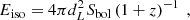 (2)
(2)
where Sbol is calculated from the observed fluence in the rest frame 1−10 000 keV energy band by assuming the Band function spectrum (Band et al. 1993)
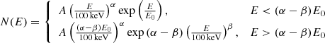 (3)
(3)
where Ep, z = (1 + z)Ep is the rest-frame peak energy, and Ep = (α + 2)E0 is the peak energy in the E2N(E) spectrum.
For the purpose of this work, we express the Amati relation as
 (4)
(4)
Here we adopt the GRB sample compiled in Demianski et al. (2017a,b), which includes 162 well-measured GRBs in the following redshift range: z ∈ [0.125, 9.3]. We divided the GRB sample into four sub-groups with different redshift bins, for example, 0.125 < z ≤ 1, 1 < z ≤ 2, 2 < z ≤ 3, and z > 3. The number of GRBs contained in the four subsamples is 42, 54, 35, and 30, respectively.
3. Calibration results for Amati relation using Hubble diagram of quasars
As the most luminous persistent sources in the Universe, quasars are bright enough to be detected up to redshifts z > 7 (Mortlock et al. 2011; Banados et al. 2018; Wang et al. 2018; Yang et al. 2020). According to the currently accepted model, quasars are extremely luminous active galactic nuclei (AGNs), where the observed intense energy release are related to the accretion of a gaseous disk onto a supermassive black hole (SMBH). Quasars have a wide spectral energy distribution, which normally contains a significant emission component in the optical-UV band LUV, the so-called big blue bump, with a softening at higher energies (Sanders et al. 1989; Elvis et al. 1994; Trammell et al. 2007; Shang et al. 2011). It has long been discussed that there is a nonlinear relationship between LUV and the quasar’s X-ray luminosity LX, parametrized as log(LX) = γlog(LUV)+β (Vignali et al. 2003; Strateva et al. 2005; Steffen et al. 2006; Just et al. 2007; Green et al. 2009; Young et al. 2010; Jin et al. 2012). From the theoretical point of view, this relation could be intrinsic since the UV emission is usually thought to originate from the optically thick disk surrounding the SMBH and the X-ray photons are thought to be generated through the inverse-Compton scattering of these disk UV photons by a plasma of hot relativistic electrons (the so-called corona) around the accretion disk. Such a relation is found to be independent of redshift (Lusso & Risaliti 2016), so that it could be used as a distance indicator to estimate cosmological parameters. The initial dispersion of the LUV − LX relation is relatively large (δ ∼ 0.35−0.4, Just et al. 2007; Young et al. 2010), but after a detailed study, Lusso & Risaliti (2016) suggest that most of the observed dispersion is not intrinsic, but it is rather due to observational effects. By gradually refining the selection technique and flux measurements, Risaliti & Lusso (2019) collected a complete sample of quasars, whose dispersion of the LUV − LX relation is smaller than 0.15 dex. The sample of main quasars is composed of 1598 data points in the range from 0.036 < z < 5.1. With this sample, they constructed a Hubble diagram of quasars in redshift range of 0.5 < z < 5.5, which is in excellent agreement with the analogous Hubble diagram for SNIa in the redshift range of 0.5 < z < 1.4. Moreover, this Hubble diagram of quasars has been studied in cosmological applications (Zheng et al. 2020, 2021). Considering that objects at the same redshift should have the same luminosity distance in any cosmology, here we first fit the model-independent cosmography formula that reflects the Hubble relation between the luminosity distance and redshif using the quasar sample, and then we obtained the distance moduli (also the luminosity distance) for GRBs at a given redshift with the best fit results.
It has long been proposed that the evolution of the universe could be described by pure kinematics, only relying on the assumption of the basic symmetry principles (the cosmological principle) that the universe can be described by the Friedmann-Robertson-Walker metric, but independent of any cosmology model (Weinberg 1972). In such a cosmography framework, the luminosity distance could be expressed as a power series in the redshift by means of a Taylor series expansion (Visser 2004)
![Mathematical equation: $$ \begin{aligned} d_{L}(z)&=cH_0^{-1}\left\{ z+\frac{1}{2}(1-q_0)z^2-\frac{1}{6}\left(1-q_0-3q_0^2+j_0\right.\right.\nonumber \\&\quad \left.\left.+\frac{kc^2}{H_0^2a^2(t_0)}\right)z^3+\frac{1}{24}\left[2-2q_0-15q_0^2-15q_0^3+5j_0\right.\right.\nonumber \\&\quad \left.\left.+10q_0j_0+s_0+\frac{2kc^2(1+3q_0)}{H_0^2a^2(t_0)}\right]z^4+\ldots \right\} \,, \end{aligned} $$](/articles/aa/full_html/2021/07/aa40895-21/aa40895-21-eq5.gif) (5)
(5)
where k = −1, 0, +1 corresponds to a hyperspherical, Euclidean, or spherical universe, respectively. The coefficients of the expansion are the so-called cosmographic parameters (e.g., Hubble parameters H, deceleration parameters q, jerk parameters j, and snap parameters s), which relate to the scale factor a(t) and its higher order derivatives:
 (6)
(6)
 (7)
(7)
 (8)
(8)
 (9)
(9)
All subscripts “0” indicate the present value of the parameters (t = t0). In order to avoid the convergence of the series at high redshift and to better control the approximation induced by truncations of the expansions, Cattoën & Visser (2007) proposed to use an improved parameter y = z/(1 + z) to recast the dL expression as
![Mathematical equation: $$ \begin{aligned} d_L({ y})&=\frac{c}{H_0}\Bigg \{{ y}-\frac{1}{2}(q_0-3){ y}^2+\frac{1}{6}\Bigg [12-5q_0+3q^2_0\nonumber \\&\quad -(j_0+\Omega _0)\Bigg ]{ y}^3+\frac{1}{24}\Bigg [60-7j_0-10\Omega _0-32q_0\nonumber \\&\quad +10q_0j_0+6q_0\Omega _0+21q^2_0-15q^3_0+s_0\Bigg ]{ y}^4+\mathcal{O} ({ y}^5)\Bigg \}\ , \end{aligned} $$](/articles/aa/full_html/2021/07/aa40895-21/aa40895-21-eq10.gif) (10)
(10)
where Ω0 is the total energy density. For the purpose of this work, here we fit the truncation of the dL expression (for the flat universe Ω0 = 1) to the second order term with the quasar sample. Our best cosmographic fitting result is

In our adopted sample, 156 GRBs are in the redshift range of 0.5 < z < 5.5. The luminosity distance for these GRBs were recalculated based on the best fitted cosmography formula, as was also the case for their isotropic equivalent energy in gamma-ray band.
With the newly calculated isotropic equivalent energy Eiso, we calibrated the Amati relation for each subsample and the whole sample. Here we make a logarithm linear fitting between Ep, z (in units of keV) and Eiso (in units of ergs) by adopting a likelihood function written as (Reichart et al. 2001)
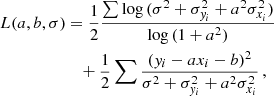 (11)
(11)
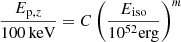
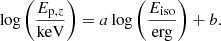
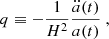
where xi = log(Eiso), yi = log(Ep, z), and σ marks the observational intrinsic dispersion. We adopted the Python package of emcee to perform the fitting and took the Uniform priors on a ∈ [0, 4], b ∈ [50, 56], and δ ∈ [0, 1]. The best fitting results for each subsample and the whole sample have been consolidated in Table 1 and plotted in Fig. 1. In the bottom panel of Fig. 1, we show the 1D marginalized distributions and 2D contours with the 1σ and 2σ confidence region. In Fig. 2, we plotted the best fitting values of coefficient a and b for each subsample with respect to the subsample’s mean redshift.
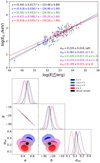 |
Fig. 1. Upper panel: fitting results for Amati relation with GRB samples in different redshift range (the black line is for the whole sample, the blue line is for 0.125 < z ≤ 1, the green line is for 1 < z ≤ 2, the purple line is for 2 < z ≤ 3, and the red line is for z ≥ 3), where the GRB distance moduli were calibrated by the quasar data. Lower panel: 1D marginalized distributions and 2D plots with 1σ and 2σ contours for luminosity correlation parameters. |
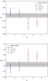 |
Fig. 2. Best fitting values of coefficient a (upper panel) and b (lower panel) for each subsample with respect to the subsample’s mean redshift. |
Best fitting values of coefficient a and b for each sub-sample.
Our results show that the best fitting values of a and b seem to have a certain redshift evolution. For coefficient a, the results of the first three subsamples (z < 3) are in good agreement with each other, however the result of the last high redshift subsample does not coincide with the previous ones in the range of 1σ. Even so, they still coincide in the range of 2σ. More interestingly, the best fitting values of coefficient b first increases and then decreases with the increase in the sample redshift. The variation range of the b value between different subsamples could reach 0.93%, and the result for the medium redshift range (1 < z < 3) does not coincide with the low or high redshift sample in range of 1σ. As shown in the lower panel of Fig. 1, parameters a and b are correlated, which is expected for a linear fit. There seems to be no evolution trend for the dispersion (denoted by the δ value) of the relation.
4. Discussion
Gamma-ray bursts are attractive cosmic probes due to their high redshift characteristics. Many empirical correlations between their isotropic energy/luminosity and some directly detectable spectral or temporal properties have been proposed, intending to shape GRBs into standard candles. However, unlike the Type Ia SNe, all these GRB luminosity relations lack definite physical explanations, mainly because our knowledge of the progenitor, central engine, and jet composition for GRBs are still limited. In this case, before applying GRBs to explore the universe, the properties of these relations need to be further examined. For example, whether there is redshift evolution for these relations is something worth studying. Using a complete quasar sample with a large redshift span to calibrate the isotropic equivalent energy of GRBs, here we find no significant evidence that the Amati relation has an evolution with redshift. Some previous methods, such as calibrating the luminosity relations of GRBs in the low redshift region and then extrapolating that to the high redshift region, may be problematic. It is worth noticing that the dispersion of the Hubble diagram for our adopted quasar sample is relatively large, which may bring some uncertainty as to the distance calibration, as well as to the fitting results for the Amati relation. Nevertheless, the method we have discussed here is universal. In the future, when the quasar sample quality becomes better or when there are other, better distance indicator samples with a large redshift span, we will study the redshift evolution of the GRB luminosity relation in more detail.
Acknowledgments
This work was supported by the National Natural Science Foundation of China under Grants Nos. 11633001, 11920101003, 12021003 and 11690024, the Strategic Priority Research Program of the Chinese Academy of Sciences, Grant No. XDB23000000 and the Interdiscipline Research Funds of Beijing Normal University.
References
- Amati, L. 2006, MNRAS, 372, 233 [Google Scholar]
- Amati, L., & Della, V. 2013, Int. J. Mod. Phys. D, 22(14), 1330028 [Google Scholar]
- Amati, L., Frontera, F., Tavani, M., et al. 2002, A&A, 390, 81 [NASA ADS] [CrossRef] [EDP Sciences] [Google Scholar]
- Amati, L., Guidorzi, C., Frontera, F., et al. 2008, MNRAS, 391, 577 [Google Scholar]
- Amati, L., D’Agostino, R., Luongo, O., et al. 2019, MNRAS, 486, L46 [Google Scholar]
- Banados, E., Venemans, B., Mazzucchelli, C., et al. 2018, Nature, 553, 473 [Google Scholar]
- Band, D., Matteson, J., Ford, L., et al. 1993, ApJ, 413, 281 [NASA ADS] [CrossRef] [Google Scholar]
- Cattoën, C., & Visser, M. 2007, Classical and Quantum Gravity, 24, 5985 [Google Scholar]
- Demianski, M., Piedipalumbo, E., Sawant, D., et al. 2017a, A&A, 598, A112 [NASA ADS] [CrossRef] [EDP Sciences] [Google Scholar]
- Demianski, M., Piedipalumbo, E., Sawant, D., et al. 2017b, A&A, 598, A113 [CrossRef] [EDP Sciences] [Google Scholar]
- Elvis, M., Wilkes, B. J., McDowell, J. C., et al. 1994, ApJS, 95, 1 [Google Scholar]
- Gao, H., Liang, N., & Zhu, Z.-H. 2012, Int. J. Mod. Phys. D, 21, 1250016-1 [Google Scholar]
- Gehrels, N., Chincarini, G., Giommi, P., et al. 2004, ApJ, 611, 1005 [NASA ADS] [CrossRef] [Google Scholar]
- Ghirlanda, G., Ghisellini, G., & Lazzati, D. 2004a, ApJ, 616, 331 [Google Scholar]
- Ghirlanda, G., Ghisellini, G., Lazzati, D., et al. 2004b, ApJ, 613, L13 [Google Scholar]
- Ghirlanda, G., Nava, L., Ghisellini, G., et al. 2009, A&A, 496, 585 [NASA ADS] [CrossRef] [EDP Sciences] [Google Scholar]
- Green, P. J., Aldcroft, T. L., Richards, G. T., et al. 2009, ApJ, 690, 644 [Google Scholar]
- Jin, C., Ward, M., & Done, C. 2012, MNRAS, 422, 3268 [NASA ADS] [CrossRef] [Google Scholar]
- Just, D. W., Brandt, W. N., Shemmer, O., et al. 2007, ApJ, 665, 1004 [Google Scholar]
- Khadka, N., & Ratra, B. 2020, MNRAS, 497, 263 [Google Scholar]
- Liang, E., & Zhang, B. 2005, ApJ, 633, 611 [Google Scholar]
- Liang, N., Xiao, W. K., Liu, Y., et al. 2008, ApJ, 685, 354 [Google Scholar]
- Lusso, E., & Risaliti, G. 2016, ApJ, 819, 154 [NASA ADS] [CrossRef] [Google Scholar]
- Montiel, A., Cabrera, J. I., & Hidalgo, J. C. 2021, MNRAS, 501, 3515 [Google Scholar]
- Mortlock, D., Warren, S., Venemans, B., et al. 2011, Nature, 474, 616 [Google Scholar]
- Muccino, M., Izzo, L., Luongo, O., et al. 2021, ApJ, 908, 181 [Google Scholar]
- Reichart, D. E., Lamb, D. Q., Fenimore, E. E., et al. 2001, ApJ, 552, 57 [Google Scholar]
- Risaliti, G., & Lusso, E. 2019, Nat. Astron., 3, 272 [Google Scholar]
- Salvaterra, R., Della Valle, M., Campana, S., et al. 2009, Nature, 461, 1258 [NASA ADS] [CrossRef] [PubMed] [Google Scholar]
- Sanders, D. B., Phinney, E. S., Neugebauer, G., et al. 1989, ApJ, 347, 29 [Google Scholar]
- Schaefer, B. E. 2007, ApJ, 660, 16 [Google Scholar]
- Shang, Z., Brotherton, M. S., Wills, B. J., et al. 2011, ApJS, 196, 2 [NASA ADS] [CrossRef] [Google Scholar]
- Steffen, A. T., Strateva, I., Brandt, W. N., et al. 2006, AJ, 131, 2826 [NASA ADS] [CrossRef] [Google Scholar]
- Strateva, I. V., Brandt, W. N., Schneider, D. P., et al. 2005, AJ, 130, 387 [Google Scholar]
- Tanvir, N. R., Fox, D. B., Levan, A. J., et al. 2009, Nature, 461, 1254 [Google Scholar]
- Trammell, G. B., Vanden Berk, D. E., Schneider, D. P., et al. 2007, AJ, 133, 1780 [Google Scholar]
- Vignali, C., Brandt, W. N., & Schneider, D. P. 2003, AJ, 125, 433 [NASA ADS] [CrossRef] [Google Scholar]
- Visser, M. 2004, Classical Quantum Gravity, 21, 2603 [Google Scholar]
- Vitagliano, V., Xia, J.-Q., Liberati, S., et al. 2010, J. Cosmol. Astropart. Phys., 2010, 005 [Google Scholar]
- Wang, F. Y., Dai, Z. G., & Zhu, Z.-H. 2007, ApJ, 667, 1 [Google Scholar]
- Wang, F. Y., Dai, Z. G., & Liang, E. W. 2015, New Astron. Rv., 67, 1 [Google Scholar]
- Wang, G.-J., Yu, H., Li, Z.-X., et al. 2017, ApJ, 836, 103 [Google Scholar]
- Wang, F.-G., Yang, J.-Y., Fan, X.-H., et al. 2018, ApJ, 869, L9 [Google Scholar]
- Wei, J.-J., Wu, X.-F., & Melia, F. 2013, ApJ, 772, 43 [Google Scholar]
- Weinberg, S. 1972, Gravitation and Cosmology: Principles and Applications of the General Theory of Relativity (Wiley-VCH), 688 [Google Scholar]
- Yang, J.-Y., Wang, F.-G., Fan, X.-H., et al. 2020, ApJ, 897, L14 [Google Scholar]
- Young, M., Elvis, M., & Risaliti, G. 2010, ApJ, 708, 1388 [Google Scholar]
- Zhang, B. 2018, The Physics of Gamma-Ray Bursts by Bing Zhang (Cambridge Univeristy Press), 2018 [Google Scholar]
- Zheng, X.-G., Liao, K., Marek, B., et al. 2020, ApJ, 892, 103 [Google Scholar]
- Zheng, X.-G., Cao, S., Biesiada, M., et al. 2021, Sci. China Phys. Mech. Astron., 64 [Google Scholar]
All Tables
All Figures
|
Fig. 1. Upper panel: fitting results for Amati relation with GRB samples in different redshift range (the black line is for the whole sample, the blue line is for 0.125 < z ≤ 1, the green line is for 1 < z ≤ 2, the purple line is for 2 < z ≤ 3, and the red line is for z ≥ 3), where the GRB distance moduli were calibrated by the quasar data. Lower panel: 1D marginalized distributions and 2D plots with 1σ and 2σ contours for luminosity correlation parameters. |
| In the text | |
|
Fig. 2. Best fitting values of coefficient a (upper panel) and b (lower panel) for each subsample with respect to the subsample’s mean redshift. |
| In the text | |
Current usage metrics show cumulative count of Article Views (full-text article views including HTML views, PDF and ePub downloads, according to the available data) and Abstracts Views on Vision4Press platform.
Data correspond to usage on the plateform after 2015. The current usage metrics is available 48-96 hours after online publication and is updated daily on week days.
Initial download of the metrics may take a while.