| Issue |
A&A
Volume 650, June 2021
|
|
|---|---|---|
| Article Number | A204 | |
| Number of page(s) | 14 | |
| Section | Astrophysical processes | |
| DOI | https://doi.org/10.1051/0004-6361/202140893 | |
| Published online | 30 June 2021 | |
General-relativistic instability in rapidly accreting supermassive stars: The impact of rotation
Département d’Astronomie, Université de Genève, Chemin des Maillettes 51, 1290 Versoix, Switzerland
e-mail: This email address is being protected from spambots. You need JavaScript enabled to view it.
Received:
26
March
2021
Accepted:
23
April
2021
Abstract
Context. Supermassive stars (SMSs) collapsing via the general-relativistic (GR) instability are invoked as the possible progenitors of supermassive black holes. Their mass and angular momentum at the onset of the instability are key in many respects, in particular regarding the possibility for observational signatures of direct collapse. Accretion dominates the evolution of SMSs and, similar to rotation, it has been shown to impact their final properties significantly. However, the combined effect of accretion and rotation on the stability of these objects is not known.
Aims. Here, we study the stability of rotating, rapidly accreting SMSs against GR perturbations and derive the properties of these stars at death.
Methods. On the basis of hylotropic structures, which are relevant for rapidly accreting SMSs, we define rotation profiles under the assumption of local angular momentum conservation in radiative regions, which allows for differential rotation. We account for rotation in the stability of the structure by adding a Newtonian rotation term in the relativistic equation of stellar pulsation, which is justified by the slow rotations imposed by the ΩΓ-limit.
Results. We find that rotation favours the stability of rapidly accreting SMSs as soon as the accreted angular momentum represents a fraction of f ≳ 0.1% of the Keplerian angular momentum. For f ∼ 0.3−0.5%, the maximum masses consistent with GR stability are increased by an order of magnitude compared to the non-rotating case. For f ∼ 1%, the GR instability cannot be reached if the stellar mass does not exceed 107 − 108 M⊙.
Conclusions. These results imply that, as in the non-rotating case, the final masses of the progenitors of direct collapse black holes range in distinct intervals depending on the scenario considered: 105 M⊙ ≲ M ≲ 106 M⊙ for primordial atomically cooled haloes and 106 M⊙ ≲ M ≲ 109 M⊙ for metal-rich galaxy mergers. The models suggest that the centrifugal barrier is inefficient to prevent the direct formation of a supermassive black hole at the collapse of a SMS. Moreover, the conditions of galaxy mergers appear to be more favourable than those of atomically cooled haloes for detectable gravitational wave emission and ultra-long gamma-ray bursts at black hole formation.
Key words: stars: massive / stars: rotation / stars: black holes
© ESO 2021
1. Introduction
The possibility for stars with masses ≳105 M⊙ to exist in a stable state of equilibrium has been considered for half a century, in connection with the physics of quasars (e.g., Hoyle & Fowler 1963b,a; Fowler 1966; Bisnovatyi-Kogan et al. 1967; Appenzeller & Kippenhahn 1971; Appenzeller & Fricke 1971, 1972a,b; Shapiro & Teukolsky 1979; Fuller et al. 1986; Baumgarte & Shapiro 1999b,a; Begelman 2010; Hosokawa et al. 2013; Umeda et al. 2016; Woods et al. 2017; Haemmerlé et al. 2018b,a, 2019; see Woods et al. 2019 and Haemmerlé et al. 2020 for recent reviews). One of the particularities of these supermassive stars (SMSs) is to end their life through the general-relativistic (GR) instability (Chandrasekhar 1964). The pressure support of SMSs is dominated by radiation (∼99%), so that these stars are always close to the Eddington limit. Since the Eddington limit corresponds to a state of marginal stability in Newtonian gravity, small GR corrections, of the order of a percent, are sufficient to make the star unstable with respect to radial pulsations. For Population III (Pop III) SMSs, the subsequent collapse is expected to lead to the direct formation of a supermassive black hole (Fricke 1973; Shapiro & Teukolsky 1979; Shibata & Shapiro 2002; Shapiro & Shibata 2002; Liu et al. 2007; Uchida et al. 2017; Sun et al. 2017, 2018).
Such direct collapse black holes are invoked to explain the existence of the most massive quasars observed around redshift 7 (e.g., Rees 1978, 1984; Volonteri & Begelman 2010; Volonteri 2010; Valiante et al. 2017; Zhu et al. 2020). The inferred black hole masses in these objects are in excess of 109 M⊙, so that accretion must have proceeded at average rates ≳1−10 M⊙ yr−1 because of the finite age of the Universe. The most studied channel of direct collapse is the case of primordial, atomically cooled haloes, in which mass inflows of 0.1–10 M⊙ yr−1 are expected below a parsec (e.g., Bromm & Loeb 2003; Dijkstra et al. 2008; Latif et al. 2013; Regan et al. 2016, 2017; Chon et al. 2018; Patrick et al. 2020). Larger inflows, up to ∼105 M⊙ yr−1, have been found in the simulations of the mergers of massive galaxies at redshifts 8–10 (Mayer et al. 2010, 2015; Mayer & Bonoli 2019). Such galaxies are thought to have experienced significant star formation, so that the progenitors of direct collapse black holes in this channel might be Population I (Pop I) SMSs. The hydrodynamical simulations of unstable SMSs show that for metallicities as high as solar, the collapse generally triggers a thermonuclear explosion that prevents black hole formation (Appenzeller & Fricke 1972a,b; Fuller et al. 1986; Montero et al. 2012). Only for masses ≳106 M⊙ does the deep potential well allow for gravity to bind the collapsing star. In both cases, direct collapse or supernova explosion, the high energies involved in the death of a SMS might allow for observational signatures of the existence of these objects. The simulations of collapsing Pop III SMSs suggest the possibility for gravitational wave emission and ultra-long gamma-ray bursts (Liu et al. 2007; Shibata et al. 2016a; Uchida et al. 2017; Sun et al. 2017, 2018; Li et al. 2018). But the detectability of such signatures sensitively depends on the mass and rotational properties of the SMS at collapse. In particular, both gravitational waves and gamma-ray bursts require spherical symmetry to be broken, so that rotation is crucial in that respect.
The properties of SMSs at the onset of GR instability have been studied in the case of polytropic structures (e.g., Fowler 1966; Bisnovatyi-Kogan et al. 1967; Baumgarte & Shapiro 1999a; Shibata et al. 2016b; Butler et al. 2018). Stars with masses ∼108 − 109 M⊙ are found to be stable, provided rapid enough rotation. Such structures correspond to fully convective, thermally relaxed stars, which are assumed to have formed at once (‘monolithic’ SMSs, Woods et al. 2020). They are found to feature universal rotational properties, in particular a universal value for the spin parameter, which is key regarding black hole formation and gravitational wave emission. But polytropic models become irrelevant when we account for the formation process of SMSs. The minimum accretion rates ∼1 M⊙ yr−1 that are required to explain the existence of the most massive and distant quasars are also necessary for the formation of a SMS, because the H-burning timescale near the Eddington limit is expected to be of the order of a million years, so that gathering 105 M⊙ before fuel exhaustion requires rates ≳0.1 M⊙ yr−1. Accretion at such rates critically impacts the structure of SMSs by preventing the thermal relaxation of their envelope (Begelman 2010; Hosokawa et al. 2012, 2013; Schleicher et al. 2013; Sakurai et al. 2015; Haemmerlé et al. 2018b, 2019). The high entropy in the outer regions stabilises most of the star against convection, which develops only in the inner ∼10% of the mass, triggered by H-burning. The stability of such structures against GR has been addressed in several works (Umeda et al. 2016; Woods et al. 2017; Haemmerlé 2020, 2021). SMSs accreting at rates from 0.1 to 10 M⊙ yr−1 are found to collapse at masses 1−4 × 10⁵ M⊙, while masses in excess of 106 M⊙ would require rates ≳1000 M⊙ yr−1. However, these results do not account for the effect of rotation.
Accretion onto a hydrostatic structure requires low enough angular momentum for the centrifugal force to be cancelled by an excess of gravity over the pressure forces. The rotation velocity of SMSs is constrained by the ΩΓ-limit (Maeder & Meynet 2000), which imposes velocities of less than ∼10% of the Keplerian values for masses ≳105 M⊙, due to the prominent role of radiation pressure in this mass range (Haemmerlé et al. 2018a; Haemmerlé & Meynet 2019). For such slow velocities, rotation hardly impacts the stellar structure and, in particular, rotational flattening is negligible. As we see later, the dynamical effects of rotation are of the same order as those of gas pressure and GR corrections, so that, similar to these effects, rotation plays a key role in the stability of the star, but can be neglected regarding its equilibrium properties.
In the present work, we use this advantage to define rotation profiles on the non-rotating structures of rapidly accreting SMSs on the basis of the hylotropic models of Begelman (2010). In the absence of convection, large differential rotation is expected to develop in the interior of SMSs (Haemmerlé et al. 2018a; Haemmerlé & Meynet 2019). Thus, while solid rotation must be imposed in the convective core, we assume that each radiative layer contracts with local angular momentum conservation. In Haemmerlé (2020), we applied the relativistic pulsation equation of Chandrasekhar (1964) to non-rotating hylotropes. Here, we add a term accounting for rotation to this equation, following the method of Fowler (1966), and apply it to the rotating hylotropes. The hydrostatic structures and rotation profiles are defined in Sects. 2.1 and 2.2, respectively. The rotation term for the GR instability is introduced in Sect. 2.3 (see also Appendix A). The numerical results are presented in Sect. 3 and their implications are discussed in Sect. 4. We summarise the main conclusions in Sect. 5.
2. Method
2.1. Hylotropic structures
Classical spherical stellar structures are determined by the equations of hydrostatic equilibrium and continuity of mass in the following form:
 (1)
(1)
 (2)
(2)
where r is the radial distance, Mr is the mass enclosed inside r, P is the pressure, ρ is the density of mass, and G is the gravitational constant. The structure is fully determined, provided an additional constraint of the form f(r, Mr, P, ρ) = 0, for example a constraint on the entropy profile: s(P, ρ) = s(Mr). In convective regions, where entropy is uniformly distributed, a constraint is given by s(Mr) = cst. But the entropy gradients that characterise radiative regions generally prevent from closing the equation system without the use of additional differential equations, energy transfer, and conservation.
For rapid enough accretion, the entropy profile of SMSs is well described by a hylotropic law (Begelman 2010; Haemmerlé et al. 2019; Haemmerlé 2020):
 (3)
(3)
where Mcore is the mass of the isentropic, convective core and sc is the specific entropy in the core. Equation (3) provides the required constraint s(P, ρ) = s(Mr) that closes (1) and (2), with a function s(P, ρ) given by the equation of state.
The entropy of SMSs is dominated by radiation,
 (4)
(4)
where T is the temperature and aSB is the Stefan-Boltzmann constant. The contribution from gas reduces to its contribution to pressure:
 (5)
(5)
where μ is the mean molecular weight, mH is the mass of a proton, and kB is the Boltzmann constant. This contribution is expressed by the following ratio (∼1%):
 (6)
(6)
Inserting Eq. (3) into Eq. (6), we obtain
 (7)
(7)
where  . Pressure can be expressed as a function of ρ and β instead of ρ and T, using the definition (6) of β to eliminate T in Eq. (5):
 (8)
(8)
Inserting Eq. (7) into Eq. (8), we obtain
 (9)
(9)
where
 (10)
(10)
The power-law (9) allows one to close the system (1) and (2), and thus to solve the stellar structure numerically for any length or mass scales, in a way similar to polytropes (Begelman 2010). To that aim, we define dimensionless functions ξ, θ, φ, and ψ as follows:
 (11)
(11)
The length scale is defined as a function of the central density and pressure
 (12)
(12)
where we used the fact that  (Eq. (9)). We notice that the mass scale is directly given by the constant K, that is to say by βc and μ (Eq. (10)). It can be written alternatively as
 (13)
(13)
In these dimensionless quantities, Eqs. (1) and (2) and constraint (9) read as follows:
 (14)
(14)
 (15)
(15)
 (16)
(16)
We see that, in contrast to polytropes, a free parameter remains in the dimensionless structure itself, φcore, the dimensionless mass of the convective core. Thus, exploring the full parameter space requires one to solve a series of structures, labelled by the various values of φcore in the interval 0.46–2.02. These two limits correspond to the limit of gravitational binding and to polytropic structures, respectively, where φsurf = φcore (Begelman 2010). As shown in Haemmerlé (2020), these Newtonian structures allow for a precise determination of the onset point of the GR instability in non-rotating, rapidly accreting SMSs, thanks to the weakness of GR corrections (≲1%).
2.2. Rotation profiles
Because SMSs are close to the Eddington limit, the rotation of their surface is constrained by the ΩΓ-limit (Maeder & Meynet 2000), which accounts for radiation pressure, instead of the Keplerian limit, based on the simple balance between gravity and the centrifugal force. The ΩΓ-limit is extremely restrictive for SMSs due to their high Eddington factor (0.9–0.99), and it implies surface velocities of ≲10% of the Keplerian velocity (Haemmerlé et al. 2018a):
 (17)
(17)
 (18)
(18)
For such velocities, the centrifugal acceleration represents less than a percent of the gravitational one:
 (19)
(19)
Interestingly, this dynamical contribution is of the same order as GR corrections and departures from the Eddington limit. Thus, similar to these effects, rotation shall play a significant role on the stability of SMSs, but it can be neglected in the definition of the hydrostatic structures.
Here, we use this advantage to define rotation profiles on the non-rotating hylotropes of Sect. 2.1. As a result of the short evolutionary timescales, angular momentum is expected to be locally conserved in the radiative envelope of SMSs (Haemmerlé et al. 2018a; Haemmerlé & Meynet 2019). Thus, we assume that the specific angular momentum of each radiative layer is given by that at accretion. Then, as the successive layers join the convective core, they advect this angular momentum, which is redistributed inside the core according to the constraint of solid rotation. We neglect the effect of the outer convective zone found in models of rapidly accreting SMSs (Hosokawa et al. 2013; Haemmerlé et al. 2018b). This envelope plays a negligible role in the GR instability as a result of its small mass and low density (Haemmerlé 2020). It plays a critical role in the rotation of the surface because its small mass covers large radii, over which angular momentum is instantaneously redistributed (Haemmerlé et al. 2018a; Haemmerlé & Meynet 2019). However, since it represents a percent of the total stellar mass, this redistribution impacts the angular momentum profile only locally once the layers contract in the radiative regions. Indeed, at each time, the specific angular momentum j− of the mass that leaves the envelope at its bottom r− is given by the angular velocity Ωenv of the envelope in solid rotation:
 (20)
(20)
where Menv, Jenv, and Ienv are the mass, the angular momentum, and the moment of inertia of the envelope, respectively, and ⟨jaccr⟩=Jenv/Menv is the average specific angular momentum advected at accretion by the layers of the envelope, which provides its angular momentum content. The large density contrasts in the envelope imply that most of its mass is located near r−, so that  and j− ≃ ⟨jaccr⟩. Since the layers of the envelope, over which the average ⟨ ⟩ is done, represent only a percent of the total mass, we can assume jaccr ≃ cst = ⟨jaccr⟩ for all these layers, so that the angular momentum j− advected by a layer in the radiative region is always close to what it advected at accretion: j− ≃ jaccr. In other words, regarding the inner rotation profiles, the convective envelope can be considered as a unique layer located in r−. Only when we consider the surface velocity does the depth of the envelope become important.
The accreted angular momentum is chosen as a fraction f of the Keplerian momentum at the equator
 (21)
(21)
where Raccr(M) is the accretion radius, that is to say the radius of the accretion shock when the star has a mass M. We use the mass-radius relation of rapidly accreting SMSs (Hosokawa et al. 2012, 2013; Haemmerlé et al. 2018b, 2019):
 (22)
(22)
This power-law, which reflects the evolution along the Eddington and Hayashi limits, reproduces the models well for masses ≲105 M⊙. Possible departures from this relation at larger masses are discussed in Sect. 4.2. The dependence R ∝ M1/2 implies a constant surface gravity as follows:
 (23)
(23)
The initial angular momentum of each layer Mr, which is conserved until it joins the core, is given by the angular momentum advected at the accretion of the layer (Eq. (21)), when the mass of the star was M = Mr:
 (24)
(24)
With the mass-radius relation (22), it is given uniquely by the mass-coordinate Mr of the layer and the fraction f:
 (25)
(25)
The angular velocity in the radiative envelope is then given by
 (26)
(26)
where we used the Keplerian velocity (18) and the local gravitational acceleration g = GMr/r2. We see that the ratio of Ω to its Keplerian value is given uniquely by f and the local gravity. The total angular momentum of the core is the integral of the angular momentum advected by the layers Mr < Mcore:
 (27)
(27)
From the assumption of solid rotation, the angular velocity of the core is
 (28)
(28)
where Icore, the moment of inertia of the core, is given by the non-rotating structure.
In order to apply these rotation profiles to the dimensionless hylotropic structures of Sect. 2.1, we rewrote them with the use of the dimensionless functions (11). The gravitational acceleration reads as follows:
 (29)
(29)
It is fully determined by the dimensionless structure (ξ, φ) and the central pressure. At first order, the central pressure is given by radiation, and thus it depends on the central temperature only. The rotation profile in the radiative envelope is given by (Eq. (26)) the following:
 (30)
(30)
From Eq. (27), the angular momentum of the core is
 (31)
(31)
By definition, the moment of inertia is given by
 (32)
(32)
Equation (28) gives
 (33)
(33)
The ratio to the Keplerian velocity (Eq. (18))
 (34)
(34)
is
 (35)
(35)
Thus, if we define
 (36)
(36)
 (37)
(37)
we can write the full rotation profile, that is to say the core plus envelope, in the following way:
 (38)
(38)
The gravity-ratio  is given uniquely by the central pressure, that is by the central temperature, while the dimensionless profile
  is given uniquely by the dimensionless hylotropic structure. Thus, for a given hylotrope, the profile of Ω/ΩK is given uniquely by the fraction f and the central temperature. We notice that for the central temperatures of SMSs (107 − 108 K), the gravity ratio
  takes values of ∼106, which reflects the strong contraction of the central layers of SMSs from their large accretion radii (22). Equation (38) suggests that typical values of f ∼ 0.1−1% are required for the typical velocities of ∼0.1ΩK imposed by the ΩΓ-limit. The Ω-profile additionally requires the scaling factor for ΩK, given by central density (Eq. (34))
 (39)
(39)
where
 (40)
(40)
From these rotation profiles, we can derive the profiles of the spin parameter:
 (41)
(41)
 (42)
(42)
We can see that the scaling factor of the spin parameter is given by the mass scale and the fraction f. In the radiative envelope (Mr > Mcore), the spin parameter can be directly obtained by integration of Eq. (25):
 (43)
(43)
Since convection only redistributes the angular momentum in the core, the amount Jr included in the mass Mr remains unchanged, and it is set directly by the accretion law (21), independently of the hylotropic structure. The choice of the structure impacts the spin parameter only in the core. For Mr < Mcore, Eq. (42) gives
 (44)
(44)
where  is the moment of inertia of the mass Mr. We see that the spin parameter is changed by a factor that depends on the two dimensionless ratios Mr/Mcore and Ir/Icore, uniquely given by the dimensionless structure. Thus, the full profile of the spin parameter, in the core and the envelope, is given by the dimensionless structure, the fraction f, and the mass scale.
Finally, the rotational kinetic energy is given by (Eq. (A.25))
 (45)
(45)
Its ratio to the absolute value of the gravitational energy
 (46)
(46)
corresponds to the average of  weighted on the gravitational energy per mass unit. With the rotation profile (38), we obtain
 (47)
(47)
where we used Eq. (15) to substitute dξ to dφ in the integrals. Since EΩ/|W| is an average of  , these two quantities share the same scaling factor. As a consequence, the profile of Ω/ΩK (Eq. (38)) is fully determined by EΩ/|W| and the dimensionless structure:
 (48)
(48)
Equation (48) suggests EΩ/|W|∼0.01 for the velocities of ∼0.1ΩK of the ΩΓ-limit.
2.3. Impact of rotation on the GR instability
The relativistic equation for the frequency ω of adiabatic pulsations was derived by Chandrasekhar (1964) from Einstein’s equations in full generality, with the only assumption of spherical symmetry. In Haemmerlé (2020, 2021), we have shown that this equation allows one to determine, with a high precision, the stability of any spherical (i.e. non-rotating) hydrostatic structure with respect to GR, if used in the following form:
 (49)
(49)
with
 (50)
(50)
 (51)
(51)
 (52)
(52)
 (53)
(53)
 (54)
(54)
where ′ indicates the derivatives with respect to r (r = R at the surface), Γ1 is the first adiabatic exponent, and a and b are the coefficients of the metric ds2 = −e2a(cdt)2 + e2bdr2 + r2dΩ2, given by the following:
 (55)
(55)
 (56)
(56)
Thanks to the weakness of GR corrections in SMSs, we can restrict our analysis to the first order post-Newtonian component of Eq. (49). Moreover, due to the proximity with the Eddington limit, Eq. (49) can be linearised in β, using the following expression for Γ1 (Haemmerlé 2020):
 (57)
(57)
In Haemmerlé (2020), we show that the first order post-Newtonian and sub-Eddington components of integrals (51)–(54) can be written in the following form with the help of the dimensionless functions defined in Eq. (11):
 (58)
(58)
 (59)
(59)
 (60)
(60)
 (61)
(61)
The dimensionless parameter σ, defined by (Tooper 1964)
 (62)
(62)
represents the departures from the Newtonian limit, while βc represents the departures from the Eddington limit. Integrals (58)–(61) have been obtained by linearisation with respect to these two parameters, that is to say neglecting terms in 𝒪(σ2),  , or 𝒪(σβc). The compactness is related to σ by
 (63)
(63)
Since all integrals (58)–(61) have a global σ or βc factor in front, their content can be evaluated with Newtonian equations. In particular, Eqs. (14)–(15) and an integration by parts allow one to write
 (64)
(64)
 (65)
(65)
so that
 (66)
(66)
Thus, in the post-Newtonian and sub-Eddington limit, the sum (49) of the integrals reduces to
 (67)
(67)
This sum can be re-expressed in terms of physical quantities, using Eqs. (11)–(12) and (62):
 (68)
(68)
 (69)
(69)
Using the volume dV = 4πr2dr and dMr from Eq. (2), the equation becomes
 (70)
(70)
where  reduces to the moment of inertia in the Newtonian limit.
Equation (70) contains all the terms that are required to capture the GR instability on any hydrostatic structure in the post-Newtonian and sub-Eddington limit, in the case of pure spherical symmetry, that is without rotation. The condition for the instability is an imaginary frequency of ω2 < 0. Since I is always positive, it happens when the negative term on the right-hand side, which contains the GR corrections in c−2, exceeds, in absolute value, the positive term, which contains β, the departures from the Eddington limit. This positive term is purely Newtonian since crossed GR and β corrections would give only second-order terms. Since β is the ratio of gas to the total pressure, this integral actually corresponds to the integrated gas pressure, which is two-thirds of the total internal energy contained in the gas. On the other hand, the negative integral, which scales with the GR corrections, also scales with the total gravitational energy of the star since the integrand scales with the gravitational energy per mass unit −GMr/r.
Since both β and the GR corrections have typical values of 0.01 in SMSs, the positive and negative integrals in Eq. (70) represent about a percent of the total internal and gravitational energies, respectively. As we have seen in Sect. 2.2, the dynamical contribution by rotation is of the same order. Thus, similar to the effect of gas pressure, the effect of rotation on the stability of the star can be reduced to its Newtonian component since relativistic rotation terms would be of second order. This method has been used by Fowler (1966), Bisnovatyi-Kogan et al. (1967), and Baumgarte & Shapiro (1999a) for polytropic models. For slow rotation near the Eddington limit, a Newtonian pulsation analysis leads to (see Appendix A, Eq. (A.21)) the following:
 (71)
(71)
The Ω2-term in Eq. (71) is the rotational energy (45) multiplied by a factor of 4/3. Since this term is positive, we see that rotation acts as a stabilising agent, similar to gas pressure, against the destabilising GR effects. It is expressed by adding this term in the post-Newtonian Eq. (70):
 (72)
(72)
In the sum of the Ii that appears in Eq. (49), this term translates into a fifth integral:
 (73)
(73)
With the rotation profiles defined in Sect. 2.2 (Eq. (38)), it gives
 (74)
(74)
Adding this term to Eq. (67), we obtain
 (75)
(75)
We see that the rotation term scales with the independent fraction f2, and with the square root of the gravity ratio  . From its definition (36),
  scales with
  , that is with the central temperature:
 (76)
(76)
The product of the other two scaling factors, βc and σ, is also given by the central temperature and the chemical composition:
 (77)
(77)
by definitions (6)–(62). Thus, the limit of stability, at which the right-hand side of Eq. (75) vanishes, is given by a second-order polynomial equation in βc:
 (78)
(78)
where the integral ratios
 (79)
(79)
 (80)
(80)
are uniquely given by the dimensionless structure  . The ratio
  corresponds to the critical ratio βc/σ in the non-rotating case (Haemmerlé 2020), while
  gives the correction from rotation. Equation (78) has a unique positive root of
 (81)
(81)
From Eq. (10), the corresponding mass scale (13) is directly given by  and the chemical composition μ:
 (82)
(82)
Thus, the critical masses for the star and its core
 (83)
(83)
 (84)
(84)
are uniquely determined by the dimensionless structure  and the choice of (f, Tc, μ).
In the case where f = 0, when the stability limit is set by gas only, Eq. (81) leads to  . In the opposite limit, when the stability is dominated by the effect of rotation,
 (85)
(85)
a linear development of Eq. (81) gives
 (86)
(86)
Expression (86) of βc,crit is independent of Tc, which implies that for large f, the critical mass scale (82) is independent of Tc and μ:
 (87)
(87)
In other words, in the limit of large f, the critical mass of a given hylotrope is set uniquely by f. This fraction appears to the power 4 in Eq. (87), which shows the strong dependence of the critical masses on the accreted angular momentum. Moreover, it implies that for large f, the profile of the spin parameter (Eq. (42)) at the limit of stability is independent of f, and is given uniquely by the following dimensionless structure:
 (88)
(88)
In particular, at the surface, there is the following:
 (89)
(89)
We emphasise, however, that this universality is broken when gas plays a significant role in the determination of the stability limit.
Finally, we notice that the critical condition (81) can be expressed as a function of EΩ/|W| (Eq. (47)) instead of f:
 (90)
(90)
with
 (91)
(91)
The integral at the numerator has been transformed by an integration by parts, using Eq. (14).
3. Results
3.1. Rotation profiles
The dimensionless rotation profiles of Eq. (40) are shown in Fig. 1 for a choice of hylotropes with the indicated values of φcore. The convective core, where solid rotation is imposed, clearly appears in each profile. In particular, the case φcore = 2.02, which corresonds to the polytropic limit, is fully rotating as a solid body. In contrast, strong differential rotation appears in the envelope of the other models; and for φcore ≲ 1, the angular velocity in the core exceeds, by several orders of magnitude, that of the surface, consistently with the models accounting for full stellar evolution (Haemmerlé et al. 2018a; Haemmerlé & Meynet 2019). We also see that the instantaneous angular momentum transport in the core introduces a discontinuity in the  -profiles at the interface with the envelope. Physically, such infinite gradients shall be smoothed out by shears, but here we can assume that such shears only lead to a local redistribution of the angular momentum, without a significant impact on the rotation profiles.
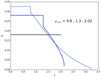 |
Fig. 1. Dimensionless rotation profiles of Eq. (40) for a set of hylotropes with the indicated values of φcore. |
From these dimensionless rotation profiles, the profiles of Ω/ΩK (Eq. (38)) are given by the ratio EΩ/|W| (Eq. (48)). They are shown in Fig. 2 for EΩ/|W| = 0.01. We see that the maximum values of Ω/ΩK are always reached at the surface of the convective core. The rotation velocity typically remains at 0.1–0.2 ΩK, except in the very outer layers of the polytropic model (φcore = 2.02). In this case, the ΩΓ-limit shall be exceeded at the surface, which shows that accretion onto fully convective SMSs requires EΩ/|W|≪0.01. On the other hand, the models with φcore ≲ 2 keep a surface velocity of ∼0.1ΩK, which is consistent with the ΩΓ-limit. We see that for a given constraint on the surface velocity, hylotropic structures allow for larger EΩ/|W|, thanks to differential rotation in the envelope. However, as already noticed in Sect. 2.2, the surface rotation of rapidly accreting SMSs depends on the depth of their convective envelope, which is not included in the hylotropic structures. The constraint on f that arises from this effect is discussed in Sect. 4.1.
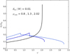 |
Fig. 2. Profiles of Ω/ΩK (Eq. (48)) for EΩ/|W| = 0.01, for a set of hylotropes with the indicated values of φcore. |
3.2. Critical masses
The critical masses obtained with Eqs. (83)–(84) for the full series of hylotropes are shown in Fig. 3 for Tc = 1.8 × 10⁸ K, μ = 0.6, and a series of values of the fraction f. These values of Tc and μ are relevant for Pop III SMSs (Hosokawa et al. 2013; Umeda et al. 2016; Woods et al. 2017; Haemmerlé et al. 2018b, 2019). In Fig. 4, the critical masses are shown for the lower Tc = 8.5 × 10⁷ K relevant for Pop I SMSs (Haemmerlé et al. 2019). For these central temperatures, the central densities are typically a few g cm−3 for M ∼ 105 − 106 M⊙, down to ∼0.01−0.1 g cm−3 for M ∼ 108 − 109 M⊙.
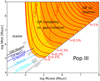 |
Fig. 3. Limits of stability for Pop III SMSs accreting angular momentum at a fraction f of the Keplerian momentum. The solid red lines show the hylotropic limits for the indicated f (Eq. (81)), with Tc = 1.8 × 10⁸ K and μ = 0.6, relevant for Pop III SMSs. The dotted red lines indicate the limit of stability for constant ratios 0.001–0.01–0.1 of rotational to gravitational energy (Eq. (90)). The coloured areas reflect the relative contribution by gas and rotation in the determination of the stability limit (81): From yellow to red, the rotation term |


As in the non-rotating case (Haemmerlé 2020), for every given f, the maximum total mass consistent with GR stability is a decreasing function of the core mass fraction. We see that the effect of rotation on the stability of the star becomes significant as soon as f ≳ 0.1%. For f = 0.2−0.3%, the mass limit is shifted by a significant factor, and for f = 0.3−0.5% by an order of magnitude. In this last case, the GR instability requires masses ≳106 M⊙. For f = 1%, the GR instability cannot be reached if the mass does not exceed several 107 M⊙, and the star can be stable with masses ∼109 M⊙ if the core does not exceed 106 M⊙. In the range of f = 1.5−2%, the star remains stable up to masses of 108 − 109 M⊙ for any core mass. We notice the small knee of the mass limits near the polytropic structures (Mcore ≳ 75%M). The stabilising effect of rotation is slightly decreased by the solid rotation of the core, which removes angular momentum from the densest central regions that are dominant for the instability.
The relative contribution by gas and rotation in the determination of the stability limit is made visible by coloured areas. These contributions are estimated by the two terms that appear in the critical condition (81):  , which represents gas, and
  , which represents rotation. The four regions, from yellow to red, correspond to the cases where the rotation term represents < 0.1, 0.1−1, 1−10, and > 10 times the gas term. We see that for 0.1%≲f ≲ 1%, both gas and rotation play a role in the determination of the stability limit. But for f ≳ 1%, rotation becomes the only significant stabilising effect (condition 85). In this case, as noticed in Sect. 2.3, the critical masses of the various hylotropes are uniquely given by f, independently of the thermal properties (Eq. (87)). As a consequence, the effect of a change in the central temperature, between Figs. 3 and 4, impacts the mass limits only for f ≲ 1%, while the limits for f ≳ 1% remain unchanged.
The mass limits obtained for constant EΩ/|W| (Eq. (90)) are shown in Figs. 3 and 4 as red dotted lines for EΩ/|W| = 0.001−0.01−0.1. Since the ratio EΩ/|W| scales with f2 (Eq. (47)), the range of one order of magnitude in f ∼ 0.1−1% corresponds to a range of two orders of magnitude in EΩ/|W|∼0.001−0.1. For Mcore > 10%M, the ratio EΩ/|W| = 0.01 corresponds to f ∼ 0.3−0.4%. The fastest rotators shown in these figures (f ∼ 1%) have EΩ/|W|∼0.1, which corresponds to typical velocities ∼0.3ΩK (Eq. (48)). We see that for a given value of EΩ/|W|, hylotropic structures with small Mcore/M remain stable up to larger masses than polytropes (Mcore = M). More precisely, for a given relative contribution EΩ/|W|, rotation has a stronger stabilising effect on hylotropes with Mcore < M than on polytropes. It reflects the fact that rotational energy is more centralised when the core is smaller (Fig. 2), and thus it has a stronger impact on the dense regions that are relevent for the GR instability.
3.3. Spin parameter
The profile of the spin parameter is given by Eq. (42). For each hylotrope, it is fully determined by the fraction f and the mass scale. As is noticeable in Sect. 2.2, f and the mass scale appear in Eq. (42) as global factors only, so that a change in these quantities affects only the scale of the spin parameter, while the shape of the profile is unique for each hylotrope. Here, we are interested in the profiles of the spin parameter at the limit of stability, where the mass scale is fixed by f, Tc, and μ Eqs. (81) and (82). Since the critical mass scale is not the same for the various hylotropes, the profiles of the spin parameter at the critical limit are rescaled by a different factor when f, Tc, and μ are changed.
The critical profiles obtained for f = 0.2%, Tc = 1.5 × 10⁸ K, and μ = 0.6 are shown in Fig. 5 for three hylotropes in the series. The case f = 1%, Tc = 9 × 10⁷ K, and μ = 0.6 is shown in Fig. 6. The profiles are compared with that of the angular momentum accretion law (25), expressed in Eq. (43). By construction, the profiles match each other in the radiative envelopes, and they are impacted by the stellar structure only in the convective core. By definition, the spin parameter diverges at the centre, but we see that for all the profiles, it decreases below unity at a small fraction of the total mass. The profile set by the accretion law, and kept in the envelope, is monotonously decreasing. Thus, if the spin parameter goes below unity in the deep regions of the envelope, it necessarily remains so in the whole envelope. Only in the convective core, where solid rotation redistributes the angular momentum, can the spin parameter increase outwards, which is in agreement with the polytropic models (Baumgarte & Shapiro 1999a). However, it occurs only for hylotropes with φcore ≳ 1, that is for a core mass fraction ≳40%.
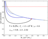 |
Fig. 5. Internal profile of the dimensionless spin parameter at the limit of stability for f = 0.2%, Tc = 1.5 × 10⁸ K, and μ = 0.6, as a function of the mass-coordinate and for a choice of hylotropes with indicated φcore. The surface of each hylotrope is indicated by a white square. The black dashed curve shows the angular momentum accretion law (43). The red dashed curve and the red square indicate the limits for black hole formation, according to the criterions discussed in Sect. 4.3. |
We notice that in these two cases, f = 0.2% and 1%, the stability limit is set predominantly by gas and by rotation, respectively (Figs. 3 and 4). Condition (85) is already satisfied for f = 1%, so that the critical profiles shown in Fig. 6 actually correspond to the ‘universal’ profiles of Eq. (88), independent of f and given uniquely by the dimensionless structure. As a consequence, these profiles represent an upper limit for each hylotrope, and the increase of the critical masses for f > 1% only translates into a rescaling along the x-axis. In particular, in the case of the polytrope (φcore = 2.02), we refind the profile of Baumgarte & Shapiro (1999a), with the ‘universal’ value 0.87 at the surface, given by Eq. (89).
4. Discussion
4.1. Final mass as a function of the accretion history
Figures 3 and 4 show that the maximum masses consistent with GR stability sensitively depend on the fraction f of accreted angular momentum, already in the range 0.1–1%. The actual value of f at which a SMS can accrete is set by the ΩΓ-limit, which imposes an upper limit for its surface velocity. For stars with masses ≳105 M⊙, the surface velocity cannot exceed ∼10% of the Keplerian velocity (Haemmerlé et al. 2018a; Haemmerlé & Meynet 2019). An extrapolation of the models suggests that the limit goes down to ∼3% for ≳107 M⊙, and to ∼1% for ≳109 M⊙. As noticed in Sect. 2.2, for a given fraction f of accreted angular momentum, the surface velocities of rapidly accreting SMSs depend on the depth of their convective envelopes, which are not included in the hylotropic models. Models accounting for full stellar evolution show that this envelope covers more than two-thirds of the total stellar radius for rates ≲1 M⊙ yr−1, which implies f ≲ 0.2−0.3% (Haemmerlé & Meynet 2019). On the other hand, the depth of the envelope is significantly reduced for rates ≳100 M⊙ yr−1, and it covers a small fraction of the total radius. As long as it remains the case, the SMS can accrete angular momentum at f ∼ 1% up to ∼109 M⊙ without facing the ΩΓ-limit.
Rapidly accreting SMSs are invoked in two different versions of direct collapse: atomically cooled haloes and galaxy mergers. The accretion rates in atomically cooled haloes are expected to be 0.1−10 M⊙ yr−1 and most probably ≲1 M⊙ yr−1 (Latif et al. 2013; Chon et al. 2018; Patrick et al. 2020), which imposes f ≲ 0.2−0.3%. On the other hand, galaxy mergers allow for rates ≳100 M⊙ yr−1 (Mayer et al. 2010, 2015; Mayer & Bonoli 2019), for which f ≃ 1% remains consistent with the ΩΓ-limit up to large masses. Another difference between these two scenarios is the chemical composition, which is primordial in atomically cooled haloes, while solar metallicities are expected in the case of galaxy mergers. Black hole formation at the collapse of a Pop I SMS requires a mass ≳106 M⊙ (Montero et al. 2012). In the non-rotating case, such final masses could be reached only for rates ≳1000 M⊙ yr−1 (Haemmerlé 2020, 2021).
The evolutionary tracks of the GENEC models accounting for full stellar evolution (Haemmerlé et al. 2018b, 2019), computed under accretion at 0.1–1000 M⊙ yr−1 up to masses of 105 − 106 M⊙, are plotted in Figs. 3 and 4. These models were built on the assumption of hydrostatic equilibrium, and thus they are insensitive to dynamical instabilities. Their stability with respect to GR perturbations has been addressed in Haemmerlé (2021) for the non-rotating case by the direct use of Eq. (49). As is shown in Haemmerlé (2020), the hylotropic limit reproduces these final masses with a high precision for accretion rates ≥10 M⊙ yr−1 and remains a good approximation for lower rates. We see that none of these tracks reach the stability limits for f ≳ 0.2%. An extrapolation of the tracks suggests that for conditions of atomically cooled haloes (Pop III, Ṁ ∼ 0.1 − 1 M⊙ yr−1, f ∼ 0.2−0.3%), rotation allows one to increase the final mass by a factor of ∼2 only. It implies that the mass of SMSs forming in this scenario always remain < 106 M⊙, and more probably ≲5 × 10⁵ M⊙. On the other hand, for the conditions of metal-rich galaxy mergers (Pop I, Ṁ ≳ 100 M⊙ yr−1, f ∼ 1%), rotation could allow SMSs to increase their final mass by several orders of magnitude, leading to an upper mass limit of 108 − 109 M⊙. Overall, as in the non-rotating case, the final masses of SMSs range in distinct intervals in the two versions of direct collapse: 105 − 106 M⊙ for atomically cooled haloes and 106 − 109 M⊙ in galaxy mergers. We notice also that the minimum rate required for final masses ≳106 M⊙ is slightly reduced by rotation, since for 100 M⊙ yr−1 already, we can expect f ∼ 1%.
Interestingly, an extrapolation of the tracks at Ṁ ≳ 100 M⊙ yr−1 in Figs. 3 and 4 suggests that stars accreting at these rates are mostly convective when they reach the GR instability for f ≃ 1%. The same is true for Ṁ ≲ 0.1 M⊙ yr−1 and f = 0.2%. If the star becomes fully convective before the instability, the instantaneous angular momentum transport affects the surface velocity, and the values of f consistent with the ΩΓ-limit decrease below < 0.1. Thus, either the accreted angular momentum decreases, so that the star rapidly becomes GR unstable, or the surface reaches break-up. In this case, accretion must stop and the star evolves along the mass-shedding limit, in a similar pathway as monolithic models (Fowler 1966; Bisnovatyi-Kogan et al. 1967; Baumgarte & Shapiro 1999a). In this case, only second-order post-Newtonian corrections have been found to trigger the collapse (Bisnovatyi-Kogan et al. 1967). We emphasise, however, that in the accretion scenario considered here, these second-order corrections always remain negligible, and we checked numerically that they do not play a role in the determination of the limits in Figs. 3 and 4. It is also important to notice that the age of a star accreting at 100–1000 M⊙ yr−1 when it reaches 108 − 109 M⊙ is ∼106 years, at which H-burning might be achieved (Umeda et al. 2016; Woods et al. 2021). In this case, pair-instability might be reached before the GR instability (Woods et al. 2020).
4.2. Angular momentum accretion law and rotation profiles
The definition of the rotation profiles in Sect. 2.2 relies on the angular momentum accretion law (21) and the mass-radius relation (22). This relation is verified by stellar evolution models for masses ≲105 M⊙ (Hosokawa et al. 2013; Haemmerlé et al. 2018b), but for larger masses the models depart towards smaller radii. In the absence of stellar evolution models accounting for accretion up to masses ≥106 M⊙, the mass-radius relation is not known for the most massive objects considered in the present work. According to Eq. (24), smaller radii would imply a slower rotation. However, the radius appears in this equation through its square root, so that a decrease by an order of magnitude in radius would be equivalent to a decrease by a factor of a few only in f. Moreover, the mass-radius relation of the zero-age main-sequence (ZAMS) imposes a lower limit to the radius. Similar to the Hayashi line, the ZAMS of SMSs follows a nearly constant effective temperature (Woods et al. 2020), leading to the same power-law R ∝ M1/2 as Eq. (22), rescaled down by 2–3 orders of magnitude in radius. Such a shift would be equivalent to a decrease in f by one order of magnitude. Since departures from relation (22) might appear only for M ≳ 106 M⊙, we can estimate that this effect would translate, in the (Mcore, M) diagram of Figs. 3 and 4, into a shift of the mass limits for f ≳ 0.5%, and down to f = 0.4%. We notice however that more recent models of very-massive stars show a shift in the ZAMS towards lower effective temperatures and larger radii (Gräfener 2021). This effect might inhibit a possible contraction of SMSs in the mass range ≳106 M⊙, allowing for accretion of relatively high angular momentum.
In addition to the mass-radius relation, the definition of the rotation profiles in Sect. 2.2 relies on the assumption of local angular momentum conservation in the envelope, which leads to strong differential rotation. Stellar models (Haemmerlé et al. 2018a) have shown shear diffusion and meridional circulation to be inefficient in rapidly accreting SMSs because of the short timescales and slow rotations. On the other hand, magnetic fields (e.g., a Taylor-Spruit dynamo), which are neglected in the present work, could inhibit significantly differential rotation. In the extreme case of solid rotation, the constraint from the ΩΓ-limit at the surface translates into f < 0.1%, and the effect of rotation on the stability becomes negligible. In other words, for given surface velocities, solid rotation would impose a low angular momentum in the deep regions of the star that are decisive for the GR instability, and this could bring back the stability limit to the non-rotating case.
We also notice that the ratio Ω/ΩK remains < 0.7 for all the rotation profiles considered (f ≲ 2%), except in the very outer layers of the nearly-polytropic models (Mcore/M > 0.95), which play a negligible role in the GR instability. No significant flattening is expected for such slow rotations (Ekström et al. 2008), which justifies the use of the spherical hylotropic structures. Moreover, in the deep regions that are relevent for the GR instability, the ratio  typically remains between 0.1–0.2. Thus, we can estimate that post-Newtonian rotation terms in the pulsation Eq. (72), which are neglected in the present method, should remain small compared to the other terms.
4.3. Spin parameter and black hole formation
The spin parameter (41) is key for the direct formation of a supermassive black hole during the collapse of a SMS. Without angular momentum transport, the profile ar(Mr) at the onset of the instability is conserved during the collapse. For monolithic SMSs, evolving along the mass-shedding limit and fully stabilised by rotation (condition (85)), analytical models in the post-Newtonian limit feature a universal profile of the spin parameter, with a unique value of 0.87 at the surface in particular (Baumgarte & Shapiro 1999a). Except in the central ∼10% of the mass, the spin remains always ar < 1, the maximum value allowed for the formation of a Kerr black hole, which suggests that the whole stellar mass can be accreted by the black hole in a dynamical time. We notice that since monolithic models are rotating at the Keplerian limit, the conditions for a Newtonian treatment of rotation are not satisfied, and the full GR numerical simulations of Baumgarte & Shapiro (1999a) lead to larger values for the spin parameter (0.97). Only the slow rotations imposed by accretion along the ΩΓ-limit guarantee the validity of the Newtonian treatment of rotation against GR instability.
The hydrodynamical simulations of the collapse of monolithic SMSs have shown that the outer ∼10% of the stellar mass remains in orbit outside the horizon (Shibata & Shapiro 2002; Shapiro & Shibata 2002; Liu et al. 2007; Uchida et al. 2017; Sun et al. 2017, 2018). The resulting non-axisymmetric structure is found to trigger gravitational wave emission and ultra-long gamma-ray bursts, which are currently the main observational signatures of the existence of SMSs proposed in the literature for future detection. Shapiro & Shibata (2002) showed that the mass of the orbiting structure in the simulations can be derived analytically by comparing the specific angular momentum of each layer Mr with that of the innermost stable circular orbit (ISCO) of a black hole with mass Mr and spin ar: if the angular momentum exceeds the ISCO value in a layer, the layer remains in orbit outside the horizon.
The critical profiles of the spin parameter shown in Figs. 5 and 6 correspond to typical conditions of atomically cooled haloes and galaxy-mergers, respectively. For conditions of galaxy mergers, we refind the profile of Baumgarte & Shapiro (1999a) for the polytrope (φcore = 2.02), which reflects the fact that condition (85) is already satisfied for f = 1%. In contrast, for the case of atomically cooled haloes (f = 0.2%, Fig. 5), gas plays the dominant role in setting the stability limit (Fig. 3), and the spin parameter departs from the ‘universal’ profiles, as already noticed by Shibata et al. (2016b) and Butler et al. (2018) for monolithic models. By comparing the angular momentum profiles with the ISCO values of the various layers (Eq. (17) of Shapiro & Shibata 2002), we can estimate in which cases an outer envelope rotates fast enough to remain in circular orbit after black hole formation. The limit of this envelope is shown by a red square in the profiles, and we see that it only occurs for nearly polytropic models. For f = 1%, it requires a core mass fraction ≳80% and in the polytropic limit we refind that the outer 10% of the stellar mass can remain in a circular orbit. For f = 0.2%, the core mass fraction must exceed ≳99% and even in the polytropic limit it is only the outer ∼1% of the mass that can stand in orbit.
These results indicate that the angular momentum barrier never prevents the direct formation of a supermassive black hole at the collape of a SMS. They suggest that the star must be mostly convective for a significant mass fraction to remain outside the horizon at the formation of the black hole. Moreover, the mass fraction of such outer structures are found much larger under the conditions of galaxy mergers than under those of atomically cooled haloes. Thus, the conditions of galaxy mergers appear to be more promising than those of atomically cooled haloes for detectable gravitational wave emission and ultra-long gamma-ray bursts during the collapse.
5. Summary and conclusions
We have extended our previous works on the GR instability in rapidly accreting SMSs (Haemmerlé 2020, 2021), based on the relativistic pulsation equation of Chandrasekhar (1964), by including rotation according to the method of Fowler (1966). On the basis of hylotropic models relevent for rapidly accreting SMSs (Begelman 2010; Haemmerlé et al. 2019; Haemmerlé 2020), we defined rotation profiles by assuming local angular momentum conservation in radiative regions, which allows for strong differential rotation. The angular momentum advected by each layer at accretion is assumed to represent a fraction f of the Keplerian angular momentum.
The impact of rotation on the GR instability is captured by a positive term in the pulsation equation, which translates into a stabilising effect, such as gas pressure, against the destabilising GR effects. The stabilising effect of rotation becomes significant as soon as f ≳ 0.1%. For f ∼ 0.2%, the maximum masses consistent with GR stability are increased by a significant factor compared to the non-rotating case. For f ∼ 1%, it is increased by several orders of magnitude, and the GR instability cannot be reached if the mass does not exceed 107 − 108 M⊙.
The relevent values of f depend on the channel of direct collapse: While f ∼ 0.2% is expected in atomically cooled haloes, because of the deep convective envelope of SMSs accreting at rates ≲1 M⊙ yr−1, values of f ∼ 1% appear consistent in conditions of galaxy mergers, thanks to the larger rates. It indicates that rotation allows for SMSs forming in atomically cooled haloes to increase their final masses by a factor of a few only. In contrast, SMSs forming in galaxy mergers could increase their masses by several orders of magnitude compared to the non-rotating case, possibly up to ∼109 M⊙. It follows that the final masses of rapidly accreting SMSs range in distinct intervals in the different versions of direct collapse: 105 − 106 M⊙ for primordial, atomically cooled haloes and 106 − 109 M⊙ for metal-rich galaxy mergers.
The rotational properties of rapidly accreting SMSs at the onset of GR instability are not universal, in contrast to the monolithic, non-accreting case. The monolithic profiles are found in the limit of fully convective SMSs with f ≳ 1%, which illustrates the fact that, already for such low f, rotation plays the dominant role in the stability of the star. We estimate that the angular momentum barrier is inefficient to prevent the direct formation of a supermassive black hole during the collapse. It is only in the limit of fully convective SMSs with f ≳ 1% that a significant fraction of the stellar mass (∼10%) can remain in orbit outside the horizon. Thus, the conditions of galaxy mergers appear to be more promising than those of atomically cooled haloes regarding the possibility for detectable gravitational wave emission and ultra-long gamma-ray bursts during the collapse.
Acknowledgments
L.H. has received funding from the European Research Council (ERC) under the European Union’s Horizon 2020 research and innovation programme (grant agreement No 833925, project STAREX).
References
- Appenzeller, I., & Fricke, K. 1971, A&A, 12, 488 [Google Scholar]
- Appenzeller, I., & Fricke, K. 1972a, A&A, 18, 10 [NASA ADS] [Google Scholar]
- Appenzeller, I., & Fricke, K. 1972b, A&A, 21, 285 [NASA ADS] [Google Scholar]
- Appenzeller, I., & Kippenhahn, R. 1971, A&A, 11, 70 [Google Scholar]
- Baumgarte, T. W., & Shapiro, S. L. 1999a, ApJ, 526, 937 [NASA ADS] [CrossRef] [Google Scholar]
- Baumgarte, T. W., & Shapiro, S. L. 1999b, ApJ, 526, 941 [NASA ADS] [CrossRef] [Google Scholar]
- Begelman, M. C. 2010, MNRAS, 402, 673 [NASA ADS] [CrossRef] [Google Scholar]
- Bisnovatyi-Kogan, G. S., Zel’dovich, Y. B., & Novikov, I. D. 1967, Sov. Astron., 11, 419 [NASA ADS] [Google Scholar]
- Bromm, V., & Loeb, A. 2003, ApJ, 596, 34 [NASA ADS] [CrossRef] [Google Scholar]
- Butler, S. P., Lima, A. R., Baumgarte, T. W., & Shapiro, S. L. 2018, MNRAS, 477, 3694 [NASA ADS] [CrossRef] [Google Scholar]
- Chandrasekhar, S. 1964, ApJ, 140, 417 [NASA ADS] [CrossRef] [MathSciNet] [Google Scholar]
- Chon, S., Hosokawa, T., & Yoshida, N. 2018, MNRAS, 475, 4104 [CrossRef] [Google Scholar]
- Dijkstra, M., Haiman, Z., Mesinger, A., & Wyithe, J. S. B. 2008, MNRAS, 391, 1961 [NASA ADS] [CrossRef] [Google Scholar]
- Ekström, S., Meynet, G., Maeder, A., & Barblan, F. 2008, A&A, 478, 467 [NASA ADS] [CrossRef] [EDP Sciences] [Google Scholar]
- Fowler, W. A. 1966, ApJ, 144, 180 [NASA ADS] [CrossRef] [Google Scholar]
- Fricke, K. J. 1973, ApJ, 183, 941 [NASA ADS] [CrossRef] [Google Scholar]
- Fuller, G. M., Woosley, S. E., & Weaver, T. A. 1986, ApJ, 307, 675 [NASA ADS] [CrossRef] [Google Scholar]
- Gräfener, G. 2021, A&A, 647, A13 [CrossRef] [EDP Sciences] [Google Scholar]
- Haemmerlé, L. 2020, A&A, 644, A154 [CrossRef] [EDP Sciences] [Google Scholar]
- Haemmerlé, L. 2021, A&A, 647, A83 [CrossRef] [EDP Sciences] [Google Scholar]
- Haemmerlé, L., & Meynet, G. 2019, A&A, 623, L7 [NASA ADS] [CrossRef] [EDP Sciences] [Google Scholar]
- Haemmerlé, L., Woods, T. E., Klessen, R. S., Heger, A., & Whalen, D. J. 2018a, MNRAS, 474, 2757 [NASA ADS] [CrossRef] [Google Scholar]
- Haemmerlé, L., Woods, T. E., Klessen, R. S., Heger, A., & Whalen, D. J. 2018b, ApJ, 853, L3 [NASA ADS] [CrossRef] [Google Scholar]
- Haemmerlé, L., Meynet, G., Mayer, L., et al. 2019, A&A, 632, L2 [CrossRef] [EDP Sciences] [Google Scholar]
- Haemmerlé, L., Mayer, L., Klessen, R. S., et al. 2020, Space Sci. Rev., 216, 48 [CrossRef] [Google Scholar]
- Hosokawa, T., Omukai, K., & Yorke, H. W. 2012, ApJ, 756, 93 [Google Scholar]
- Hosokawa, T., Yorke, H. W., Inayoshi, K., Omukai, K., & Yoshida, N. 2013, ApJ, 778, 178 [NASA ADS] [CrossRef] [Google Scholar]
- Hoyle, F., & Fowler, W. A. 1963a, MNRAS, 125, 169 [NASA ADS] [CrossRef] [Google Scholar]
- Hoyle, F., & Fowler, W. A. 1963b, Nature, 197, 533 [NASA ADS] [CrossRef] [Google Scholar]
- Latif, M. A., Schleicher, D. R. G., Schmidt, W., & Niemeyer, J. C. 2013, MNRAS, 436, 2989 [NASA ADS] [CrossRef] [Google Scholar]
- Li, J.-T., Fuller, G. M., & Kishimoto, C. T. 2018, Phys. Rev. D, 98, 023002 [Google Scholar]
- Liu, Y. T., Shapiro, S. L., & Stephens, B. C. 2007, Phys. Rev. D, 76, 084017 [Google Scholar]
- Maeder, A., & Meynet, G. 2000, A&A, 361, 159 [NASA ADS] [Google Scholar]
- Mayer, L., & Bonoli, S. 2019, Rep. Prog. Phys., 82, 016901 [Google Scholar]
- Mayer, L., Kazantzidis, S., Escala, A., & Callegari, S. 2010, Nature, 466, 1082 [NASA ADS] [CrossRef] [Google Scholar]
- Mayer, L., Fiacconi, D., Bonoli, S., et al. 2015, ApJ, 810, 51 [NASA ADS] [CrossRef] [Google Scholar]
- Montero, P. J., Janka, H.-T., & Müller, E. 2012, ApJ, 749, 37 [CrossRef] [Google Scholar]
- Patrick, S. J., Whalen, D. J., Elford, J. S., & Latif, M. A. 2020, MNRAS, submitted [arXiv:2012.11612] [Google Scholar]
- Rees, M. J. 1978, Observatory, 98, 210 [Google Scholar]
- Rees, M. J. 1984, ARA&A, 22, 471 [NASA ADS] [CrossRef] [Google Scholar]
- Regan, J. A., Johansson, P. H., & Wise, J. H. 2016, MNRAS, 459, 3377 [NASA ADS] [CrossRef] [Google Scholar]
- Regan, J. A., Visbal, E., Wise, J. H., et al. 2017, Nat. Astron., 1, 0075 [CrossRef] [Google Scholar]
- Sakurai, Y., Hosokawa, T., Yoshida, N., & Yorke, H. W. 2015, MNRAS, 452, 755 [NASA ADS] [CrossRef] [Google Scholar]
- Schleicher, D. R. G., Palla, F., Ferrara, A., Galli, D., & Latif, M. 2013, A&A, 558, A59 [NASA ADS] [CrossRef] [EDP Sciences] [Google Scholar]
- Shapiro, S. L., & Shibata, M. 2002, ApJ, 577, 904 [Google Scholar]
- Shapiro, S. L., & Teukolsky, S. A. 1979, ApJ, 234, L177 [NASA ADS] [CrossRef] [Google Scholar]
- Shibata, M., & Shapiro, S. L. 2002, ApJ, 572, L39 [CrossRef] [Google Scholar]
- Shibata, M., Sekiguchi, Y., Uchida, H., & Umeda, H. 2016a, Phys. Rev. D, 94, 021501 [Google Scholar]
- Shibata, M., Uchida, H., & Sekiguchi, Y.-I. 2016b, ApJ, 818, 157 [Google Scholar]
- Sun, L., Paschalidis, V., Ruiz, M., & Shapiro, S. L. 2017, Phys. Rev. D, 96, 043006 [Google Scholar]
- Sun, L., Ruiz, M., & Shapiro, S. L. 2018, Phys. Rev. D, 98, 103008 [Google Scholar]
- Tooper, R. F. 1964, ApJ, 140, 434 [Google Scholar]
- Uchida, H., Shibata, M., Yoshida, T., Sekiguchi, Y., & Umeda, H. 2017, Phys. Rev. D, 96, 083016 [CrossRef] [Google Scholar]
- Umeda, H., Hosokawa, T., Omukai, K., & Yoshida, N. 2016, ApJ, 830, L34 [NASA ADS] [CrossRef] [Google Scholar]
- Valiante, R., Agarwal, B., Habouzit, M., & Pezzulli, E. 2017, PASA, 34, e031 [NASA ADS] [CrossRef] [Google Scholar]
- Volonteri, M. 2010, A&ARv, 18, 279 [Google Scholar]
- Volonteri, M., & Begelman, M. C. 2010, MNRAS, 409, 1022 [NASA ADS] [CrossRef] [Google Scholar]
- Woods, T. E., Heger, A., Whalen, D. J., Haemmerlé, L., & Klessen, R. S. 2017, ApJ, 842, L6 [NASA ADS] [CrossRef] [Google Scholar]
- Woods, T. E., Agarwal, B., Bromm, V., et al. 2019, PASA, 36, e027 [NASA ADS] [CrossRef] [Google Scholar]
- Woods, T. E., Heger, A., & Haemmerlé, L. 2020, MNRAS, 494, 2236 [CrossRef] [Google Scholar]
- Woods, T. E., Patrick, S., Elford, J. S., Whalen, D. J., & Heger, A. 2021, ApJ, submitted [arXiv:2102.08963] [Google Scholar]
- Zhu, Q., Li, Y., Li, Y., et al. 2020, ArXiv e-prints [arXiv:2012.01458] [Google Scholar]
Appendix A: Newtonian pulsation analysis with slow rotation
We consider a Newtonian star in slow rotation, so that spherical symmetry can be assumed. Each layer r of the star rotates with a given angular velocity Ω(r), that is to say an average specific angular momentum of
 (A.1)
(A.1)
The average was determined by integration with respect to the solid angle sin θ dθdφ over the whole sphere r, and the additional sin2θ factor that appears in the numerator comes from the rotation radius r sin θ squared. In this case, the average of the radial, centrifugal acceleration is as follows:
 (A.2)
(A.2)
The two sin θ factors in the averaged quantity come from the rotational radius r sin θ and the projection of the centrifugal force on the radial direction.
We assume an equilibrium state with centrifugal acceleration (A.2) and denote the corresponding quantities with a subscript 0:
 (A.3)
(A.3)
In Eq. (A.3), we adopted the Lagrangian mass as a coordinate, so that the subsript could be omitted for Mr. We considered small periodic perturbations to this equilibrium state, with local angular momentum conservation, which justifies the omission of the subscript for j. The dynamical quantities satisfy the Euler equation with centrifugal acceleration (A.2):
 (A.4)
(A.4)
The amplitude of the periodic perturbations is expressed as an unknown function ϵ(Mr) ≪ 1, and the pulsation frequency ω is assumed to be constant:
 (A.5)
(A.5)
From expression (A.5) of r, the density is given by the equation of continuity (2), after linearisation:
 (A.6)
(A.6)
The pertubations are assumed to be adiabatic, so that the pressure changes are related to the density changes by the first adiabatic exponent:
 (A.7)
(A.7)
With Eq. (A.6), it gives
 (A.8)
(A.8)
For the perturbation (A.5), (A.6) and (A.8), a linearisation of Eq. (A.4) gives:
 (A.9)
(A.9)
 (A.10)
The subscript 0 can now be omitted since all quantities refer to equilibrium, except ϵ and ω. Equation (A.3) allowed us to cancel the constant terms and the eiωt factors:
 (A.11)
If we use the continuity Eq. (2) to replace d/dMr by d/dr, and if we multiply all the terms by r2, the equation takes the following form:
 (A.12)
Equation (A.12) is an eigenvalue problem for a self-adjoint linear operator. A sufficient condition for dynamical instability can be found by projecting this equation over the function r3ϵ, according to the corresponding scalar product:
 (A.13)
 (A.14)
The first and last integrals on the right-hand side can be transformed by integrations by parts:
 (A.15)
 (A.16)
If there is a function ϵ that satisfies this equation for ω2 < 0, it implies that real exponentials e|ω|t are solutions of the Euler Eq. (A.4), and the star is unstable. The simplest case is a homologous perturbation, where δr ∝ r, that is ϵ2 = cst can be extracted out of the integrals and cancelled on both sides:
 (A.17)
Using Eq. (A.1) to replace j by Ω and the equation of continuity (2) to replace dr by dMr, we obtain
 (A.18)
 (A.19)
where dV = dMr/ρ = 4πr2dr is the volume element, ΩK is the Keplerian velocity (Eq. (18)), and
 (A.20)
is the total moment of inertia.
In the Eddington limit, Γ1 = 4/3 + β/6 + 𝒪(β2), and we are left with
 (A.21)
 (A.22)
Finally, we notice that these two integrals can be rewritten in terms of internal energy of gas and rotational energy:
 (A.23)
 (A.24)
 (A.25)
so that Eq. (A.22) reads as follows:
 (A.26)
All Figures
|
Fig. 1. Dimensionless rotation profiles of Eq. (40) for a set of hylotropes with the indicated values of φcore. |
| In the text | |
|
Fig. 2. Profiles of Ω/ΩK (Eq. (48)) for EΩ/|W| = 0.01, for a set of hylotropes with the indicated values of φcore. |
| In the text | |
|
Fig. 3. Limits of stability for Pop III SMSs accreting angular momentum at a fraction f of the Keplerian momentum. The solid red lines show the hylotropic limits for the indicated f (Eq. (81)), with Tc = 1.8 × 10⁸ K and μ = 0.6, relevant for Pop III SMSs. The dotted red lines indicate the limit of stability for constant ratios 0.001–0.01–0.1 of rotational to gravitational energy (Eq. (90)). The coloured areas reflect the relative contribution by gas and rotation in the determination of the stability limit (81): From yellow to red, the rotation term |
| In the text | |
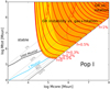 |
Fig. 4. Same as Fig. 3, but for the Pop I case (Tc = 8.5 × 10⁷ K). |
| In the text | |
|
Fig. 5. Internal profile of the dimensionless spin parameter at the limit of stability for f = 0.2%, Tc = 1.5 × 10⁸ K, and μ = 0.6, as a function of the mass-coordinate and for a choice of hylotropes with indicated φcore. The surface of each hylotrope is indicated by a white square. The black dashed curve shows the angular momentum accretion law (43). The red dashed curve and the red square indicate the limits for black hole formation, according to the criterions discussed in Sect. 4.3. |
| In the text | |
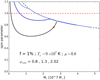 |
Fig. 6. Same as Fig. 5, but for f = 1% and Tc = 9 × 10⁷ K. |
| In the text | |
Current usage metrics show cumulative count of Article Views (full-text article views including HTML views, PDF and ePub downloads, according to the available data) and Abstracts Views on Vision4Press platform.
Data correspond to usage on the plateform after 2015. The current usage metrics is available 48-96 hours after online publication and is updated daily on week days.
Initial download of the metrics may take a while.