| Issue |
A&A
Volume 650, June 2021
|
|
|---|---|---|
| Article Number | A186 | |
| Number of page(s) | 14 | |
| Section | Numerical methods and codes | |
| DOI | https://doi.org/10.1051/0004-6361/202140624 | |
| Published online | 29 June 2021 | |
Two-body model for the spatial distribution of dust ejected from an atmosphereless body
Space Physics and Astronomy Research Unit, University of Oulu, Pentti Kaiteran katu 1, Oulu, Finland
e-mail: This email address is being protected from spambots. You need JavaScript enabled to view it.
; This email address is being protected from spambots. You need JavaScript enabled to view it.
Received:
22
February
2021
Accepted:
26
March
2021
Abstract
Aims. We present a model for the configuration of noninteracting material that is ejected in a continuous manner from an atmosphereless gravitating body for a given distribution of sources. The model is applicable to material on bound or unbound trajectories and to steady and nonsteady modes of ejection.
Methods. For a jet that is inclined to the surface normal, we related the distributions of ejection direction, velocity, and size to the phase-space number density at the distance from the source body. Integrating over velocity space, we obtained an expression from which we inferred the density, flux, or optical depth of the ejected material.
Results. As examples for the application of the code, we calculate profiles of the dust density in the Enceladus plume, the pattern of mass deposition rates around a plume on Europa, and images of optical depth following the nonstationary emission of material from a volcano on Io. We make the source code of a Fortran-95 implementation of the model freely available.
Key words: celestial mechanics / methods: analytical / methods: numerical
© ESO 2021
1. Introduction
The ejection of material from the surfaces of atmosphereless bodies is a ubiquitous phenomenon in the Solar System. Prominent examples are comets, active asteroids, ejecta clouds from hypervelocity impacts, or plumes from active satellites. For the dynamics of the ejected material, it is in many cases possible to neglect any other forces than the mass point gravity of the source body to a good degree of approximation. This is for instance the case for impact-generated dust clouds around planetary satellites as were detected around the Galilean moons (Krüger et al. 1999, 2003) or the Moon (Horányi et al. 2015), or dust plumes ejected from cryovolcanically active satellites (Spahn et al. 2006; Porco et al. 2006; Southworth et al. 2015). We note that for higher-order gravity terms to be negligible, the source body does not necessarily need to be spherical. For instance, mass-point gravity can be a good approximation to describe dust ejection from a satellite with surface topography.
In this paper we derive a semianalytical model to assess the spatial configuration of the emitted dust. The model relates the distribution of dust sources on the surface of the atmosphereless body and the parameters of ejection (e.g., source strength or directional and velocity distribution) to observable quantities such as number density, fluxes, or optical depth. The mathematical foundations are described in Sect. 2. Expanding on work in the literature (Krivov et al. 2003; Sremčević et al. 2003), our model can handle emission through inclined jets, and we develop a method for carrying out two of three integrations over the velocity distribution analytically. The code that implements the new model, carrying out the one remaining integration numerically, is called DUDI (for “dust distribution”) and is freely available under the GNU General Public License1. Aspects of the numerical algorithm for the integration are outlined in Sect. 3. Examples for an application of the model to current problems in planetary science are given in Sect. 4, including cases of steady and nonsteady dust emission.
2. Mathematical formulation
2.1. Phase-space density
We followed the derivations by Krivov et al. (2003), Sremčević et al. (2003), and Postberg et al. (2011) to relate the phase-space density of dust in a certain point of interest in space to the distributions that describe the ejection of the dust from a source on the moon surface. We generalized the existing model to allow emission from a point source in a direction that is not normal to the surface, with an axisymmetric distribution of ejection angles around this direction. Moreover, we allowed for a general coupling of the distribution of ejection velocities and grain size.
Our model was developed initially to fit in situ measurements by the Cassini Cosmic Dust Analyzer at the Saturn satellite Enceladus. For convenience, we use the words “spacecraft position” or “spacecraft coordinates” from now on to denote the point in space at which the dust density is calculated. We also use the term “density”, which at any point can be understood as the number density, mass density, the average radius of dust particles, or the cross section that is covered by the dust at the spacecraft position. The model allows us to obtain any of these quantities with a change of only one parameter.
We first consider a stationary process. We can equate the differential number of dust particles in a certain point of phase space
 (1)
(1)
to the number of particles ejected from the satellite surface
 (2)
(2)
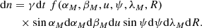
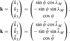
The variables used here are defined in Table 1, and Fig. 1 illustrates the geometry of the problem. For the phase-space density at the spacecraft, we obtain
 (3)
(3)
 |
Fig. 1. Directions to the north and to the positions of the source and the spacecraft form a spherical triangle. This establishes the relations between the angles of the problem. Here Δβ is the angle between the projections of vectors r and rM on the equatorial plane. |
Definition of variables.
For the two-body problem, the Jacobian can be obtained analytically (see Sremčević et al. 2003),
 (4)
(4)
We assume that the distribution function f factorizes, and that the distributions of the source position (fαM, βM), ejection speed (fu), ejection direction (fψ, λM), and size of the ejected dust particles (fR) can be defined separately,
 (5)
(5)
It is physically plausible that the distribution of the ejection speed of the dust particles depends on the grain size (Schmidt et al. 2008; Postberg et al. 2011), which we emphasize with the notation fu(u, R).
We describe the position of the point source located at the coordinates  on the surface of the spherical moon as the product of two Dirac δ-functions,
 (6)
(6)
The term sin αM in the denominator comes from the normalization.
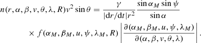
To formulate the directional distribution of ψ and λM so that it describes the ejection of dust that is axisymmetric around the axis of an inclined jet, we consider two coordinate systems centered at the location of the point source. The Z-axis of system (X, Y, Z) points along the local normal to the surface, and the X-axis points toward the local north. The  -axis of system
  is aligned with the axis of the jet. The axis
  lies on the line of nodes, so that the angle η* measured from X to
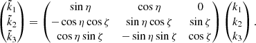
  is related to the jet azimuth η as η* = η − π/2. We define azimuth angles always clockwise from the local north, allowing a direct comparison to the derivations in Krivov et al. (2003) and Sremčević et al. (2003). Then, the transformation of the (X, Y, Z) coordinate system to the
  coordinate system may be performed as two subsequent rotations, as shown in Fig. 2. The first rotation is clockwise around the Z-axis with angle η*. The second rotation is counterclockwise around the
  -axis with angle ζ.
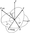 |
Fig. 2. Two coordinate systems centered at the location of the dust source on the surface of a spherical body. The Z-axis of system (X, Y, Z) is normal to the surface, and X points to the local north. The |


Let (ψ, λM) and  be the polar angle and azimuth in the two systems (X, Y, Z) and
  , respectively. The distribution of the ejection direction we wish to use can be formulated in a simple manner in terms of the variables
  because the distribution is symmetrical with respect to the axis
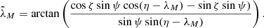
  . However, in Eq. (3) and in the formulae that are to be derived later in the course of solving the two-body problem, we have to deal with the angles (ψ, λM) that are defined in the local horizontal coordinate system. Therefore a replacement of the coordinates must be performed in the expression to obtain the distribution of ψ and λM, which can be used in further calculations. The desired function fψ, λM(ψ, λM) can be obtained by multiplication with the Jacobian,
 (7)
(7)
To express  and
and  through ψ and λM, we consider a unit vector k pointing in an arbitrary direction. In both coordinate systems the vector can be defined by Cartesian coordinates related to the corresponding polar coordinates as (we recall that λM and
  are azimuthal angles counted clockwise from the X and
  axes, respectively)
 (8)
(8)
The Cartesian coordinates of k in the two systems are related through the rotation matrix, which can be expressed in terms of η,
 (9)
(9)
Using Eqs. (8) and (9), we obtain
 (10)
(10)
 (11)
(11)
This gives the Jacobian
![Mathematical equation: $$ \begin{aligned}&\left|{\frac{\partial (\tilde{\psi }, \tilde{\lambda }_M)}{\partial (\psi , \lambda _M)}}\right|= 4\sin \psi \ / [10-2\cos 2\psi -3\cos 2(\psi - \zeta ) \nonumber \\&\qquad \qquad \ \ - 2\cos 2\zeta -3\cos 2(\psi + \zeta ) - 8\cos 2(\lambda _M-\eta )\sin ^2\zeta \sin ^2\psi \nonumber \\&\qquad \qquad \ \ -8\cos (\lambda _M-\eta )\sin 2\zeta \sin 2\psi ] ^{1/2}. \end{aligned} $$](/articles/aa/full_html/2021/06/aa40624-21/aa40624-21-eq29.gif) (12)
(12)
2.2. Integration
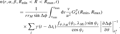
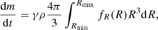
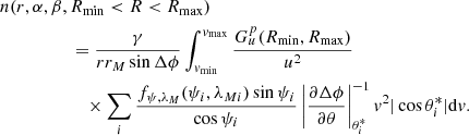
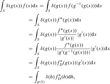
To compute the density of dust at the point (r, α, β), we must integrate Eq. (3) over all possible velocities and over all possible particle sizes,
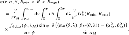 (13)
(13)
Here,
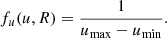
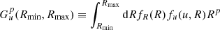 (14)
(14)
is defined in a similar way as in Postberg et al. (2011). The parameter p defines the moment of the size distribution related to the quantity we are interested in. Using p = 0, we obtain the number density of particles in the specified range of sizes. Setting p = 1 gives the average radius of the grains per unit volume. For p = 2 we obtain the average cross section of the dust particles per volume. This setting is used below to compute the geometrical optical depth of the dust population. Finally, p = 3 gives the average volume occupied by dust grains per unit volume. This setting is used to compute the mass density of the dust. For more details of the evaluation of  , see Appendix B. We replace variables in the argument of the δ function in Eq. (13) as
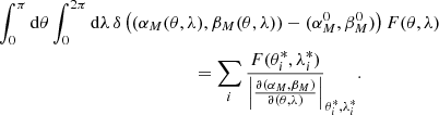 (15)
(15)
to integrate over θ and λ analytically. Equation (15) is derived in greater detail in Appendix A. Here, F(θ, λ) represents the integrand of Eq. (13), while θi and λi are the roots of the equation
 (16)
(16)
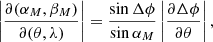
All the necessary dependencies between the variables in question can be found from spherical trigonometry (Krivov et al. 2003; Sremčević et al. 2003), for instance,
 (17)
(17)
and
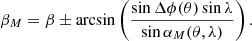 (18)
(18)
The spherical triangle used to obtain these relations is shown in Fig. 1. The angle Δϕ is the angle between the position vectors of the spacecraft and the source location on the moon. Because θ enters expressions (17) and (18) only through Δϕ, the partial derivatives of αM and βM with respect to θ can be computed as partial derivatives with respect to Δϕ multiplied by ∂Δϕ/∂θ. The Jacobian reads
 (19)
(19)
and our final formula is
 (20)
(20)
The integration over v must be carried out numerically. The lower integration limit is restricted by the minimum energy, or minimum semimajor axis, of the orbits that pass through the two points (rM, αM, βM) and (r, α, β). It is obtained from
 (21)
(21)
where
 (22)
(22)
The upper limit is constrained by the maximum ejection speed,
 (23)
(23)
The angle Δϕ in the expressions above is the angle between the position vector of the dust source, rM, and the position vector of the spacecraft, r. For a fixed position of the source and spacecraft, the angle Δϕ is also fixed, but it formally depends on v and θ. In the integrand of Eq. (20), the value v is given and Δϕ(θ) is a function of the variable θ alone. From the conservation equations of the two-body problem, we obtain
 (24)
(24)
 (25)
(25)
 (26)
(26)
 (27)
(27)
 (28)
(28)
which give the relation between Δϕ and θ. Following the notational convention of Krivov et al. (2003), we use dimensionless variables  and
and  , where vescape is the escape velocity on the satellite surface. The angles ϕ and ϕM are the true anomalies at r and rM, respectively.
Equations (24)–(28) can be used to calculate the partial derivative ∂Δϕ/∂θ. However, it is not possible to reverse these expressions to obtain θ from a given value of Δϕ analytically. The desired  are the values of θ that (for a given v) lead to a Δϕ satisfying Eqs. (17) and (18). We use a geometrical approach to calculate all possible
  . We consider the two-body problem, therefore the motion is restricted to a plane. We define a two-dimensional coordinate system in the plane containing the vectors r and rM. The origin is located at the moon center and r points along the x-axis. We know the lengths of r and rM as well as the angle Δϕ between them. Then the coordinates of the vectors r and rM in the plane are (r, 0) and (rMcos Δϕ, rMsin Δϕ).
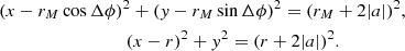
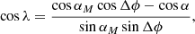
We wish to obtain θ, which is the angle between r and the grain velocity vector, which is tangential to the particle trajectory at the point r. This angle can be calculated when we know the equation of the trajectory, which is either an ellipse or a hyperbola. At this step (calculating the integrand of Eq. (20)), we know the value of the particle speed and the distance to the moon center, which determines the orbital energy, and thus, the semimajor axis a. We also know whether the particle moves along an ellipse (negative orbital engery) or along a hyperbola (positive orbital energy).
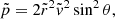
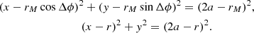
We first consider the case of an ellipse (Fig. 3). One of the focal points (F1) is located in the origin, which is the center of the moon. To draw the ellipse, we must find the position of the second focus. At each point of the ellipse, the sum of the distances to the focal points is a constant equal to 2a. Therefore the second focus must be removed from point r by 2a − r and from point rM by 2a − rM. These conditions are met at the intersection points of two circles centered at r and rM with radii 2a − r and 2a − rM, respectively.
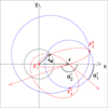 |
Fig. 3. Finding the second focus for an elliptic trajectory and the solutions for |

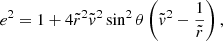
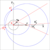 |
Fig. 4. Finding the second focus for an hyperbolic trajectory and the solutions for |


This leads to the conditions
 (29)
(29)
By solving the system of Eq. (29), we find two possible positions for the second focal point,  and
and  . In either case, we can calculate the eccentricity e of the ellipse, the true anomaly at point r, and, finally, the two solutions for θ using Eqs. (30)–(33). Knowing cos ϕM is sufficient to obtain ϕM because we know that the ejection point rM cannot have a true anomaly ϕM > π. We have
 (30)
(30)
 (31)
(31)
 (32)
(32)
 (33)
(33)
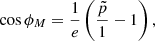
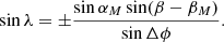
These equations determine the solutions  used in Eq. (20) if the particle travels from rM to r along the shorter arc of the ellipse. However, there are cases when a particle reaches r over an arc of 2π − Δϕ (Fig. 5), leaving rM in the opposite direction. To distinguish this case, we must recalculate r from the obtained value for ϕ using
 (34)
(34)
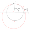 |
Fig. 5. Case when Δϕ should be replaced by 2π − Δϕ. |
and verify that it matches the starting value for r that we used to obtain ϕ. If this is not the case, then Δϕ in Eq. (32) must be replaced by 2π − Δϕ, which corresponds to the motion along the same ellipse, but in the opposite direction. This case is relatively rare, and in the examples we explored was only encountered at large distances from the source.
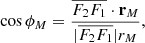
In case of hyperbolic motion (a < 0, Fig. 4), we follow almost the same line. For every point on a hyperbola, the difference between the distances to the focal points is the same. Because rM and r must be distances to the nearest focus, the system of equations for the coordinates of the second focal point reads
 (35)
(35)
Equations (30)–33 remain the same for the hyperbolic case. However, when the coordinates of the second focus are found, we must make sure that the particle does not pass the pericenter on its way from rM to r. For this purpose, we verify that the points rM and r lie on the same side of the line F1F2. If this condition is not satisfied, the solution is rejected. In Fig. 4 the hyperbola with second focus at the point  does not meet this condition. Therefore only one hyperbolic trajectory is possible to get from rM to r. Furthermore, the motion along the hyperbola is possible only in one direction. The value for sin ϕ is always positive and Δϕ = ϕ − ϕM.
The values of λi can be inferred from spherical trigonometry. The two solutions can be either identical or they differ by 180° because the motion is restricted to a plane,
 (36)
(36)
 (37)
(37)
The sign in Eq. (37) depends on the specific orientation of r and rM relative to the direction of zero-longitude. When the particle travels from rM to r over the angle of 2π − Δϕ, the signs of sin λ and cos λ both change because the sign of the sin Δϕ term in the denominator changes.
As soon as the values of  that satisfy the orbital geometry are known, they may be used to calculate the corresponding (u, ψi, λMi) from Eqs. (38)–(41) and the integrand in Eq. (20) is fully determined,
 (38)
(38)
 (39)
(39)
 (40)
(40)
 (41)
(41)
2.3. Nonstationary case
Nonstationary dust ejection can be modeled by allowing a time-dependent production rate γ in Eq. (20) that will result in a time-dependent spatial distribution of the dust. When we determine the orbital geometry for a fixed velocity value at the given point in space (Sect. 2.2), the time Δt required for traveling from rM to r along the Keplerian orbit can be calculated from Kepler’s equation. Thus, we know that the properties of the dust configuration at location r and time t are caused by the production of dust at the source location rM with the rate γ(t − Δt). In this case, the production rate cannot be put outside the integral and Eq. (20) becomes
 (42)
(42)
The two solutions for Δti follow from Kepler’s equation using the two solutions for eccentricity from Eq. (30) and computing the eccentric anomaly with the half-angle formula from the true anomaly given by Eq. (32).
2.4. Singularities of the coordinates
There are coordinates for which solutions of Eqs. (20) or (42) cannot be obtained (see Table 2). The problem arises from the use of a spherical coordinate system. In practice, it is possible to avoid the singularities by carefully choosing the pole axis of the coordinate system after the source location and the detector position of interest are known. If coordinates close to the singularities need to be evaluated, then the stability and accuracy of the numerical integration becomes a challenge. However, double-precision calculations allow approaching the singular angles as close as 10−4 radians. This difference from the values listed in Table 2 can be considered safe, and with a possible moderate loss of accuracy, the model can be applied within an even closer vicinity of the singularities.
Coordinate singularities of the model.
3. Numerical integration
In this section we present and discuss the algorithm for the numerical solution of Eqs. (20) and (42). We have implemented this algorithm in a code written in Fortran-95, which we call dust distribution (DUDI). The source code with technical documentation and instructions for usage and compilation is freely available under the GNU General Public License2. The makefile provided for compilation uses the gfortran compiler. DUDI can be compiled and run without installing additional libraries. The library of OpenMP, which is used to speed the computation up, is included in the compiler.
DUDI allows us to compute the number density of dust or related quantities at given points in space as a mean radius, average cross section, or mass density of the dust grains ejected from the surface of a spherical body without an atmosphere. The input data are the spacecraft coordinates, the properties of the source (i.e., the location and the distributions of the direction and speed of the ejection) and the three parameters of  .
.
The first preliminary step is to calculate  on a grid of u-values. The array of pairs
  is later used to interpolate
  for the actually required value u under the integrand of Eqs. (20) or (42). The second preliminary step is to compute the values of Δϕ and Δβ for the given positions of the source and the spacecraft.
Then we proceed directly to the numerical evaluation of the integral over velocity in Eq. (20) in the stationary case, or Eq. (42) if there is a time-dependence. The ejection speed distribution implies a certain lower limit for the possible ejection speed umin. At any point r, this minimum ejection velocity restricts the corresponding minimum velocity at spacecraft position  , which may be higher than the lower integration limit given by Eqs. (21)–(22). The actual numerical integration is performed over the interval where (vmin, vmax) and
  overlap. The minimum and maximum ejection speed umin and umax (in m s−1) must be explicitly specified as a property of the dust source, along with the expression for the ejection speed distribution.
At each step of the integration, we find for a given v, r, and Δϕ the solutions for the angles θ and λ as described in Sect. 2.2. We control the accuracy of the solution for θ by recalculating the value of Δϕ from Eqs. (24)–(28) and comparing it to the starting value of Δϕ as given by the positions of the dust source and the spacecraft. We require the difference between the two values of Δϕ to be smaller than 10−4Δϕ. In most cases the accuracy is much better, but it may degrade for certain values of v near the singularities of the coordinates (see Sect. 2.4) or when r ≈ rM. Even for poor accuracy for θ, this means that the accuracy decreases only for one or two integration steps. The error in the final result is smaller. We consider the relative accuracy of 10−4 sufficient for the θ solutions. If it is worse, a warning is produced by the program.
We divide the integration domain into two regions as (vmin, vpar) and (vpar, vmax) to obtain the number density of the particles on elliptic and hyperbolic (escaping) trajectories separately. Here vpar (the subscript stands for “parabolic”) is the minimum escape velocity at radial distance r.
When  , the integrand in Eq. (20) has a pole at v = vmin. We replace vmin from Eq. (21) with vmin + Δ, where Δ = 10−10 has turned out to be a good choice to evaluate the integrand near the pole to reasonable accuracy in a stable manner. To better resolve the pole, we additionally subdivide the elliptic part of the integral into two parts that are treated separately. The first integration subinterval is (vmin, v1), where
  is the domain that contains the pole. Here integration is performed using the trapezoidal rule with a large number of supports that become denser toward vmin as
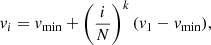 (43)
(43)
where N is the number of supports. Then we use the Gauss-Legendre quadrature of a moderate order to compute the integral from v1 to vpar. The integration over the hyperbolic velocities is also performed with a Gauss-Legendre quadrature. The choice of the quadrature order depends on the integration domain and ejection speed distribution. The nodes and weights of the Gauss-Legendre formula are tabulated in our code for the following orders: 5, 10, 20, 30, 40, and 50.
Figures 6–9 show examples for the behavior of the integrand in the three domains. Depending on the choice of the ejection speed distribution fu(u, R), the integrand may decrease (Fig. 7) or increase (Fig. 8) toward higher velocities. Remarkably, the integrand can jump at v = vpar (Fig. 9) if a significant part of the dust number density is due to the particles on their way back to the moon after passage of their apocenter,
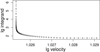 |
Fig. 6. Pole at v = vmin. |
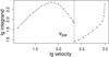 |
Fig. 9. Integrand from Eq. (20). A high abundance of dust falling back causes a jump at the transition from the elliptic to the hyperbolic case. |
The sharpness of the pole varies. At each integration step, the given velocity v determines the values of θ that enter the integrand of Eq. (20) through the derivative ∂Δϕ/∂θ and ψ(θ). The latter is needed to compute the ejection angle distribution fψ, λM(ψ, λM). The factor ∂Δϕ/∂θ is the reason for the pole. Its value depends on θ and on the spacecraft position relative to the source. The pole is less strongly peaked if the value of ψ(θ) corresponds to a very unlikely ejection direction. Thus, the sharpness of the pole depends on the spacecraft position relative to the source position and also on the ejection angle distribution, and so does the number of integration steps required to achieve a given accuracy goal.
The accuracy can be estimated from Eq. (44), where P is the value of the pole integral (between vmin and v1) obtained with N steps for the integration with the trapezoidal rule, and Nmax is the maximum reasonable number of steps. Nmax is limited by accumulated rounding errors, and we determine its value in test integrations. I(Nmax) is the sum of P(Nmax) and the remaining part of the integral between v1 and vmax. In this way, we can quantify the discrepancy induced by the pole integration in the final result,
 (44)
(44)
We require ϵ ≤ 10−3 and perform tests to determine the corresponding number of pole integration steps N necessary to achieve this goal. This number we compute for different spacecraft positions relative to the source and to the axis of ejection symmetry (the polar angle in the coordinate system  in Fig. 2, in the following denoted by ξ). We adopt
 (45)
(45)
for the ejection direction distribution. Normalization in this expression does not matter for an evaluation of ϵ from Eq. (44). We vary the parameters ψmax and ω, along with the polar angle of the ejection symmetry axis, to investigate the behavior of the pole for different ejection distributions, of which two main classes can be defined. The “jets” are the sources with a preferred direction of ejection, and the “diffuse sources” have no such direction. We find that for diffuse ejection (ω = 45° and ψmax = 45°), N = 15 is a sufficient number of supports to achieve ϵ ≤ 10−3 at any spacecraft position. For a vertical jet (ψmax = 0° and ω in the range of 3° and 5°), the value of P can be neglected for all ξ > 40° and N = 15 is sufficient for ξ < 40°.
However, for a narrow and inclined jet, we find that there are points where a large number of supports is required to integrate the pole accurately. The narrower and the more inclined the jet, the greater the number of these points and the greater the required N. We focus on the worst-case scenarios generally to constrain an optimal number of steps required for the pole integration.
Empirically, we find that an accuracy of 10−3 can be achieved with a minimum number of steps when an exponent of k = 4 is used in Eq. (43). Figures 10 and 11 show examples of how the minimum number of steps required to integrate the pole with the given accuracy is distributed over r and ξ values. N = 0 means that the pole does not have to be integrated at all because its value is negligible.
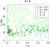 |
Fig. 10. Minimum number of supports necessary to achieve an accuracy of 10−3 (Eq. (44)) in the integration of the pole of the integrand (Fig. 6) for the case of a narrow jet (ω = 3° , ψmax = 0°), tilted by z = 20° . |
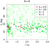 |
Fig. 11. Minimum number of supports necessary to achieve an accuracy of 10−3 (Eq. (44)) in the integration of the pole of the integrand (Fig. 6) for the case of a narrow jet (ω = 3° , ψmax = 0°), tilted by z = 30° . |
For jets, we select the number of supports N for the pole integration based on the distributions shown in Figs. 10 and 11 as follows:
![Mathematical equation: $$ \begin{aligned} N = \!\left\{ \begin{array}{cl} 0,&\! \xi > 45^\circ \ \mathrm{or} \ \,\xi < 10^\circ ,\ r/r_M > 1.05,\\ 80,&\! \xi > 45^\circ \ \mathrm{or} \ \,\xi < 10^\circ ,\ r/r_M < 1.05,\\ 15 + 10z[\mathrm{deg} ],&\!10^\circ < \xi < 45^\circ , \ r/r_M <2,\\ 10 + 5z[\mathrm{deg} ],&\!10^\circ < \xi < 45^\circ , \ r/r_M >2.\\ \end{array}\right. \end{aligned} $$](/articles/aa/full_html/2021/06/aa40624-21/aa40624-21-eq85.gif) (46)
(46)
4. Applications
In this section we present three applications of the model to phenomena of scientific interest in the Solar System. The purpose of these examples is to demonstrate the wide range of applicability of the model. We leave a rigorous scientific analysis of these problems with a comprehensive comparison to data for future work.
4.1. Density profile of the Enceladus dust plume
On July 14, 2005, the Cassini spacecraft performed a flyby at the Saturnian moon Enceladus (labeled E2). During the flyby, the High Rate Detector (HRD), a subsystem of the Cassini Cosmic Dust Analyzer instrument (Srama et al. 2004), measured the number density of dust particles in the vicinity of the satellite. The significant increase in dust density near Enceladus (see Fig. 12), about one minute prior to the closest approach of the spacecraft to the satellite, was the first in situ measurement of particles in the Enceladus dust plume (Spahn et al. 2006). Dust and vapor are emitted from four fissures called the tiger stripes in the anomalously warm south polar terrain of Enceladus (Spencer et al. 2006; Porco et al. 2006). A part of this dust escapes the moon gravity and forms the dusty E ring of Saturn (Horányi et al. 2009; Kempf et al. 2018).
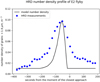 |
Fig. 12. Dust number density profile observed by the HRD during the E2 flyby of the Cassini spacecraft at Enceladus and results from modeling the emission from one single jet in the south polar terrain (see text for details). |
From an analysis of high phase-angle images, Porco et al. (2014) suggested a list of 100 jets of dust emission for which the coordinates and tilts were derived from images (see also Spitale et al. 2015). To demonstrate an application of our model to the dust emission from Enceladus, we selected one single jet from this list with coordinates (−80.25° N, 55.23° E), which is tilted by 5° from the surface normal in an azimuthal direction 38° away from local north. The ejection is stationary, so that the production rate γ(t) is constant. The distributions we implemented for particle sizes, ejection speed, and direction are given by
 (47)
(47)
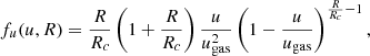 (48)
(48)
and
 (49)
(49)
Equation (48) was derived by Schmidt et al. (2008) to describe the acceleration of dust grains in the gas flux in the vents that supply the sources. Particles smaller than Rc (measured in the same units as R) tend to accelerate up to the gas velocity (ugas), while particles larger than Rc are significantly slower. For this distribution, we have umin = 0, while umax is equal to the gas velocity ugas. Table 3 lists the parameters of the distributions and other parameters that are necessary to set up the model. Figure 12 shows the result for the number density of dust obtained from the model for the single jet, evaluated along the trajectory of Cassini during the E2 flyby. The model was evaluated for grains with a radius larger that 1.6 micron, which corresponds to the size threshold for the HRD data shown in the plot. We multiplied the model profile by a factor so that the peak matches the measured peak density. To match the HRD profile at a large distance from the plume, we added a constant background of 0.01 particles/m3 to the model number density. The selection of the grain size in the model was realized by adjusting the function  appropriately (see Table 3). We obtained the position of the spacecraft from the reconstructed spice kernels of the mission3, using the NAIF Spice toolkit4. Using these parameters, we recovered the location of the maximum number density on the Cassini trajectory (Fig. 12). Our model could now be applied to all the jets identified by Porco et al. (2014), and the results could be fit to in situ data. Similarly, we could calculate the geometrical optical depths of the dust emitted along a given line of sight and compare this to the brightness distribution in images (see Sect. 4.3 for an example). For a quantitative comparison to images, we can apply light scattering modeling to the dust configuration that is derived from the dust distribution model.
Parameters used to model the number density profile of the E2 flyby.
4.2. Surface deposition of material from plumes on Europa
There is evidence that cryovolcanic activity also generates plumes on the Jupiter satellite Europa (Fagents et al. 2000; Phillips et al. 2000; Roth et al. 2014; Sparks et al. 2016; Jia et al. 2018). Owing to the higher gravity of Europa, plumes would be more confined than those on Enceladus, and they may be harder to observe or sample directly (Southworth et al. 2015; Quick & Hedman 2020). However, surface features from plume deposits may provide evidence for past cryovolcanic activity, and if spectral features exist, allow the remote characterization of material from the interior (Fagents et al. 2000; Phillips et al. 2000; Quick & Hedman 2020).
We calculated the radial variation of the mass flux of dust grains falling back onto the surface, considering four different dust sources with identical characteristics except for the particle size distribution and the distribution of ejection directions. We considered two size distributions and two ejection modes: one describing a narrow jet, and the other describing a broader, more diffuse ejection. For the size distributions we employed a power law
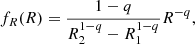 (50)
(50)
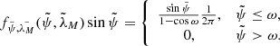
with two different values of the exponent q. The greater q, the more abundant the small dust particles. For the ejection direction, we used a pseudo-Gaussian distribution of the polar angle
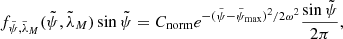 (51)
(51)
giving a nonzero probability of ejection in any direction. The normalization constant Cnorm was found numerically for fixed values of ψmax and ω. The dust production rate γ was identical for all the sources, meaning that they produced the same number of dust particles per unit time, but we then obtained different mass production rates for the different size distributions. For the ejection speed distribution we again used Eq. (48). Table 4 lists the distribution parameters.
Parameters used to model the radial distribution of dust deposition on the surface of Europa.
We can compute the rate of dust mass produced per second from the size distribution as
 (52)
(52)
where ρ is the density of the ice grains, and the grains were assumed to be spherical.
To compute flux instead of density, we must modify Eq. (20) as
 (53)
(53)
As the vector r is normal to the surface of the satellite, the factor v|cos θ| turns the density into the flux of dust falling back to the moon. Multiplying equation Eq. (53) by 4πρ/3 (ρ is the density of the particle material) and setting p = 3 and r = rM gives the mass flux onto the surface. Because r = rM on the surface, it is geometrically impossible to obtain  or any particles moving upward.
With the parameters from Table 4, Eq. (52) gives 0.6 kg of dust produced each second for the source with the shallow size distribution (q = 3) and 0.05 kg for the source with the steep size distribution (q = 5). Figure 13 shows the distribution of the dust deposition (mass flux onto the surface) with distance from the source on the moon surface.
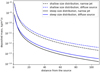 |
Fig. 13. Dust flux on the surface of the moon at various distances from the dust source. The production rate of the sources with shallow dust size distribution is 0.6 kg s−1, and the production rate of the sources with steep size distribution is 0.05 kg s−1. |
Taking the observational evidence together, we expect the outgassing activity on Europa to be intermittent or episodic, with a potentially complex time dependence. This case could be modeled using a time-dependent function for the dust production rate. We consider a time-dependent dust ejection in our final example.
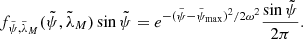
4.3. Images of a volcanic eruption on Io
The innermost satellite of Jupiter, Io, is a geologically very active body. It has multiple volcanic centers scattered over its surface (Strom et al. 1979; Keszthelyi et al. 2001; Geissler et al. 2004). The volcanic plumes vary in many features as shape, size and period of activity and often they are asymmetric. Our model allows to investigate such plumes by using inclined jets with time-dependent eruptions, or even a simultaneous dust ejection from sources with different properties.
The main flaw of our model in application to the Io volcanic plumes is that the gas emerging from the vents is generally not collisionless. In the dense cores of the plumes, condensation occurs up to a height of several hundred kilometers (Cataldo et al. 2002). Moreover, the dynamics of the dust will be influenced by the surrounding gas. Condensation (i.e., dust production) in the plume might be taken into account in principle by modeling such a plume with additional point sources placed within the condensation column, with appropriately adjusted time-dependent dust production rates. For this purpose, we implemented in the code the possibility of computing the dust density also at locations below (closer to the moon center) the location of the source. In this case, we still use the assumption that the true anomaly at the location of the source is lower than π, that is, downward ejection from a source located above the surface is not possible.
In our simple example presented here, we considered just one source located on the surface to represent a volcanic plume with a finite duration of activity. We took several images of the expanding dust plume from the same point in space with a favorable geometry when the volcano is located at the limb of the moon. We also assumed that the glow of the surface of Io was already subtracted from the images but a homogeneous background brightness was present, so that the moon disk looks dark against this background. We tilted the volcano slightly by 3° toward local south. The volcano was not exactly in the center of the image for the purpose of reducing the computational difficulties arising when Δϕ or Δβ ≈ 0 (see Sect. 2.4).
Synthetic images of size 128x128 pixels were then constructed in the following way. Each pixel corresponds to a line of sight. We placed a grid of points on the line of sight for which we calculated the total cross section covered by the dust grains (p = 2 in Eq. (14)). Then we integrated over the lines of sight to obtain the geometrical optical depth (total particle cross section per area covered by the pixel). The color of a pixel then corresponded to the value determined for the geometric optical depth.
We employed Eq. (50) for the size distribution, Eq. (51) for the distribution of the ejection direction, and a simple size-independent expression (Eq. (54)) for a uniform ejection speed distribution,
 (54)
(54)
When the time interval in which the plume is observed is much shorter than the characteristic time of the plume variability, the ejection can be considered steady. However, here we modeled a nonstationary volcanic plume that was active for only 1000 seconds and constructed nine snapshots of this plume to show the evolution of the space distribution of dust with time
 (55)
(55)
where tmax = 500 s. Table 5 describes the model setup, and the images are shown in Fig. 14
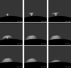 |
Fig. 14. Images of a fictive volcanic plume on Io taken at different stages of eruption. |
Parameters used to construct the volcanic plume images.
Compared to the examples from Sects. 4.1 and 4.2, the construction of images is computationally expensive. Therefore it makes sense to avoid calculations of the properties in those points where the value would not affect the final result. In the case considered here, the maximum ejection velocity was set to be lower than the escape velocity of Io, so that there is a maximum height that the particles can reach. Moreover, the disk of the moon covers part of the images. Taking these two facts into account, we excluded the points on the lines of sight from the calculations that crossed the moon disk and the points that lie at a greater distance from the surface than the maximum height.
5. Discussion
We developed a semianalytical model that allows the user to derive the average properties of dust (number or mass density, fluxes, and optical depths) ejected from an atmosphereless body. Physically, our approach is based on the two-body problem, that is, it neglects any forces on the dust particles other than the point-mass gravity of the source body. We show that the model still has a wide range of applications. These are situations where the gravity of other perturbing bodies and higher-order gravity from a nonspherical mass distribution of the central body can be neglected along the entire path that a dust particle takes from its source to its sink. The nongravitational forces must also be negligibly small, for instance, electromagnetic forces acting on charged grains, radiation-induced forces (solar radiation pressure and Poynting-Robertson drag), and drag exerted by ambient gas or plasma. For instance, the model can be applied to the Enceladus dust plume in a region that is sufficiently close to the dust sources on the south polar terrain of this satellite. It cannot be applied to estimate the dust density at higher northern latitudes of Enceladus, however, because this region is too far away from the sources near the south pole, and three-body forces due to Saturn have already affected the shape of the dust configuration. This can be seen in a peculiar pattern of color variation Schenk et al. (2011a), that can be matched with two wedge shaped regions extending deep into the northern hemisphere (Schenk et al. 2011b, 2017), for which three body models of the plume predict enhanced fall back rates of south polar dust (Kempf et al. 2010). The model can be applied to investigate the dust clouds around the Galilean moons (Krüger et al. 1999) at any longitude and latitude, however, because in this case, the dust emission occurs (nearly) uniformly over the whole surface of the satellites as long as the point of interest is located deeply enough in the Hill sphere of the satellite.
Mathematically, our model relates the dust distribution at the site of ejection to the distribution at the point of interest (spacecraft position) by using the conservation laws of energy and momentum provided by the two-body problem (Krivov et al. 2003; Sremčević et al. 2003). We use the fact that the position of the spacecraft, the position of the source, and the center of the moon define the plane to which the movement is restricted. In the evaluation of the dust properties at a given point, this allows us to carry out two of the three integrations over velocity space analytically. Only one remaining integration must then be performed numerically. The distribution-based approach is very flexible, and because it allows employing asymmetric and nonstationary modes of dust emission, it allows modeling quite complex situations. A time dependence could relatively easily be introduced in the distributions of ejection speed, direction, and size as well. Furthermore, the model could also be extended to model dust emission from a comet or an active asteroid, making the Sun the central body and using a rescaled solar mass to account for the radiation pressure.
Relying only on one numerical integration, the model becomes computationally very efficient, so that even image reconstruction becomes feasible, although it involves the evaluation of the dust properties in the three-dimensional region that is in the field of view. From the examples discussed in Sect. 4, the image of the volcano (Sect. 4.3) is the most computationally demanding. Nevertheless, on a usual four-core PC, each image in Fig. 14 required 0.4 s of elapsed time to be obtained.
The model is implemented in Fortran-95, and the package called DUDI is available5 for free usage under the terms of GNU General Public License. A user can use the probability density functions and choose from several variants that are already implemented in the described examples, or they can implement new variants.
Acknowledgments
This work was supported by the Academy of Finland.
References
- Cataldo, E., Wilson, L., Lane, S., & Gilbert, J. 2002, J. Geophys. Res., 107, E11 [CrossRef] [Google Scholar]
- Fagents, S. A., Greeley, R., Sullivan, R. J., et al. 2000, Icarus, 144, 54 [CrossRef] [Google Scholar]
- Geissler, P., McEwen, A., Phillips, C., Keszthelyi, L., & Spencer, J. R. 2004, Icarus, 169, 29 [NASA ADS] [CrossRef] [Google Scholar]
- Gelfand, I. M., & Shilov, G. E. 1968, Generalized Functions, 1 (Academic press) [Google Scholar]
- Horányi, M., Burns, J. A., Hedman, M. M., Jones, G. H., & Kempf, S. 2009, Diffuse Rings, 511, [Google Scholar]
- Horányi, M., Szalay, J. R., Kempf, S., et al. 2015, Nature, 522, 324 [NASA ADS] [CrossRef] [Google Scholar]
- Jia, X., Kivelson, M. G., Khurana, K. K., & Kurth, W. S. 2018, Nat. Astron., 395, 1 [Google Scholar]
- Kempf, S., Beckmann, U., & Schmidt, J. 2010, Icarus, 206, 446 [CrossRef] [Google Scholar]
- Kempf, S., Horányi, M., Hsu, H. W., et al. 2018, Saturn’s Diffuse E Ring and Its Connection with Enceladus, 195 [Google Scholar]
- Keszthelyi, L., McEwen, A., Phillips, C., et al. 2001, J. Geophys. Res, 106, 33025 [CrossRef] [Google Scholar]
- Krivov, A. V., Sremčević, M., Spahn, F., Dikarev, V., & Kholshevnikov, K. V. 2003, Planet. Space Sci., 51, 251 [NASA ADS] [CrossRef] [Google Scholar]
- Krüger, H., Krivov, A. V., Hamilton, D. P., & Grün, E. 1999, Nature, 399, 558 [NASA ADS] [CrossRef] [Google Scholar]
- Krüger, H., Krivov, A. V., Sremčević, M., & Grün, E. 2003, Icarus, 164, 170 [NASA ADS] [CrossRef] [Google Scholar]
- Phillips, C. B., McEwen, A. S., Hoppa, G. V., et al. 2000, J. Geophys. Res., 105, 22579 [CrossRef] [Google Scholar]
- Porco, C. C., Helfenstein, P., Thomas, P. C., et al. 2006, Science, 311, 1393 [Google Scholar]
- Porco, C., DiNino, D., & Nimmo, F. 2014, AJ, 148, 45 [CrossRef] [Google Scholar]
- Postberg, F., Schmidt, J., Hillier, J. K., Kempf, S., & Srama, R. 2011, Nature, 474, 620 [NASA ADS] [CrossRef] [Google Scholar]
- Quick, L. C., & Hedman, M. M. 2020, Icarus, 343, 113667 [CrossRef] [Google Scholar]
- Roth, L., Saur, J., Retherford, K. D., et al. 2014, Science, 343, 171 [NASA ADS] [CrossRef] [Google Scholar]
- Schenk, P., Hamilton, D. P., Johnson, R. E., et al. 2011a, Icarus, 211, 740 [NASA ADS] [CrossRef] [Google Scholar]
- Schenk, P., Schmidt, J., & White, O. 2011b, EPSC-DPS Joint Meeting 2011, 2-7 October 2011, Nantes, France, http://meetings.copernicus.org/epsc-dps2011, 1358 [Google Scholar]
- Schenk, P., Buratti, B., Helfenstein, P., Kempf, S., & Schmidt, J. 2017, 48th Lunar Planet. Sci. Conf., Woodlands, Texas, LPI Contribution No. 1964, 2601 [Google Scholar]
- Schmidt, J., Brilliantov, N. V., Spahn, F., & Kempf, S. 2008, Nature, 451, 685 [CrossRef] [PubMed] [Google Scholar]
- Southworth, B. S., Kempf, S., & Schmidt, J. 2015, Geophys. Res. Lett., 42, 10 [CrossRef] [Google Scholar]
- Spahn, F., Schmidt, J., Albers, N., et al. 2006, Science, 311, 1416 [NASA ADS] [CrossRef] [Google Scholar]
- Sparks, W. B., Hand, K. P., McGrath, M. A., et al. 2016, ApJ, 829, 1 [NASA ADS] [CrossRef] [Google Scholar]
- Spencer, J. R., Pearl, J. C., Segura, M., et al. 2006, Science, 311, 1401 [NASA ADS] [CrossRef] [PubMed] [Google Scholar]
- Spitale, J. N., Hurford, T. A., Rhoden, A. R., Berkson, E. E., & Platts, S. S. 2015, Nature, 521, 57 [NASA ADS] [CrossRef] [Google Scholar]
- Srama, R., Ahrens, T., Altobelli, N., et al. 2004, Space Sci. Rev., 114, 465 [NASA ADS] [CrossRef] [Google Scholar]
- Sremčević, M., Krivov, A. V., & Spahn, F. 2003, Planet. Space Sci., 51, 455 [CrossRef] [Google Scholar]
- Strom, R. G., Terrile, J. R., Masursky, H., & Hansen, C. 1979, Nature, 280, 733 [CrossRef] [Google Scholar]
Appendix A: Replacement of the variable in the argument of Dirac’s δ-function
Let x ∈ S ⊂ ℝn; f, g : S → ℝn. Then we can perform a replacement of the variable under the integral based on Eqs. (A.1) and (A.2) from Gelfand & Shilov (1968),
 (A.1)
(A.1)
Here, g′ is the Jacobian matrix of the function g, |g′| denotes the Jacobi determinant, and xi are the zeros of g,
 (A.2)
(A.2)
where
Upon integration, we obtain
In our case, n = 2, the function g performs a transformation from (αM, βM) to (θ, λ), and the function f represents all the dependences on θ and λ in the integrand in Eq. (13).
Appendix B: Physical meaning of the function Gu
For each source, the first step in the numerical calculations is to obtain values of  (Eq. (14)) on a dense grid of u. This means that we perform integrations over the particle size R treating u as a parameter. The size distribution fR(R) can be defined on an interval of grain sizes, its lower and upper boundaries being parameters of the distribution.
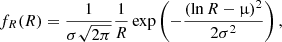
These boundaries need not necessarily be equal to Rmin and Rmax. Instead, Rmin and Rmax should be understood as limits of an observable interval of particle radii. Particles smaller than Rmin or larger than Rmax may exist, and they contribute to the normalization of fR(R), but they would not contribute to the value of n (Eq. (20)). This concept is illustrated in Figs. B.1 and B.2. The quantity plotted in the two figures is fR(R)fu(u, R). In Fig. B.1, fR(R) is a lognormal distribution that is formally defined in the interval (0, +∞), or in other words,  , and the interval (Rmin, Rmax) does not cover the whole domain of fR(R). In Fig. B.2, the particle sizes are distributed between certain R1 and R2 as Eq. (50). In this example, Rmin = R1, but Rmax < R2. If Rmin were lower than R1, it would not have changed the result because for R < R1, we have fR(R) = 0.
Although we defined the size distribution outside the interval (Rmin, Rmax), its shape there does not affect the final result as long as it remains the same inside (Rmin, Rmax). However, we can investigate the defined size distribution by applying different values of Rmin and Rmax. This approach implies that the size distribution and the initial speed distribution are physical characteristics of the dust source, while Rmin and Rmax represent the sensitivity range of the instrument with which we perform observations. In the model implementation DUDI, the interval (Rmin, Rmax) can coincide with the fR(R) domain or can be even larger.
The units of the particle radius R matter only in the definition of fR and fu, so that we suggest measuring R in microns to have simpler numbers in the expressions. With different formulae for fR and fu, shorter expressions for  can be obtained that require less cumbersome computations (see, e.g., Postberg et al. 2011). However, we purposefully consider a set of fR and fu in our model that cannot be simplified to show the general form of the solution and to allow flexibility in applying the model.
All Tables
Parameters used to model the radial distribution of dust deposition on the surface of Europa.
All Figures
|
Fig. 1. Directions to the north and to the positions of the source and the spacecraft form a spherical triangle. This establishes the relations between the angles of the problem. Here Δβ is the angle between the projections of vectors r and rM on the equatorial plane. |
| In the text | |
|
Fig. 2. Two coordinate systems centered at the location of the dust source on the surface of a spherical body. The Z-axis of system (X, Y, Z) is normal to the surface, and X points to the local north. The |
| In the text | |
|
Fig. 3. Finding the second focus for an elliptic trajectory and the solutions for |
| In the text | |
|
Fig. 4. Finding the second focus for an hyperbolic trajectory and the solutions for |
| In the text | |
|
Fig. 5. Case when Δϕ should be replaced by 2π − Δϕ. |
| In the text | |
|
Fig. 6. Pole at v = vmin. |
| In the text | |
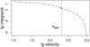 |
Fig. 7. Integrand from Eq. (20) for an ejection speed distribution that favors low velocities. |
| In the text | |
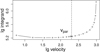 |
Fig. 8. Integrand from Eq. (20) for an ejection speed distribution that favors high velocities. |
| In the text | |
|
Fig. 9. Integrand from Eq. (20). A high abundance of dust falling back causes a jump at the transition from the elliptic to the hyperbolic case. |
| In the text | |
|
Fig. 10. Minimum number of supports necessary to achieve an accuracy of 10−3 (Eq. (44)) in the integration of the pole of the integrand (Fig. 6) for the case of a narrow jet (ω = 3° , ψmax = 0°), tilted by z = 20° . |
| In the text | |
|
Fig. 11. Minimum number of supports necessary to achieve an accuracy of 10−3 (Eq. (44)) in the integration of the pole of the integrand (Fig. 6) for the case of a narrow jet (ω = 3° , ψmax = 0°), tilted by z = 30° . |
| In the text | |
|
Fig. 12. Dust number density profile observed by the HRD during the E2 flyby of the Cassini spacecraft at Enceladus and results from modeling the emission from one single jet in the south polar terrain (see text for details). |
| In the text | |
|
Fig. 13. Dust flux on the surface of the moon at various distances from the dust source. The production rate of the sources with shallow dust size distribution is 0.6 kg s−1, and the production rate of the sources with steep size distribution is 0.05 kg s−1. |
| In the text | |
|
Fig. 14. Images of a fictive volcanic plume on Io taken at different stages of eruption. |
| In the text | |
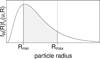 |
Fig. B.1. Integrand in Eq. (14) with a lognormal size distribution and a fixed value of u. |
| In the text | |
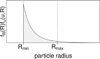 |
Fig. B.2. Integrand in Eq. (14) with a power-law size distribution and a fixed value of u. |
| In the text | |
Current usage metrics show cumulative count of Article Views (full-text article views including HTML views, PDF and ePub downloads, according to the available data) and Abstracts Views on Vision4Press platform.
Data correspond to usage on the plateform after 2015. The current usage metrics is available 48-96 hours after online publication and is updated daily on week days.
Initial download of the metrics may take a while.