| Issue |
A&A
Volume 650, June 2021
|
|
|---|---|---|
| Article Number | A144 | |
| Number of page(s) | 14 | |
| Section | The Sun and the Heliosphere | |
| DOI | https://doi.org/10.1051/0004-6361/202140534 | |
| Published online | 22 June 2021 | |
Stability of solar atmospheric structures harboring standing slow waves
An analytical model in a compressible plasma
Centre for mathematical Plasma Astrophysics (CmPA), Mathematics Department, KU Leuven, Celestijnenlaan 200B Bus 2400, 3001 Leuven, Belgium
e-mail: michael.geeraerts@kuleuven.be
Received:
11
February
2021
Accepted:
26
April
2021
Context. In the context of the solar coronal heating problem, one possible explanation for the high coronal temperature is the release of energy by magnetohydrodynamic (MHD) waves. The energy transfer is believed to be possible, among others, by the development of the Kelvin-Helmholtz instability (KHI) in coronal loops.
Aims. Our aim is to determine if standing slow waves in solar atmospheric structures such as coronal loops, and also prominence threads, sunspots, and pores, can trigger the KHI due to the oscillating shear flow at the structure’s boundary.
Methods. We used linearized nonstationary MHD to work out an analytical model in a cartesian reference frame. The model describes a compressible plasma near a discontinuous interface separating two regions of homogeneous plasma, each harboring an oscillating velocity field with a constant amplitude which is parallel to the background magnetic field and aligned with the interface. The obtained analytical results were then used to determine the stability of said interface, both in coronal and photospheric conditions.
Results. We find that the stability of the interface is determined by a Mathieu equation. In function of the parameters of this equation, the interface can either be stable or unstable. For coronal as well as photospheric conditions, we find that the interface is stable with respect to the KHI. Theoretically, it can, however, be unstable with respect to a parametric resonance instability, although it seems physically unlikely. We conclude that, in this simplified setup, a standing slow wave does not trigger the KHI without the involvement of additional physical processes.
Key words: Sun: corona / magnetohydrodynamics (MHD) / plasmas / waves / instabilities
© ESO 2021
1. Introduction
Although it has been known for a long time that the corona is three orders of magnitude hotter than the photosphere, a definite explanation for this unexpected feature has continued to elude researchers. One possible explanation that has been advanced over the years, and which is supported by both observations and theoretical models, is the deposition of energy of magnetohydrodynamic (MHD) waves into the corona (Parnell & De Moortel 2012; Arregui 2015; Van Doorsselaere et al. 2020). There are several mechanisms that allow for the conversion of wave energy into heating of the surrounding plasma. Possibilities include dissipation by Ohmic resistivity, values of which were calculated by Kovitya & Cram (1983) for the photosphere and used by Chen et al. (2018, 2021) and Geeraerts et al. (2020) to infer its importance in damping slow waves in a photospheric pore. Mode coupling (Pascoe et al. 2010, 2012; Hollweg et al. 2013; De Moortel et al. 2016) and resonant absorption, both in the Alfvén (Hollweg & Yang 1988; Hollweg et al. 1990; Goossens et al. 1992, 2002; Soler et al. 2013) and cusp (Cadez et al. 1997; Erdélyi et al. 2001; Soler et al. 2009; Yu et al. 2017) continua, have also been studied for their potential to damp waves by transferring their energy to local oscillations. Another mechanism for damping waves in atmospheric structures and which has received considerable attention recently is the Kelvin-Helmholtz instability (KHI). Indeed, the transition of wave energy to turbulence and plasma heating on smaller scales in the coronal plasma is known to be facilitated by this instability (Heyvaerts & Priest 1983; Ofman et al. 1994; Karpen et al. 1994; Karampelas et al. 2017; Afanasyev et al. 2019; Hillier et al. 2020; Shi et al. 2021). The KHI has been observed in the solar atmosphere, for example on coronal mass ejection flanks (Ofman & Thompson 2011; Foullon et al. 2011), and, more recently, on coronal loops (Samanta et al. 2019).
Slow magnetosonic waves were observed in solar coronal loops more than a decade ago, both as propagating waves and standing waves. Upwardly propagating disturbances along coronal loops have been observed, for example, by Berghmans & Clette (1999), Nightingale et al. (1999), and De Moortel et al. (2000). These have been interpreted as propagating slow modes through a theoretical model by Nakariakov et al. (2000). Other observations of disturbances in coronal loops by the SUMER spectrometer have been analyzed and interpreted by Wang et al. (2002, 2003a,b, 2007) as standing slow modes, whereas Kumar et al. (2013) and Mandal et al. (2016) reported the observation of a reflecting, also referred to as sloshing, slow wave in a coronal loop. Wang (2011) provides a review of observations and modeling of standing slow waves in coronal loops. These modes have also been studied through numerical simulations, for example, by De Moortel & Hood (2003), who found that thermal conduction is an important damping mechanism for propagating slow waves in coronal conditions, and by Mandal et al. (2016), who reported about the frequency dependent damping of propagating slow waves in a coronal loop. Structures in the lower solar atmosphere, such as sunspots and pores in the photosphere, have also been observed to harbor slow magnetosonic waves (Dorotovič et al. 2008, 2014; Morton et al. 2011; Grant et al. 2015; Moreels et al. 2015; Freij et al. 2016), which were then classified as either surface or body waves (Moreels et al. 2013; Keys et al. 2018).
The KHI and its growth rate at the interface between two aligned sheared stationary flows have been known for a long time (Chandrasekhar 1961). Although in the purely hydrodynamics (HD) model the instability always develops in the presence of a shear flow, in the MHD model an aligned magnetic field can prevent its triggering. A natural question that then arises in the context of wave heating is under which conditions the KHI would develop in the presence of an oscillating shear flow. Indeed, it is possible that waves propagating or standing in solar coronal structures, such as loops, can trigger the KHI on the boundary and hereby convey some of their energy to the plasma background. Zaqarashvili et al. (2015), for example, studied the KHI in rotating and twisted magnetized jets in the solar atmosphere in the presence of a stationary shear flow and used their derivations to discuss the stability of standing kink and torsional Alfvén waves at the velocity antinodes. They found that the standing waves are always unstable whereas the propagating waves are stable. Transverse oscillations are known to be unstable to the KHI in coronal loops and numerical studies on this topic include Terradas et al. (2008), Antolin et al. (2014, 2015, 2017), Magyar et al. (2015), Guo et al. (2019), Karampelas et al. (2019) and Pascoe et al. (2020).
There have also been several analytical studies regarding the stability of the interface between oscillating sheared flows. Kelly (1965) looked at the HD case of two parallel sheared flows aligned with the interface, whereas Roberts (1973) studied the same setup in the MHD model. More recently, Barbulescu et al. (2019) and Hillier et al. (2019) investigated the stability of transverse oscillations in coronal loops by modeling them locally at the loop boundary as a cartesian interface between sheared background flows, with the background velocity perpendicular to the background magnetic field. Each of these studies revealed that the interface between oscillating sheared flows is always unstable, in contrast to the constant sheared flows case. All of these studies relying on the simplifying assumption that the fluid is incompressible, it is worth asking whether their conclusions remain unchanged when compression is included.
The goal of this paper is therefore twofold. Firstly, it aims at extending the known incompressible model of Roberts (1973) for a plasma with an oscillating velocity field aligned with both the magnetic field and the interface to a compressible version. The focus lies on finding expressions for the eigenfunctions and, in particular, to derive their evolution over time. The interest in doing this lies in identifying the shortcomings made by the approximation of the incompressible model, at the cost of considerably more involved analytical derivations. This is the subject of Sects. 2 and 3. Secondly, it aims at expressing more general instability conditions as compared to the incompressible model, by taking into account the subtleties arising due to the inclusion of compression. In particular, it will allow us to assess the stability of certain solar atmospheric structures harboring a standing slow wave. We will do so by using this model as a local approximation of the structure’s boundary, at the position where the velocity shear is the greatest (for instance in a cusp resonance). We will also compare our findings for the local stability of slow waves to those of Barbulescu et al. (2019) and Hillier et al. (2019) for the local stability of fast kink waves. This is the subject of Sect. 4.
2. Model
We derived an analytical model for a compressible plasma at the boundary of solar atmospheric structures which can, in a first rough approximation, be modeled as a cylinder with a discontinuous boundary separating two regions of homogeneous plasma with different properties. Such structures include coronal loops, prominence threads, sunspots and photospheric pores. The physical setup here is the same as in Roberts (1973), except we included compression. We point out that, in a more realistic setup, a smooth transition layer would have to be included at the interface. This would result in the possibility of resonance occuring between the main oscillation of the structure and local slow mode oscillations in the boundary layer, as studied theoretically by Yu et al. (2017). The analytical derivations of Goossens et al. (2021) show that, when slow waves are resonantly absorbed in the cusp continuum, both the azimuthal component of vorticity and the parallel component of the plasma displacement are large. The huge amount of vorticity could indicate the possibility of the KHI developing in those conditions. However, the sharp spatial variation of the parallel displacement and the truly discontinuous interface separating two plasma regions are absent from the present model. This should be kept in mind when drawing conclusions regarding shear flows in resonances.
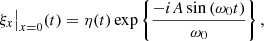
In order to be able to make progress in the analytical derivations, the model uses a Cartesian coordinate system (x, y, z), where x = 0 is the interface and the z-direction is the longitudinal direction (i.e., along the cylinder’s axis). The region x < 0 represents the interior of the structure, whereas the region x > 0 represents the surrounding plasma. This is a model for the local stability at the boundary, in the region of the structure where the shear in longitudinal velocity is the greatest, that is to say, at an antinode of the longitudinal component of the velocity eigenfunction. For the longitudinally fundamental slow mode, this would be at the middle of the structure (see Fig. 1), whereas for the first longitudinal overtone, for example, this would be at a quarter of the structure’s length measured from either end. The time variable is denoted by t.
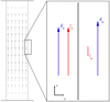 |
Fig. 1. Sketch of a longitudinal cut along the axis of a coronal loop harboring a fundamental standing slow body sausage mode, at the velocity’s maximal amplitude (left) and the local cartesian model at the boundary (right). The arrows on the left represent the velocity field and their lengths are to scale with the relative local magnitude of the field for a slow body sausage mode at a given time. The lengths and directions of the magnetic field arrows on the right figure are consistent for that same slow mode, whereas for the velocity arrows only the direction is consistent (the length of the exterior velocity arrow having been increased for visual clarification). |
After linearizing the ideal MHD equations, the equilibrium quantities are denoted by the subscript 0 and the perturbed quantities are denoted by the subscript 1. The regions on each side of the interface are two homogeneous but different plasmas. This means each region has its own values for the background quantities, which are assumed spatially constant. The background magnetic field is assumed to be a straight and constant axial field along the z-coordinate: B0 = B0z1z. Furthermore, we assume that the background flow is oscillating with a certain frequency ω0, which represents the frequency of the standing slow wave: v0 = V0cos(ω0t)1z. It would, of course, be more accurate to also include a background oscillation for the other quantities, such as magnetic field, pressure, and density. In the context of solar atmospheric structures, the magnetic field oscillations that occur because of this external forcing in the background can, however, be neglected in a first approximation with respect to the strong longitudinal magnetic field. As for the density and pressure background oscillations, they can be neglected in this model because they are in antiphase with respect to the velocity in their longitudinal profile and thus have a node where the logitudinal component of velocity has an antinode. For slow modes, the longitudinal component of the velocity is typically much larger than its other components (see left of Fig. 1), which can thus be neglected at the former’s antinode as well.
The perturbed density, thermal pressure, velocity and magnetic field are denoted with ρ1, p1, v1 and B1, respectively. In what follows the perturbed eulerian total pressure will be used as well, which is given by  . Although gravity certainly has a role in solar atmospheric wave dynamics, it is neglected in this model in order to make some analytical progress.
The linearized compressible ideal MHD equations can, under these assumptions, be written as follows:


where  is the Lagrangian derivative of a quantity f,
  is the speed of sound and μ0 the magnetic permeability of free space. The first equation, Eq. (1), has this simpler form because ∇ρ0 = 0 in each region (i.e., both inside and outside the cylinder). Since the background quantities depend only on x and t, the perturbed quantities can be Fourier-analyzed in the y and z coordinates and are thus assumed to have the following form:
  , for each of the perturbed quantities p1, ρ1, v1x, v1y, v1z, B1x, B1y and B1z.
3. Expressions for the perturbed quantities
In this section, we derive the governing equations for the evolution of linear MHD perturbations in a compressible plasma for the model described in the previous section. In the next section, we then try to use the obtained information to describe the stability of the interface in compressible plasma conditions.
3.1. The central quantity ∇ ⋅ ξ
In what follows, an expression is derived for the compression term ∇ ⋅ ξ. This term is central to finding expressions for all other physical quantities, in the sense that they can all be derived solely from it.
By using the Lagrangian displacement ξ defined by  , it can be shown (see Appendix A) that the compression term ∇ ⋅ ξ must satisfy the following partial differential equation:
where  and
and  is the Alfvén speed. This partial differential equation is of fourth order in t and second order in x. Note that if V0 = 0, such that the time dependence of the background quantities disappears, we retrieve an ordinary differential equation (ODE) of second order in x which is the governing equation for the compression term ∇ ⋅ ξ in a plasma without a background flow. This is the equation used for example in Edwin & Roberts (1983) to study wave modes in a magnetic cylinder in the framework of ideal MHD in a plasma without background flow.
By drawing inspiration from the derivations of Barbulescu et al. (2019), one finds that Eq. (5) can take a simpler form if ∇ ⋅ ξ is written as

where  . Since g(t) has modulus equal to 1 for all t ∈ ℝ, the stability of ∇ ⋅ ξ over time is entirely determined by f. Inserting expression (6) into Eq. (5) simplifies this equation considerably, now taking the following form:
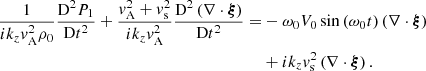
![$$ \begin{aligned} {\frac{\partial ^{4} f(x,t)}{\partial {t}^{4}}}&- \left( {{ v}_{\rm A}}^{2}+{{ v}_{\rm s}}^{2} \right) {\frac{\partial ^{4} f(x,t)}{ \partial {x}^{2}\partial {t}^{2}}}\nonumber \\&+ \left[ i \omega _{0} k_{z} V_{0} \sin \left( \omega _{0} t \right) + k^2 \left( {{ v}_{\rm A}}^{2}+{{ v}_{\rm s}}^{2} \right) \right] {\frac{\partial ^{2} f(x,t)}{\partial {t}^{2}}} \nonumber \\&- \left[ i \omega _{0} k_{z} V_{0} {{ v}_{\rm A}}^{2} \sin \left( \omega _{0} t \right)+{k_{z}}^{2}{{ v}_{\rm A}}^{2}{{ v}_{\rm s}}^{2} \right] {\frac{\partial ^{2} f(x,t)}{\partial {x}^{2}}}\nonumber \\&+ 2 i \omega _{0}^2 k_{z} V_{0} \cos \left( \omega _{0} t \right) {\frac{\partial f(x,t)}{\partial t}}\nonumber \\&+ \left[ i \omega _0 k_z V_0 \sin \left( \omega _0 t \right) \left( k^2 { v}_{\rm A}^2 - \omega _0^2 \right) \right.\nonumber \\&\left. \qquad \qquad \qquad \qquad + k^2 {k_{z}}^{2}{{ v}_{\rm A}}^{2}{{ v}_{\rm s}}^2 \right] f(x,t) = 0 . \end{aligned} $$](/articles/aa/full_html/2021/06/aa40534-21/aa40534-21-eq15.gif)
Equation (7) has a solution in the form of F(x)G(t), where F and G satisfy the following ODEs (with m a constant):
and
with τ = ω0t, and where
![$$ \begin{aligned}&a_1 = \frac{\left({ v}_{\rm A}^2 + { v}_{\rm s}^2 \right) \left(m^2 + k^2 \right)}{\omega _0^2}, \quad q_1 = \frac{i k_z V_0}{\omega _0},\\&q_3 = \displaystyle \frac{2 i k_z V_0}{\omega _0},\\&a_2 = \frac{k_z^2 { v}_{\rm A}^2 { v}_{\rm s}^2 \left( m^2 + k^2 \right)}{\omega _0^4} , \qquad q_2 = \frac{i k_z V_0 \left[ \left( m^2 + k^2 \right) { v}_{\rm A}^2 - \omega _0^2 \right] }{\omega _0^3}\cdot \end{aligned} $$](/articles/aa/full_html/2021/06/aa40534-21/aa40534-21-eq18.gif)
These two equations are related by the constant m, which occurs in both of them.
3.1.1. The spatial function F
Equation (8) has a simple analytical solution, namely

with C1 and C2 arbitrary constants. From this it can be inferred that m plays the role of the wavenumber along x, which is the direction normal to the interface. The focus of this paper goes to standing slow waves in solar atmospheric structures that can be modeled as a straight cylinder with a circular base and a discontinuous boundary separating two homogeneous but different plasma regions. Therefore, each region has its own value for m (namely mi for the interior and me for the exterior), each being able to only take on specific values depending on the boundary conditions at the interface. Finding expressions for mi and me is, however, not straightforward. This will be discussed in Sect. 3.1.2. We note that for the purpose of studying the local stability of the interface, m will be taken purely imaginary in order to have evanescent spatial profiles in the normal direction.
3.1.2. The temporal function G
Equation (9) does not have a simple analytical solution. This equation governs the stability of the compression term ∇ ⋅ ξ over time, its parameters depending on the background quantities vA, vs, V0 and ω0. The function h(t) = G(t)g(t), where G is the solution to Eq. (9), actually describes the general time evolution of ∇ ⋅ ξ in a compressible homogeneous plasma of inifinite extent with an oscillating background velocity which is parallel to the straight and constant equilibrium magnetic field. Although there is no closed-form analytical solution, the boundedness of ∇ ⋅ ξ over time can be derived from the properties of Eq. (9). Indeed, this linear fourth-order ODE has periodic coefficients with the same period and hence it falls in the category of equations which obey Floquet theory (Chicone 2008).
Defining τ = ω0t, it can be rewritten as a 4 × 4 system of first-order ODEs of the form x′(τ) = A(τ)x(τ), where the coefficient matrix A(τ) is periodic with a period of 2π. One can find four linearly independent fundamental solution vectors x1(τ), x2(τ), x3(τ) and x4(τ), which depend on their respective initial conditions. The matrix obtained by putting these four vectors into its columns is called a fundamental solution matrix. If we take as initial condition matrix the identity matrix, Floquet theory states that the corresponding fundamental solution matrix (which we denote by X(τ)) evaluated at one period (i.e., at τ = 2π in our case) is intimately linked to the boundedness of the solutions of the ODE. Indeed, denoting the eigenvalues of X(2π) by λ1, λ2, λ3 and λ4, Floquet’s theorem states that for each distinct eigenvalue λ, if we write λ = e2πμ where μ ∈ ℂ is called the Floquet exponent, there exists an independent solution of the system which has the form
where Φ contains 2π-periodic functions. This means that a solution to Eq. (9) is unstable if and only if |λ| > 1 for at least one eigenvalue λ of X(2π). If there are less than four distinct eigenvalues of X(2π), it is possible there are less than four independent Floquet solutions of the form (11). If the eigenspace of X(2π) has dimension 4, there are still four independent eigenvectors Φi and thus four independent Floquet solutions. If the eigenspace of X(2π) has dimension less than 4, then there are less than four independent Floquet solutions. In that case, extra independent solutions have to be found by using the Jordan normal form of X(2π) (see e.g., Cesari 1963 for more details). These extra independent Jordan solutions are always unstable. The stability of ∇ ⋅ ξ is thus entirely determined by the Floquet exponents μ.
A solution to Eq. (9) can be written in the form of a series. Knowing that each independent Floquet solution has the form eμτΦ(τ) with Φ a 2π-periodic function, one can assume that such a basic independent solution can be written as
where the φj are unknown coefficients. Writing μ = iν for convenience, the following recurence relation between the coefficients φj can then be derived by inserting expression (12) into Eq. (9):

where
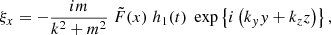
![$$ \begin{aligned} \varepsilon _j = \displaystyle \frac{\frac{1}{2} k_z V_0 \omega _0 \left[ \left( j + \nu \right)^2 \omega _0^2 - K^2 { v}_{\rm A}^2 \right]}{\left( j + \nu \right)^4 \omega _0^4 - \left( j + \nu \right)^2 \omega _0^2 K^2 \left( { v}_{\rm A}^2 + { v}_{\rm s}^2 \right) + k_z^2 K^2 { v}_{\rm A}^2 { v}_{\rm s}^2} \end{aligned} $$](/articles/aa/full_html/2021/06/aa40534-21/aa40534-21-eq23.gif)
with  . Equation (13) are nontrivially satisfied if and only if the following infinite determinant vanishes:
This is a Fredholm determinant. Denoting with A the operator defined by the corresponding infinite matrix, this Fredholm determinant is well-defined if the operator A − I (where I is the identity operator) is a trace class operator on ℓ2(ℤ), the Hilbert space of square-summable sequences of complex numbers with entire index. It can be shown that this is the case here (see for example Sträng 2005 for the method to follow), except if the denominator of one of the εj vanishes. This happens if the perturbation, which is a normal mode with wave vector K = (m, ky, kz), satisfies the equation
![$$ \begin{aligned} (j+\nu )^2 \omega _0^2 = \displaystyle \frac{K^2 \left({ v}_{\rm A}^2 + { v}_{\rm s}^2 \right)}{2} \left\{ 1 \pm \left[ 1 - \displaystyle \frac{4 k_z^2 { v}_{\rm A}^2 { v}_{\rm s}^2}{K^2 \left( { v}_{\rm A}^2 + { v}_{\rm s}^2 \right)^2} \right]^{1/2} \right\} , \end{aligned} $$](/articles/aa/full_html/2021/06/aa40534-21/aa40534-21-eq26.gif)
for a j ∈ ℤ. This represents a resonance between the background oscillator with frequency ω0 and a magnetosonic wave, in a homogeneous plasma of infinite extent. In this case m is a free parameter (like ky and kz) and can potentially take any real value. In the model we describe in this paper, with an interface separating two such homogeneous plasmas, only certain specific values of m (different in both regions) are physically possible. Because surface waves on the interface are actually of interest in this case, m should be imaginary. In Sect. 4 we study the resonance of these surface waves with the background oscillator.
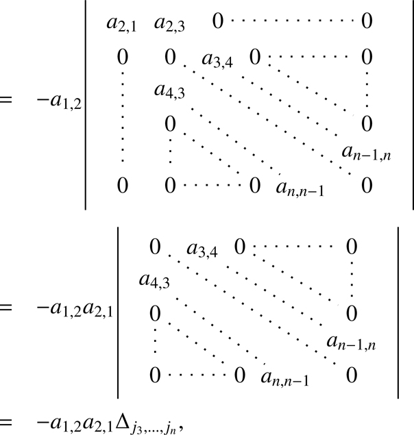
Considering Δ as a function of the two unknowns ν and m, it is thus well-defined for every (ν, m) except in the poles of the εj. It can also easily be checked with Eqs. (14) and (15) that Δ(ν, m) = Δ(ν + 1, m) and Δ(ν, m) = Δ(−ν, m). As previously stated, there are in general four independent Floquet solutions of the form (12) to Eq. (9). Hence, all solutions for ν of Δ(ν, m) = 0 (as functions of m) which correspond to distinct solutions of the differential equation lie on the strip −0.5 < Re[ν] ≤ 0.5. These distinct solutions relate as follows: ν2 = −ν1 and ν4 = −ν3. The four independent Floquet solutions in the most general case are thus of the form eμ1τΦ1(τ), e−μ1τΦ2(τ), eμ3τΦ3(τ) and e−μ3τΦ4(τ), where Φ1, Φ2, Φ3 and Φ4 are 2π-periodic functions. Recalling the earlier discussion in this section, we note that it is possible that there are less than four independent Floquet solutions if at least two eigenvalues λj = e2πiνj of X(2π) are equal. From the properties of Δ, we can see that this happens in two situations. One possibility is if we have Re[νj] = n/2 for some n ∈ ℤ and Im[νj] = 0, for one of the solutions νj. Indeed, the eigenvalues e2πiνj and e−2πiνj are equal in that case. Another possibility is if, for two solutions νj and νl, we have Re[νj] = Re[νl]+n for some n ∈ ℤ and Im[νj] = Im[νl]. In this case e2πiνj and e2πiνl will also be equal.
We find the following formula for Δ, derived in Appendix B:
![$$ \begin{aligned} \Delta = 1 + \displaystyle \sum _{n=1}^{\infty } \left[ \displaystyle \sum _{j_1 = - \infty }^{\infty } \displaystyle \sum _{j_2 = j_1 + 2}^{\infty } \ldots \displaystyle \sum _{j_n = j_{n-1} + 2}^{\infty } \left( \displaystyle \prod _{l=1}^n \varepsilon _{j_l} \varepsilon _{j_l +1} \right) \right]. \end{aligned} $$](/articles/aa/full_html/2021/06/aa40534-21/aa40534-21-eq27.gif)
It is clear from Eq. (14) that  as |j| → ∞. We can then try to use the fact that εj drops off as 1/j2 to approximate the cumbersome formula (17). If we can assume that |Im[ν]| ≪ |Re[ν]|, then since −0.5 < Re[ν] ≤ 0.5 the quantity ν becomes negligible with respect to j already for quite small |j| in that case. In Sect. 4, we see that this is a good assumption in both coronal and photospheric conditions, if the Alfvén Mach number MA = (V0i − V0e)/vAi is small enough.
One could then try considering, as a first approximation for Δ, only the first few terms on the right-hand side of Eq. (17). Taking n = 1 and j1 ∈ { − 1, 0, 1}, this would yield:

Equation (18) corresponds to Eq. (15) with the infinite determinant in the right-hand side truncated to a 3 × 3 determinant centered on the row with ε0. If one starts from the incompressible versions of Eqs. (1)–(4), one can derive that m = ik in an incompressible plasma. The approximation of truncating the series in Eq. (17) is only valid for large enough |j| and away from the poles of the εj. Under the assumption that |K|vA ≪ ω0 and |K|vs ≪ ω0, this condition is fulfilled. We note that in the solar atmosphere, vA and vs are rougly of the same order of magnitude. Since K = k2 − |m|2 for surface waves, we have K → 0 in the incompressible limit. Equation (18) thus gives us an approximation for Δ at least in a weakly compressible plasma, but could maybe even be correct more generally.
Analytical solutions for mi and me in function of ν can then be derived from Eq. (18). The obtained expressions for mi(ν) and me(ν) are very complicated but, introducing numerical values relevant for the physical conditions of the solar structure being considered, we can use them together with a third relation involving ν, mi and me. This other relation can theoretically be the one derived in the next subsection, although in practice one of those we derive in Sect. 4 under approximating circumstances will probably be preferred. We note that ν is the same on both sides of the interface, as will be explained in the next section. In contrast to this, m is in general not identical on both sides. It can also be seen that Δ(ν, m) = Δ(ν, −m). Hence, if m is a solution then so is −m. This is reflected in the form of the spatial function F in Eq. (10).
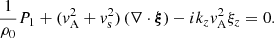
3.2. Other perturbed physical quantities
With h(t) = G(t)g(t), the compression term can be written as ∇ ⋅ ξ = F(x)h(t)exp{i(kyy + kzz)}. From this and Eqs. (1)–(4), the following expressions for the perturbed quantities can then easily be derived:


with  and where h1, h2, h3 are still unknown but have to satisfy
by the definition ∇ ⋅ ξ = ∂ξx/∂x + ∂ξy/∂y + ∂ξz/∂z. Each of the expressions (19)–(27) is different for each region on both sides of the interface. The functions  , F, h, h1, h2 and h3 in particular will have a different version in both regions. For the spatial functions
  and F, only one of the two coefficients C1 and C2 must be retained in each region. We make the choice that C1 = 0 in the x < 0 region, and C2 = 0 in the x > 0 region.
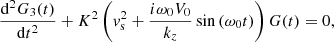
Writing h1(t) = G1(t)g(t), h2(t) = G2(t)g(t) and h3(t) = G3(t)g(t), the following expressions for G1, G2 and G3 can be derived from Eqs. (1)–(3), (19)–(21) and (27) (see Appendix C):
It can also be checked that Eq. (28) is indeed fulfilled with these expressions. Now, the following two boundary conditions have to be fulfilled at the interface between the two regions (i.e., at x = 0) for physical reasons:
![$$ \begin{aligned}&[\xi _x] = 0, \end{aligned} $$](/articles/aa/full_html/2021/06/aa40534-21/aa40534-21-eq45.gif)
![$$ \begin{aligned}&[P_1] = 0, \end{aligned} $$](/articles/aa/full_html/2021/06/aa40534-21/aa40534-21-eq46.gif)
where [f] = limx ↓ 0f(x)−limx ↑ 0f(x) denotes the jump in a quantity f across the interface. We note that, similarly as for the frequency of a normal mode in the case without background flow, ν is the same inside and outside. It has proven to be too difficult to show mathematically, but it can be explained as follows. When a perturbation is unstable, its growth rate is determined solely by ν: the growth of every perturbed quantity is namely expressed by the factor e−Im[ν]t. Therefore, since quantities such as ξx and P1 have to be continuous at the interface x = 0, ν must be the same on both sides of the interface.
From the two Eqs. (31) and (32) linking the interior and exterior solutions, a relation can be derived which has to be satisfied in order for the system determined by these equations to have nontrivial solutions:
where
![$$ \begin{aligned}&\zeta _{A,j} = \displaystyle \sum _{l=- \infty }^{\infty } \frac{2 \omega _0^2 { v}_{\rm si}^2 { v}_{\rm se}^2 \left[ \left( l+\nu \right)^2 \omega _0^2 - k_z^2 { v}_{\rm Ai}^2 \right] \varphi _{l,\mathrm{i}} \varphi _{j-l,\mathrm{e}}}{\left[ \left( l+\nu \right)^2 \omega _0^2 - K_{\rm i}^2 { v}_{\rm Ai}^2 \right] \left[ \left(j- l+\nu \right)^2 \omega _0^2 - K_{\rm e}^2 { v}_{\rm Ae}^2 \right]} , \\&\zeta _{B,j} = \displaystyle \sum _{l=- \infty }^{\infty } \frac{2 \omega _0^2 { v}_{\rm si}^2 { v}_{\rm se}^2 \left[ \left( l+\nu \right)^2 \omega _0^2 - k_z^2 { v}_{\rm Ae}^2 \right] \varphi _{l,\mathrm{e}} \varphi _{j-l,\mathrm{i}}}{\left[ \left( l+\nu \right)^2 \omega _0^2 - K_{\rm e}^2 { v}_{\rm Ae}^2 \right] \left[ \left(j- l+\nu \right)^2 \omega _0^2 - K_{\rm i}^2 { v}_{\rm Ai}^2 \right]} . \end{aligned} $$](/articles/aa/full_html/2021/06/aa40534-21/aa40534-21-eq48.gif)
Equation (33), arising from the boundary conditions at the interface, is usually called the dispersion relation when there is no oscillating background flow. Both mi and me being determined by Eq. (15) (by inserting respectively interior and exterior values for the background quantities), Eq. (33) determines the only remaining unknown, ν.
From Eq. (33), the following has to hold for every j ∈ ℤ:
For j = 0 this gives us the relation
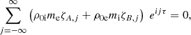
![$$ \begin{aligned} \displaystyle \frac{m_{\rm e}}{m_{\rm i}} = - \displaystyle \frac{\rho _{\rm 0e}}{\rho _{\rm 0i}} \displaystyle \frac{\displaystyle \sum _{l=- \infty }^{\infty } \frac{ \left[ \left( l+\nu \right)^2 \omega _0^2 - k_z^2 { v}_{\rm Ae}^2 \right] \varphi _{l,\mathrm{e}} \varphi _{-l,\mathrm{i}}}{\left[ \left( l+\nu \right)^2 \omega _0^2 - K_{\rm e}^2 { v}_{\rm Ae}^2 \right] \left[ \left(l-\nu \right)^2 \omega _0^2 - K_{\rm i}^2 { v}_{\rm Ai}^2 \right] } }{ \displaystyle \sum _{l=- \infty }^{\infty } \frac{\left[ \left(l -\nu \right)^2 \omega _0^2 - k_z^2 { v}_{\rm Ai}^2 \right] \varphi _{l,\mathrm{e}} \varphi _{-l,\mathrm{i}}}{\left[ \left( l+\nu \right)^2 \omega _0^2 - K_{\rm e}^2 { v}_{\rm Ae}^2 \right] \left[ \left(l-\nu \right)^2 \omega _0^2 - K_{\rm i}^2 { v}_{\rm Ai}^2 \right] } }\cdot \end{aligned} $$](/articles/aa/full_html/2021/06/aa40534-21/aa40534-21-eq50.gif)
We note that this is not an explicit solution for me/mi, because both mi and me appear on the right-hand side, through Ki and Ke respectively. While Eq. (35) seems difficult to use directly, it gives us some information. Indeed, we learn from this equation that, whereas in the incompressible case we have me/mi = 1, in the compressible case me/mi seems to depend on kz as well as ky, the latter appearing only in Ki and Ke. In the next section, we see that the only perturbation quantities the stability of the interface depends on are kz and me/mi. This means that, while the abstraction is made that only the longitudinal wavenumber kz is important for the stability of the interface in an incompressible plasma, the perpendicular wavenumber ky seems to have some influence as well in the more realistic case of a compressible plasma.
4. Stability of the interface
4.1. Governing equation
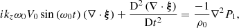
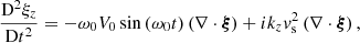
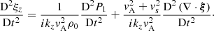
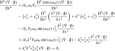
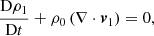
The results derived in the preceding sections permit us to say something about the stability of the interface at the structure’s boundary. This stability is determined by the temporal evolution of the normal displacement ξx, which is governed by the following equation:
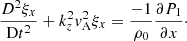
There is again a different version of Eq. (36) for each region, namely for x < 0 and for x > 0. For each of the two regions, the respective versions of expression (27) for P1 can then be inserted in the respective versions of Eq. (36). These can then be put together by expressing C1 in function of C2 thanks to Eq. (32), and yield the following equation governing the displacement of the interface over time:
where Di/Dt = ∂/∂t + ikzV0isin(ω0t), De/Dt = ∂/∂t + ikzV0esin(ω0t), and ξx|x = 0 is ξx evaluated at x = 0.
Using a similar trick as was used for ∇ ⋅ ξ before and which was also used by Barbulescu et al. (2019) in a different setup, we write ξx|x = 0 as
with 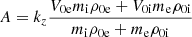 . This assumption changes nothing to the stability of ξx|x = 0(t) since the moduli of ξx|x = 0(t) and η(t) are the same for every t ∈ ℝ+, and therefore ξx|x = 0 is unbounded if and only if η is unbounded. Inserting Eq. (38) in Eq. (37) greatly simplifies the equation, which can be worked out to yield the following ODE for η:
with τ = ω0t and
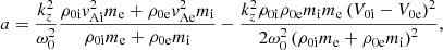
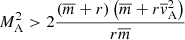
The parameters a and q can be rewritten in normalized form as follows:
![$$ \begin{aligned}&a = \kappa _z^2 \left[ \displaystyle \frac{\overline{m} + r \overline{{ v}}_{\rm A}^2}{\overline{m} + r} - \frac{r \overline{m} M_{\rm A}^2}{2 \left( \overline{m} + r \right)^2} \right] , \end{aligned} $$](/articles/aa/full_html/2021/06/aa40534-21/aa40534-21-eq58.gif)
where we introduced the normalized quantities κz = kzvAi/ω0,  , r = ρ0e/ρ0i,
  and MA = (V0i − V0e)/vAi.
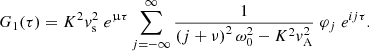
We notice that the first term of a consists of an expression that resembles the squared kink frequency and which we call the pseudo squared kink expression. The second term of a resembles a Doppler-shifting correction and equals −2q. In an incompressible plasma, the first term would be the squared kink frequency (since then mi, me → k). We also note that if there is no background flow (i.e., V0i = V0e = 0), we are left with only the pseudo squared kink expression in the factor in front of η(τ) in Eq. (39). The solution is then a surface wave with frequency ν determined by the dispersion relation
where mi and me are determined in function of ν through their respective version of Eq. (17). Equation (44) is a transcendental equation in ν with more than one solution, which means that there are several different modes in a compressible plasma. This is in contrast with an incompressible plasma, where there is only one mode, for which the expression of the frequency is readily readable from Eq. (44) and is equal to the kink frequency. These results about modes at an interface in a compressible plasma without background flow are already known (see for example Priest 2014).
4.2. Instability conditions
Equation (39) is the Mathieu equation, which also pertains to the class of equations obeying Floquet theory and which has been extensively studied for example by McLachlan (1947). It does not have an analytical solution but the stability of its solution in function of its parameters is well-known. The stability of the solutions of the Mathieu equation (39) in function of the parameters a and q is often represented in the so-called stability diagram (see Fig. 2). The white zones in the figure are regions where the solutions are stable, whereas the gray zones are region where the solutions are unstable.
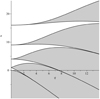 |
Fig. 2. Stability diagram of the Mathieu equation. The white zones represent regions of the parameter space where the solution is stable, whereas the gray zones represent regions of the parameter space where the solution is unstable. |
4.2.1. Constant shear flow
In order to gain some insight on the nature of the potential instabilities, we follow Hillier et al. (2019), who studied the stability of an interface in a similar model. We start by looking at the case with a constant background shear flow (i.e., we assume ω0 = 0). We have to modify the procedure above a little bit in order to be mathematically correct: instead of Eq. (38), we assume ξx|x = 0(t) = η(t)exp{−iAt} in this particular case. The obtained equation is then
![$$ \begin{aligned} \displaystyle \frac{\mathrm{d}^2 \eta (\tau )}{\mathrm{d} \tau ^2} + \kappa _z^2 \left[ \displaystyle \frac{\overline{m} + r \overline{{ v}}_{\rm A}^2}{\overline{m} + r} - \frac{r \overline{m} M_{\rm A}^2}{\left( \overline{m} + r \right)^2} \right]\; \eta (\tau ) = 0. \end{aligned} $$](/articles/aa/full_html/2021/06/aa40534-21/aa40534-21-eq63.gif)
It has normal mode solutions with normalized frequency ν defined by the dispersion relation
![$$ \begin{aligned} \nu ^2 = \kappa _z^2 \left[ \displaystyle \frac{\overline{m} + r \overline{{ v}}_{\rm A}^2}{\overline{m} + r} - \frac{r \overline{m} M_{\rm A}^2}{\left( \overline{m} + r \right)^2} \right]\cdot \end{aligned} $$](/articles/aa/full_html/2021/06/aa40534-21/aa40534-21-eq64.gif)
This transcendental equation in ν has multiple solutions as well, and thus we see that there are also different modes in the case of a constant shear flow in a compressible plasma. A particular mode will be unstable to the KHI if
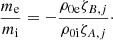
is satisfied. Different modes will thus have different instability conditions in a compressible plasma. If we take the incompressible limit, the above derivations match the already well-known results of a constant shear flow in an incompressible plasma (see for example Chandrasekhar 1961).
4.2.2. Oscillating shear flow
In the case of an oscillatory background flow (ω0 ≠ 0), Eq. (39) governs the evolution of the normal displacement at the interface over time. In the same way as for Eq. (9), Floquet theory allows us to write an independent solution to the Mathieu equation as follows (McLachlan 1947):
This resembles a normal mode with frequency ν, but with a periodic function replacing the constant. One can then find the following recursion relation by inserting Eq. (48) into Eq. (39):

where
If the denominator of one of the ϵj vanishes, there can be a resonance between the background oscillator and the induced surface waves.
Now some analytical progress can be made in the limiting case q → 0, corresponding to a small squared shear rate  with respect to the squared frequency
  . Indeed, for q ≪ 1, we see from Eq. (49) that in order to have a nontrivial solution (48) we need the denominator of at least one of the ϵj to vanish. For that, we need to have
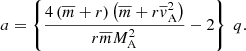
for a j ∈ ℤ. In case ν2 ≈ a, that is to say, if
![$$ \begin{aligned} \nu ^2 \approx \kappa _z^2 \left[ \displaystyle \frac{\overline{m} + r \overline{{ v}}_{\rm A}^2}{\overline{m} + r} - \frac{r \overline{m} M_{\rm A}^2}{2 \left( \overline{m} + r \right)^2} \right], \end{aligned} $$](/articles/aa/full_html/2021/06/aa40534-21/aa40534-21-eq72.gif)
then Eq. (16) is fulfilled for j = 0. Since Eq. (52) is again a transcendental equation in ν with multiple solutions, there are multiple modes possible. These modes are surface waves with frequency ν. Such a mode will be unstable if
is satisfied. This renders the right-hand side in Eq. (52), which is a, negative. Hence, for q ≪ 1, the region of the parameters space which corresponds to the KHI is a < 0. It can be seen on Fig. 2 that this region is indeed uniformly unstable. We note that the right-hand side in Eq. (53) is a factor of 2 larger than in Eq. (47). In a first approximation, we could thus evaluate the minimum value of MA for the KHI to develop in the case of an oscillatory shear flow with q ≪ 1 to be  times higher than in the case of a constant shear flow with q ≪ 1. This is assuming that the corresponding values of mi and me are equal in both cases. In an incompressible plasma, this is obviously correct. In a compressible plasma, however, there is no reason to suggest a priori that this is the case in general. Nevertheless, the values might still be close, such as in a weakly compressible plasma for example.
If on top of Eq. (51) being satistfied for j = 0 it is also satisfied for another j ∈ ℤ, then there is a resonance between a mode satisfying Eq. (52) and the background oscillator. From ν2 = a and Eq. (16) with j ≠ 0, this means that we must have

In Fig. 2 we see the regions of resonance instability around a = j2, with j ∈ ℤ0. Hence, for q ≪ 1, the KHI and the resonance instability are clearly distinct features and are mutually exclusive.
As was also mentionned by Hillier et al. (2019) (themselves based on Bender & Orszag 1999), the dominant resonance in this limit is the one with j = 1. Its instability reagion is borded by the curves

and its maximum growth rate is
![$$ \begin{aligned} \mathrm{Im}[\nu ] = \displaystyle \frac{q}{2} + O(q^2) \qquad \mathrm{as}\,q \rightarrow 0. \end{aligned} $$](/articles/aa/full_html/2021/06/aa40534-21/aa40534-21-eq77.gif)
We could thus express this growth rate through the equation ![$ \mathrm{Im}[\nu] = \frac{q}{2} $](/articles/aa/full_html/2021/06/aa40534-21/aa40534-21-eq78.gif) as an approximation. This is an implicit equation in ν, because q depends on it through
as an approximation. This is an implicit equation in ν, because q depends on it through  .
.
4.3. Solar applications: Relevant region of the parameter space
From Eqs. (42) and (43), we see the parameters a and q are related as follows:
In the incompressible limit,  and we find the same relation as Barbulescu et al. (2019) for their model. For fixed values of the background quantities and for a fixed value of
  , Eq. (57) represents a line in the aq-plane. We note, however, that changing the value of kz and/or ky a priori changes the value of
  as well and that hence the modes do not lie all on the same line. This is unlike the case of an incompressible plasma, where one stays on the same line when changing kz, as was already found for example by Barbulescu et al. (2019) in a similar model.
We find that the slope in Eq. (57) is minimized for  , in which case the line’s equation is
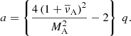
For each set of fixed background quantities, the only physically possible values of a and q thus lie in the region of the stability diagram between the positive a-axis and the line defined by Eq. (58). We see that, in this model, it is not physically possible to have values of (q, a) in the region below the line through the origin and with slope −2.
4.3.1. Coronal loops
A first application to a solar atmospheric structure would be a coronal loop, where slow waves occur near footpoints (De Moortel et al. 2002) or during flares (Wang et al. 2002; Kumar et al. 2013). For a standing slow wave under realistic coronal loop conditions, for which we took (vAe, vsi, vse) = (5/2, 1/2, 1/4)vAi, the line of minimum slope, Eq. (58), lies almost on the positive a-axis. Indeed, with  and for MA = 0.066 for example, we find the line of minimum slope to be given by a = 11415q. If we assume incompressibility and fix
  , Eq. (57) defines a line as well and we find a = 12486q. For the less realistic value of MA = 1, we find that the line of minimum slope is given by a = 47q whereas in the incompressible limit the line (57) becomes a = 52q. This is summarized in Table 1. As we can see from Fig. 2, the region of the aq-diagram relevant for coronal loop conditions is thus stable with respect to the KHI. It could be unstable with respect to resonance; however, since in reality a finite cylindrical structure is closed both azimuthally and longitudinally, the respective wavenumbers will take on discrete values. In the aq-diagram, the possible values will thus be a set of discrete points (an, qn). Seeing how the vast majority of the area is a stable region in the relevant region between the positive a-axis and the minimum-slope line (58), it is likely that this parametric resonance instability is avoided as well.
We conclude that the oscillating shear velocity of a standing slow wave in a coronal loop would not trigger the KHI on its own, without the involvement of other physical processes. This is in clear contrast with the fast kink waves. Indeed, according to the incompressible models of Barbulescu et al. (2019) and Hillier et al. (2019), which are similar to this model but where the velocity and magnetic fields are perpendicular instead of parallel, fast kink waves are predicted to excite the KHI on the loop boundary. This has also been confirmed by numerical simulations.
4.3.2. Photospheric pores
As was mentioned in the introduction, propagating slow waves have also been observed in photospheric pores. One would be curious whether standing versions of these modes could trigger the KHI under these conditions. The model can be used to examine the stability of slow waves in these structures as well. However, the qualitative conclusion is the same as in the case of coronal loops: with photospheric pore conditions set to (vAe, vsi, vse) = (1/4, 1/2, 3/4)vAi, we have  , and, taking MA = 0.066, the minimum slope is 1450 whereas for the slope of the line defined by Eq. (57) is 1615 in the incompressible limit. As a comparison, even for the unrealistic value of MA = 1, the minimum slope is 4.25 and the slope in Eq. (57) in the incompressible limit is 5. This is again summarized in Table 1. These values are an order of magnitude lower then for their coronal counterpart, but looking at Fig. 2 we see that the same conclusion remains: every possible pair of parameters (a, q) lie in a region that does not permit the development of the KHI. Similarly as for a coronal loop in the previous subsection, it is likely that the parametric instability arising from resonance with the driver is also avoided and that the pore therefore remains stable.
Additionally, one could investigate the stability of resonant slow waves, which can occur in the presence of a transition layer at the pore’s boundary. Indeed, slow surface waves are known to be resonantly absorbed in photospheric conditions. It is worth wondering whether the great longitudinal velocity shear that arises around the resonant point could be enough to trigger the KHI. In ideal MHD, the longitudinal velocity of resonant slow modes displays a hyperbolic singularity (Sakurai et al. 1991), but in the presence of finite resistivity this singularity disappears to make place for a sharp but continuous profile. Kovitya & Cram (1983) reported values of electrical resistivity in sunspots, with a minimum resistivity corresponding to a magnetic Reynolds number of 107. Erdelyi (1997) derived an expression for the longitudinal Lagrangian displacement in the dissipative layer around the cusp resonance in the presence of finite electrical resistivity (see Eq. (30) therein). Assuming a sinusoidal transition profile with width l = 0.1R (where R is the radius of the pore) in the squared cusp and sound speeds, a ratio of external to internal magnetic field of B0ze/B0zi = 0.33, a cusp resonant position at rC = 0.955R (based on the numerical computations of Goossens et al. 2021), a value for the perturbed total pressure at the resonant position equal to its value on the interface for the corresponding surface mode in the absence of the transition layer, a real part of the frequency equal to the frequency of the corresponding surface mode in the absence of the transition layer, and a magnetic Reynolds number of 107 to have a lowerbound on resistivity and thus an upperbound on realistic values for the longitudinal velocity at the resonance, we found a value of MA = 0.36 around the cusp resonance point for a sausage mode with kzR = 2. This value of kzR is within the range of validity for the longitudinal wavenumber of the observed slow surface sausage mode in a photospheric pore by Grant et al. (2015). The value found for MA implies a minimum slope of 46 in Eq. (58) and a slope of 52 for Eq. (57) in the incompressible limit. These values are still well above the values for the slopes found for MA = 1 in photospheric conditions. Through the model derived in this paper, we conclude from this that even resonant slow waves do not display a large enough velocity shear for an instability to develop.
4.4. Limitations of the model
We point out that the local model discussed in this paper is only valid under certain conditions. Firstly, the azimuthal wavenumber of the perturbation must be large, such that the azimuthal direction can be approximated by the cartesian direction of y. This means that we must have kyR ≫ 1, with R the structure’s radius. Secondly, for the amplitude of the oscillating background velocity to be assumed constant, the longitudinal wavelength of the perturbation must be small with respect to the structure’s length L. We must thus have kzL ≫ 1. Lastly, we note that our model might not be suitable in the presence of a smooth transition layer between the interior and the exterior of the structure. Indeed, resonant absorption of the standing slow wave in the background could occur in that case (Yu et al. 2017), which leads to a steep and continuous variation in the longitudinal component of the velocity along the x direction. Although one can use the model to estimate the effect of the logitudinal velocity shear in resonant absorption on the stability of the interface, as we did in last subsection, one must keep in mind that certain assumptions on which the model is based are not fulfilled in the presence of a transition layer. Firstly, there is no true discontinuous interface and, secondly, the assumption of a constant amplitude profile along x for the oscillating background velocity is violated.
5. Conclusion
In this paper, we developed an analytical model for the local stability of a cylindrical solar atmospheric structure harboring a standing slow wave. We assumed that the structure is a straight cylinder with a circular base, of which the boundary is an interface discontinuously separating two homogeneous and compressible plasmas. The magnetic fields on both sides were assumed to be constant, straight and aligned with the interface. The velocity fields were assumed to be oscillating in time but spatially constant, in order to model the standing slow wave in the background.
We used linearized MHD to derive an equation for the compression term, ∇ ⋅ ξ. The expressions for all the other perturbed quantities could then be expressed in terms of the solution of ∇ ⋅ ξ. The spatial part of the solution along the direction normal to the interface could be analytically found to be a normal mode, with wavenumber m. In contrast to the incompressible approximation, the value of this wavenumber m in a compressible plasma is different on both sides of the interface. We saw that me/mi is dependent on both kz and ky, which entails that the stability of the interface depends on ky as well as kz. This is in contrast with the incompressible version of this model, in which only kz has an influence on said stability.
We then found that the governing equation for the displacement component of the perturbation normal to the interface is a Mathieu equation. The stability of the solution of this equation in function of the different involved parameters being known from the litterature, we were able to describe two kinds of instabilities that could theoretically arise in the presence of an oscillating shear background flow. As an application to the solar atmosphere, we found that the physically relevant region of the parameter space corresponds to an interface that is locally stable with respect to the KHI, both in a coronal loop and in a photospheric pore. Although the interface can be unstable to a parametric resonance between the background slow wave and the induced perturbations on the interface, we concluded that it is unlikely to happen in reality. Even in the case of resonance in the cusp continuum, we concluded from our model that the longitudinal velocity shear of the resonant slow waves is not enough to trigger an instability.
We ended by noting that this model is only applicable under specific conditions. It is indeed a local model, in the sense that the spatial scale of azimuthal variations must be small compared to the structure’s radius and the spatial scale of longitudinal variations must be small with respect to the loop’s length. Furthermore, for a structure with a smooth transition layer the assumptions of a discontinuous transition at the boundary and a constant amplitude for the background oscillating velocity fields would be violated. This needs to be kept in mind when using this model to infer stability conditions around resonances.
Acknowledgments
M.G. was supported by the C1 Grant TRACEspace of Internal Funds KU Leuven (number C14/19/089). TVD was supported by the European Research Council (ERC) under the European Union’s Horizon 2020 research and innovation programme (grant agreement No 724326) and the C1 grant TRACEspace of Internal Funds KU Leuven.
References
- Afanasyev, A., Karampelas, K., & Van Doorsselaere, T. 2019, ApJ, 876, 100 [Google Scholar]
- Antolin, P., Yokoyama, T., & Van Doorsselaere, T. 2014, ApJ, 787, L22 [NASA ADS] [CrossRef] [Google Scholar]
- Antolin, P., Okamoto, T. J., De Pontieu, B., et al. 2015, ApJ, 809, 72 [NASA ADS] [CrossRef] [Google Scholar]
- Antolin, P., De Moortel, I., Van Doorsselaere, T., & Yokoyama, T. 2017, ApJ, 836, 219 [NASA ADS] [CrossRef] [Google Scholar]
- Arregui, I. 2015, Philos. Trans. R. Soc. London Ser. A, 373, 20140261 [Google Scholar]
- Barbulescu, M., Ruderman, M. S., Van Doorsselaere, T., & Erdélyi, R. 2019, ApJ, 870, 108 [Google Scholar]
- Bender, C., & Orszag, S. 1999, Advanced Mathematical Methods for Scientists and Engineers I: Asymptotic Methods and Perturbation Theory, Advanced Mathematical Methods for Scientists and Engineers (New York: Springer-Verlag) [Google Scholar]
- Berghmans, D., & Clette, F. 1999, Sol. Phys., 186, 207 [NASA ADS] [CrossRef] [Google Scholar]
- Cadez, V. M., Csik, A., Erdelyi, R., & Goossens, M. 1997, A&A, 326, 1241 [NASA ADS] [Google Scholar]
- Cesari, L. 1963, Asymptotic Behavior and Stability Problems in Ordinary Differential Equations (New York: Springer-Verlag) [Google Scholar]
- Chandrasekhar, S. 1961, Hydrodynamic and Hydromagnetic Stability (Oxford: Clarendon Press) [Google Scholar]
- Chen, S.-X., Li, B., Shi, M., & Yu, H. 2018, ApJ, 868, 5 [Google Scholar]
- Chen, S. X., Li, B., Van Doorsselaere, T., Goossens, M., & Geeraerts, M. 2021, ApJ, 908, 230 [Google Scholar]
- Chicone, C. 2008, Ordinary Differential Equations with Applications, Texts in Applied Mathematics (New York: Springer-Verlag) [Google Scholar]
- Conway, J. 1990, A Course in Functional Analysis, Graduate Texts in Mathematics (New York: Springer-Verlag) [Google Scholar]
- De Moortel, I., & Hood, A. W. 2003, A&A, 408, 755 [NASA ADS] [CrossRef] [EDP Sciences] [Google Scholar]
- De Moortel, I., Ireland, J., & Walsh, R. W. 2000, A&A, 355, L23 [NASA ADS] [Google Scholar]
- De Moortel, I., Ireland, J., Walsh, R. W., & Hood, A. W. 2002, Sol. Phys., 209, 61 [NASA ADS] [CrossRef] [Google Scholar]
- De Moortel, I., Pascoe, D. J., Wright, A. N., & Hood, A. W. 2016, Plasma Phys. Control. Fusion, 58, 014001 [Google Scholar]
- Dorotovič, I., Erdélyi, R., & Karlovský, V. 2008, in Waves& Oscillations in the Solar Atmosphere: Heating and Magneto-Seismology, eds. R. Erdélyi, & C. A. Mendoza-Briceno, IAU Symp., 247, 351 [Google Scholar]
- Dorotovič, I., Erdélyi, R., Freij, N., Karlovský, V., & Márquez, I. 2014, A&A, 563, A12 [NASA ADS] [CrossRef] [EDP Sciences] [Google Scholar]
- Edwin, P. M., & Roberts, B. 1983, Sol. Phys., 88, 179 [Google Scholar]
- Erdelyi, R. 1997, Sol. Phys., 171, 49 [Google Scholar]
- Erdélyi, R., Ballai, I., & Goossens, M. 2001, A&A, 368, 662 [EDP Sciences] [Google Scholar]
- Foullon, C., Verwichte, E., Nakariakov, V. M., Nykyri, K., & Farrugia, C. J. 2011, ApJ, 729, L8 [NASA ADS] [CrossRef] [Google Scholar]
- Freij, N., Dorotovič, I., Morton, R. J., et al. 2016, ApJ, 817, 44 [Google Scholar]
- Geeraerts, M., Van Doorsselaere, T., Chen, S.-X., & Li, B. 2020, ApJ, 897, 120 [Google Scholar]
- Goossens, M., Hollweg, J. V., & Sakurai, T. 1992, Sol. Phys., 138, 233 [Google Scholar]
- Goossens, M., Andries, J., & Aschwanden, M. J. 2002, A&A, 394, L39 [NASA ADS] [CrossRef] [EDP Sciences] [Google Scholar]
- Goossens, M., Chen, S. X., Geeraerts, M., Li, B., & Van Doorsselaere, T. 2021, A&A, 646, A86 [EDP Sciences] [Google Scholar]
- Grant, S. D. T., Jess, D. B., Moreels, M. G., et al. 2015, ApJ, 806, 132 [Google Scholar]
- Guo, M., Van Doorsselaere, T., Karampelas, K., et al. 2019, ApJ, 870, 55 [NASA ADS] [CrossRef] [Google Scholar]
- Heyvaerts, J., & Priest, E. R. 1983, A&A, 117, 220 [NASA ADS] [Google Scholar]
- Hillier, A., Barker, A., Arregui, I., & Latter, H. 2019, MNRAS, 482, 1143 [CrossRef] [Google Scholar]
- Hillier, A., Van Doorsselaere, T., & Karampelas, K. 2020, ApJ, 897, L13 [Google Scholar]
- Hollweg, J. V., & Yang, G. 1988, J. Geophys. Res., 93, 5423 [Google Scholar]
- Hollweg, J. V., Yang, G., Cadez, V. M., & Gakovic, B. 1990, ApJ, 349, 335 [NASA ADS] [CrossRef] [Google Scholar]
- Hollweg, J. V., Kaghashvili, E. K., & Chandran, B. D. G. 2013, ApJ, 769, 142 [Google Scholar]
- Karampelas, K., Van Doorsselaere, T., & Antolin, P. 2017, A&A, 604, A130 [NASA ADS] [CrossRef] [EDP Sciences] [Google Scholar]
- Karampelas, K., Van Doorsselaere, T., Pascoe, D. J., Guo, M., & Antolin, P. 2019, Front. Astron. Space Sci., 6, 38 [NASA ADS] [CrossRef] [Google Scholar]
- Karpen, J. T., Dahlburg, R. B., & Davila, J. M. 1994, ApJ, 421, 372 [NASA ADS] [CrossRef] [Google Scholar]
- Kelly, R. E. 1965, J. Fluid Mech., 22, 547 [Google Scholar]
- Keys, P. H., Morton, R. J., Jess, D. B., et al. 2018, ApJ, 857, 28 [Google Scholar]
- Kovitya, P., & Cram, L. 1983, Sol. Phys., 84, 45 [NASA ADS] [CrossRef] [Google Scholar]
- Kumar, P., Innes, D. E., & Inhester, B. 2013, ApJ, 779, L7 [NASA ADS] [CrossRef] [Google Scholar]
- Magyar, N., Van Doorsselaere, T., & Marcu, A. 2015, A&A, 582, A117 [NASA ADS] [CrossRef] [EDP Sciences] [Google Scholar]
- Mandal, S., Magyar, N., Yuan, D., Van Doorsselaere, T., & Banerjee, D. 2016, ApJ, 820, 13 [NASA ADS] [CrossRef] [Google Scholar]
- McLachlan, N. 1947, Theory and Application of Mathieu Functions (Oxford: Clarendon Press) [Google Scholar]
- Moreels, M. G., Goossens, M., & Van Doorsselaere, T. 2013, A&A, 555, A75 [NASA ADS] [CrossRef] [EDP Sciences] [Google Scholar]
- Moreels, M. G., Freij, N., Erdélyi, R., Van Doorsselaere, T., & Verth, G. 2015, A&A, 579, A73 [NASA ADS] [CrossRef] [EDP Sciences] [Google Scholar]
- Morton, R. J., Erdélyi, R., Jess, D. B., & Mathioudakis, M. 2011, ApJ, 729, L18 [Google Scholar]
- Nakariakov, V. M., Verwichte, E., Berghmans, D., & Robbrecht, E. 2000, A&A, 362, 1151 [NASA ADS] [Google Scholar]
- Nightingale, R. W., Aschwanden, M. J., & Hurlburt, N. E. 1999, Sol. Phys., 190, 249 [NASA ADS] [CrossRef] [Google Scholar]
- Ofman, L., & Thompson, B. J. 2011, ApJ, 734, L11 [NASA ADS] [CrossRef] [Google Scholar]
- Ofman, L., Davila, J. M., & Steinolfson, R. S. 1994, Geophys. Res. Lett., 21, 2259 [NASA ADS] [CrossRef] [Google Scholar]
- Parnell, C. E., & De Moortel, I. 2012, Philos. Trans. R. Soc. London Ser. A, 370, 3217 [Google Scholar]
- Pascoe, D. J., Wright, A. N., & De Moortel, I. 2010, ApJ, 711, 990 [Google Scholar]
- Pascoe, D. J., Hood, A. W., de Moortel, I., & Wright, A. N. 2012, A&A, 539, A37 [NASA ADS] [CrossRef] [EDP Sciences] [Google Scholar]
- Pascoe, D. J., Goddard, C. R., & Van Doorsselaere, T. 2020, Front. Astron. Space Sci., 7, 61 [Google Scholar]
- Priest, E. 2014, Magnetohydrodynamics of the Sun (Cambridge: Cambridge University Press) [Google Scholar]
- Roberts, B. 1973, J. Fluid Mech., 59, 65 [NASA ADS] [CrossRef] [Google Scholar]
- Sakurai, T., Goossens, M., & Hollweg, J. V. 1991, Sol. Phys., 133, 227 [Google Scholar]
- Samanta, T., Tian, H., & Nakariakov, V. M. 2019, Phys. Rev. Lett., 123, 035102 [Google Scholar]
- Shi, M., Van Doorsselaere, T., Guo, M., et al. 2021, ApJ, 908, 233 [Google Scholar]
- Simon, B. 2005, Trace Ideals and Their Applications, Mathematical Surveys and Monographs (American Mathematical Society) [Google Scholar]
- Soler, R., Oliver, R., Ballester, J. L., & Goossens, M. 2009, ApJ, 695, L166 [Google Scholar]
- Soler, R., Goossens, M., Terradas, J., & Oliver, R. 2013, ApJ, 777, 158 [Google Scholar]
- Sträng, J. E. 2005, On the Characteristic Exponents of Floquet Solutions to the Mathieu Equation, 269 [Google Scholar]
- Terradas, J., Andries, J., Goossens, M., et al. 2008, ApJ, 687, L115 [Google Scholar]
- Van Doorsselaere, T., Srivastava, A. K., Antolin, P., et al. 2020, Space Sci. Rev., 216, 140 [Google Scholar]
- Wang, T. 2011, Space Sci. Rev., 158, 397 [Google Scholar]
- Wang, T., Solanki, S. K., Curdt, W., Innes, D. E., & Dammasch, I. E. 2002, ApJ, 574, L101 [NASA ADS] [CrossRef] [Google Scholar]
- Wang, T. J., Solanki, S. K., Curdt, W., et al. 2003a, A&A, 406, 1105 [NASA ADS] [CrossRef] [EDP Sciences] [Google Scholar]
- Wang, T. J., Solanki, S. K., Innes, D. E., Curdt, W., & Marsch, E. 2003b, A&A, 402, L17 [NASA ADS] [CrossRef] [EDP Sciences] [Google Scholar]
- Wang, T., Innes, D. E., & Qiu, J. 2007, ApJ, 656, 598 [NASA ADS] [CrossRef] [Google Scholar]
- Yu, D. J., Van Doorsselaere, T., & Goossens, M. 2017, A&A, 602, A108 [NASA ADS] [CrossRef] [EDP Sciences] [Google Scholar]
- Zaqarashvili, T. V., Zhelyazkov, I., & Ofman, L. 2015, ApJ, 813, 123 [NASA ADS] [CrossRef] [Google Scholar]
Appendix A: Deriving the governing equation for ∇ ⋅ ξ
In this appendix, we derive Eq. (5) from Eqs. (1)–(4). Equations (1), (3) and (4) can be rewritten using  to yield the following expressions for ρ1, B1 and p1:


Using Eqs. (A.1), (A.3), and (2) can be rewritten as follows:
![$$ \begin{aligned} \omega _0 V_0 \sin \left( \omega _0 t \right) \left( \nabla \cdot \boldsymbol{\xi }\right) \boldsymbol{1}_z + \displaystyle \frac{\mathrm{D}^2 \boldsymbol{\xi }}{\mathrm{D}t^2} =&\frac{-1}{\rho _0} \nabla P_1\nonumber \\&+ i k_z { v}_{\rm A}^2 \left[- \boldsymbol{1}_z \left( \nabla \cdot \boldsymbol{\xi }\right) + i k_z \boldsymbol{\xi } \right], \end{aligned} $$](/articles/aa/full_html/2021/06/aa40534-21/aa40534-21-eq93.gif)
where  is the Alfvén speed. By now taking the divergence on both sides of Eq. (A.4) we get the following:
where ∇2 denotes the Laplace operator.
Next, from the definition of total pressure P1 = p1 + B0 ⋅ B1/μ0 we obtain the following equation with the use of Eqs. (A.2) and (A.3):
Taking the z-component of Eq. (A.4) and using Eq. (A.6) yields
while taking twice the Lagrangian derivative on both sides of Eq. (A.6) and rearanging the terms yields
We can then combine Eqs. (A.7) and (A.8) into the following equation:
If we now take twice the Lagrangian derivative on both sides of Eq. (A.5) and we take the Laplacian on both sides of Eq. (A.9), we can combine the obtained equations, yielding Eq. (5):
where  .
.
Appendix B: Deriving the expression for Δ
In this appendix, we show formula (17) for Δ. We recall the definition of Δ, Eq. (15), for the reader’s convenience:

Denoting with A the operator defined by the infinite matrix corresponding to the determinant in the right-hand side of Eq. (B.1), we explained in Sect. 3.1.2 that A − I (with I the identity operator) is a trace class operator on ℓ2(ℤ) (except in the poles of the εj). This is the Hilbert space of square-summable sequences of complex numbers with entire index, and with inner product ⟨ ⋅ , ⋅ ⟩ defined by
for x, y ∈ ℓ2(ℤ). To work out the right-hand side of Eq. (B.1), we use a result from Fredholm theory. It states that, for a trace class operator M, the following holds:
where Tr(Λn(M)) is the trace of the nth exterior power of M (Simon 2005).
The nth exterior power Λn(ℓ2(ℤ)) (with n ∈ ℕ0) of ℓ2(ℤ) is the Hilbert space whose elements are of the form v1 ∧ … ∧ vn, that is to say, the exterior product of v1, …, vn (in that order) where vi ∈ ℓ2(ℤ) for every i ∈ {1, …, n}, and with a uniquely defined inner product ⟨ ⋅ , ⋅ ⟩⊗n that is determined by the inner product on ℓ2(ℤ). The vector space Λn(ℓ2(ℤ)) is the subspace of the tensor product ℓ2(ℤ)⊗…⊗ℓ2(ℤ) (n times) whose elements are totally antisymmetric tensors of rank n. Furthermore, the 0th exterior power Λ0(ℓ2(ℤ)) of ℓ2(ℤ) is ℂ.
For a trace class operator M on ℓ2(ℤ), the nth exterior power of M is defined by
and is a trace class operator on Λn(ℓ2(ℤ)). Now, if {ej}j ∈ ℤ is an orthonormal basis for a Hilbert space H, then the trace of a trace class operator M on H is defined as (Conway 1990):
We also have that, if {ej}j ∈ ℤ is an orthonormal basis of ℓ2(ℤ), then {ej1 ∧ … ∧ ejn}j1 < ⋯ < jn is an orthonormal basis of Λn(ℓ2(ℤ)) and

for any f1 ∧ … ∧ fn ∈ Λn(ℓ2(ℤ)) (Simon 2005). Hence, from Eqs. ()–(B.6), we find for the trace class operator Λn(M) on Λn(ℓ2(ℤ)) that
where ak, m = ⟨Mejk, ejm⟩ for k, m ∈ ℕ0.
Looking at Eq. (B.1), we see that the trace class operator M = A − I is defined by
![$$ \begin{aligned} M : \ell ^2\left(\mathbb{Z} \right) \rightarrow \ell ^2\left(\mathbb{Z} \right) : \begin{pmatrix} \vdots \\ \varphi (l) \\ \vdots \end{pmatrix} \mapsto \begin{pmatrix} \vdots \\ \varepsilon _l \left[ \varphi \left( l+1 \right) - \varphi \left( l-1 \right) \right] \\ \vdots \end{pmatrix}. \end{aligned} $$](/articles/aa/full_html/2021/06/aa40534-21/aa40534-21-eq109.gif)
For the orthonormal basis {ej}j ∈ ℤ of ℓ2(ℤ) defined by ej(l) = δjl for all j, l ∈ ℤ, we then have the following:
for every k ∈ ℕ0. This means that
We thus find that ⟨Mejk, ejm⟩ = 0 if |k−m| ≥ 2 (since j1 < … < jn) or k = m. Hence, from Eq. (B.7),
where we define for any q ∈ ℕ0 and s1, …, sq ∈ ℕ0
 (B.12)
We can now rewrite the determinants Δj1, …, jn composing the terms of the sum in Eq. (B.11):
 (B.13)
 (B.14)
where we expanded along the first row to find the second equality and along the first column to find the third equality. Clearly, we can omit terms that are 0 from the sum in the right-hand side of Eq. (B.11). Now, the factors a1, 2 and a2, 1 are different from 0 only if j2 = j1 + 1, in which case
This means that, from Eqs. (B.11), (B.12) and (B.14), we have
We can now make a distinction between even and odd n. Indeed, if n = 2p for a p ∈ ℕ0, we find the following by continuing to expand every determinant of the form (B.12) in the sum on the right-hand side of Eq. (B.15) in the same way as we went from Eq. (B.13) to (B.14):
In contrast to this, if n = 2p + 1 for a p ∈ ℕ, we find
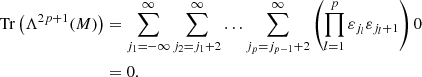
Hence, from Eqs. (B.3), (B.16) and (B.17), and from the fact that Tr(Λ0(M)) = 1 (Simon 2005), we now find Eq. (17):
![$$ \begin{aligned} \Delta = 1 + \displaystyle \sum _{n=1}^{\infty } \left[ \displaystyle \sum _{j_1 = - \infty }^{\infty } \displaystyle \sum _{j_2 = j_1 + 2}^{\infty } \ldots \displaystyle \sum _{j_n = j_{n-1} + 2}^{\infty } \left( \displaystyle \prod _{l=1}^n \varepsilon _{j_l} \varepsilon _{j_l +1} \right) \right]. \end{aligned} $$](/articles/aa/full_html/2021/06/aa40534-21/aa40534-21-eq117.gif)
Appendix C: Deriving solutions for G1, G2 and G3
In this appendix, we show how to derive the solutions to the temporal functions G1, G2 and G3. We recall the equations of interest to this matter, Eqs. (1)–(3), (19)–(21) and (27) for the reader’s convenience:

We recall Eq. (A.4) from Appendix A:
![$$ \begin{aligned} \omega _0 V_0 \sin \left( \omega _0 t \right) \left( \nabla \cdot \boldsymbol{\xi }\right) \boldsymbol{1}_z + \displaystyle \frac{\mathrm{D}^2 \boldsymbol{\xi }}{\mathrm{D}t^2} =&\frac{-1}{\rho _0} \nabla P_1\nonumber \\&+ i k_z { v}_{\rm A}^2 \left[- \boldsymbol{1}_z \left( \nabla \cdot \boldsymbol{\xi }\right) + i k_z \boldsymbol{\xi } \right] . \end{aligned} $$](/articles/aa/full_html/2021/06/aa40534-21/aa40534-21-eq125.gif)
Replacing hi(t) by their definition Gi(t)g(t) for every i ∈ {1, 2, 3} (where  ) and inserting Eqs. (C.4)–(C.7) into the x-component, y-component and z-component of Eq. (C.8), we find that the following equations have to hold:
![$$ \begin{aligned}&\displaystyle \frac{\mathrm{d}^2 G_1(t)}{\mathrm{d}t^2} + K^2 \left({ v}_{\rm A}^2 + { v}_{\rm s}^2 \right) G(t) + k_z^2 { v}_{\rm A}^2 \left[ G_1(t) - G_3(t) \right] = 0, \end{aligned} $$](/articles/aa/full_html/2021/06/aa40534-21/aa40534-21-eq127.gif)
![$$ \begin{aligned}&\displaystyle \frac{\mathrm{d}^2 G_2(t)}{\mathrm{d}t^2} + K^2 \left({ v}_{\rm A}^2 + { v}_{\rm s}^2 \right) G(t) + k_z^2 { v}_{\rm A}^2 \left[ G_2(t) - G_3(t) \right] = 0, \end{aligned} $$](/articles/aa/full_html/2021/06/aa40534-21/aa40534-21-eq128.gif)
with  .
.
We see that G1 and G2 obey the same differential equation and that they thus have the same general solution. They depend on G3, which by solving Eq. (C.11) can be found to be equal to
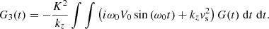
We recall that we defined τ = ω0t. So, since  , we find that
where we used Eq. (13) to find the second equality.
Now, solving Eq. (C.9), we find that
![$$ \begin{aligned} G_1(t)&= \displaystyle \frac{1}{k_z { v}_{\rm A}} \Bigg \{ \cos \left( k_z { v}_{\rm A} t \right)\nonumber \\&\quad \times \left[ \displaystyle \int \sin \left( k_z { v}_{\rm A} t \right) \left( K^2 \left( { v}_{\rm A}^2 + { v}_{\rm s}^2 \right) G(t) - k_z^2 { v}_{\rm A}^2 G_3(t) \right) \mathrm{d}t \right]\nonumber \\&\qquad \quad -\sin \left( k_z { v}_{\rm A} t \right)\nonumber \\&\quad \times \left[ \displaystyle \int \cos \left( k_z { v}_{\rm A} t \right) \left( K^2 \left( { v}_{\rm A}^2 + { v}_{\rm s}^2 \right) G(t) - k_z^2 { v}_{\rm A}^2 G_3(t) \right) \mathrm{d}t \right] \Bigg \} . \end{aligned} $$](/articles/aa/full_html/2021/06/aa40534-21/aa40534-21-eq134.gif)
Having derived expression (C.13), we can also work out Eq. (C.14) and find the following solution for G1:
Analogously,

All Tables
All Figures
|
Fig. 1. Sketch of a longitudinal cut along the axis of a coronal loop harboring a fundamental standing slow body sausage mode, at the velocity’s maximal amplitude (left) and the local cartesian model at the boundary (right). The arrows on the left represent the velocity field and their lengths are to scale with the relative local magnitude of the field for a slow body sausage mode at a given time. The lengths and directions of the magnetic field arrows on the right figure are consistent for that same slow mode, whereas for the velocity arrows only the direction is consistent (the length of the exterior velocity arrow having been increased for visual clarification). |
| In the text | |
|
Fig. 2. Stability diagram of the Mathieu equation. The white zones represent regions of the parameter space where the solution is stable, whereas the gray zones represent regions of the parameter space where the solution is unstable. |
| In the text | |
Current usage metrics show cumulative count of Article Views (full-text article views including HTML views, PDF and ePub downloads, according to the available data) and Abstracts Views on Vision4Press platform.
Data correspond to usage on the plateform after 2015. The current usage metrics is available 48-96 hours after online publication and is updated daily on week days.
Initial download of the metrics may take a while.