| Issue |
A&A
Volume 650, June 2021
Parker Solar Probe: Ushering a new frontier in space exploration
|
|
|---|---|---|
| Article Number | A28 | |
| Number of page(s) | 10 | |
| Section | Planets and planetary systems | |
| DOI | https://doi.org/10.1051/0004-6361/202039284 | |
| Published online | 02 June 2021 | |
PSP/WISPR observations of dust density depletion near the Sun
I. Remote observations to 8 R⊙ from an observer between 0.13 and 0.35 AU
Space Science Division, U.S. Naval Research Laboratory,
Washington,
DC
20375, USA
e-mail: This email address is being protected from spambots. You need JavaScript enabled to view it.
Received:
28
August
2020
Accepted:
3
November
2020
Abstract
Context. In 1929, Russell predicted that dust particles cannot survive in a region close to any star, hence giving justification for a dust free zone to exist inside a certain distance from the star. This theoretical prediction has not been confirmed, even with our Sun.
Aims. We use the unique vantage points and new perspectives of the Parker Solar Probe (PSP) mission to study the dust environment close to the Sun with imaging observations from the Wide Field Imager for Solar Probe (WISPR) as PSP orbits, progressively closer to the Sun (PSP will ultimately reach a perihelion distance of 9.86 R⊙).
Methods. We analyze the radial brightness profile of the axis of symmetry of the F-corona in the WISPR images obtained from heliocentric distances between about 0.350 AU (75 R⊙) and 0.129 AU (28 R⊙) to detect any change from earlier observations. Historically, at observer locations between 1 and 0.3 AU, the brightness of the axis of symmetry has been shown to fall off as a power law of solar distance, r−n, with an exponent of n = 2.3.
Results. We show that as PSP approaches its perihelion distance of 28 R⊙ (orbits 4 and 5), the radial gradient of the brightness profile of the axis of symmetry of the F-corona gradually becomes less steep, starting at about 19 R⊙ down to the shortest elongations reached with current WISPR observations at about 7.65 R⊙. This observational signature is modeled with an ad hoc homogeneous dust density model (i.e., it is not based on any physical model) along the symmetry axis of the zodiacal dust cloud, which (1) varies as the historical density profile, r−1.3, down to 19 R⊙, then (2) stays approximately constant down to 10 R⊙, and finally (3) decreases exponentially to become zero at 3 R⊙. The density profile below 19 R⊙ is accomplished by using a multiplier on the historical density profile that decreases linearly down to 3 R⊙. The distance dependence and range of the multiplier were chosen to best match the brightness observations below 30 R⊙.
Conclusions. The observed brightness decrease in the axis of symmetry is interpreted as the signature of the existence of a dust density depletion zone between about 19 R⊙ and 3 R⊙, which at the inner limit of WISPR’s field of view of 7.65 R⊙ has a dust density that is ~5% lower than the density at 19 R⊙, instead of the expected density which is three times if no depletion zone exists. No noticeable variations in the brightness of the F-corona axis of symmetry were observed from 2018 to 2020.
Key words: methods: data analysis / zodiacal dust / interplanetary medium
© ESO 2021
1 Introduction
The zodiacal dust cloud (ZDC) consists of the dust particles that are in orbit around the Sun, which fill the inner interplanetary space in the Solar System. These dust particles both scatter the photospheric light and emit thermal radiation. The integration of the scattered light along all the lines of sight (LOS) in the field of view (FOV) of an observer at a given location form what is called the zodiacal light. At short elongations, the zodiacal light receives the name of F-corona (F stands for Fraunhofer due to the presence of the photospheric Fraunhofer lines in the visible light spectrum of the F-corona).
Measurements of the zodiacal light have been remarkably stable (Leinert et al. 1982). From observations obtained from 0.3 to 1.0 AU with the Zodiacal Light Experiment (ZLE, Leinert et al. 1975) onboard the Helios mission (Porsche 1981), Leinert et al. (1981) established that the white-light brightness along the symmetry axis of the ZDC follows a power law function r−n with an exponent of n = 2.3 (r being the elongation of the LOS expressed in solar radii, R⊙). By combining many different observations of the F-corona and zodiacal light, Koutchmy & Lamy (1985) developed a model of the zodiacal light between 5 R⊙ and 100 R⊙ with a similar functional form but with an exponent of 2.25. Recently, Stenborg & Howard (2017), in an analysis of the Sun Earth Connection Coronal and Heliospheric Investigation Heliospheric Imager-1A (SECCHI/HI-1A, Howard et al. 2008; Eyles et al. 2009) on the STEREO mission (Kaiser et al. 2008), found that the radial dependence of the brightness along the photometric symmetry axis of the images (i.e., between 4° and 24° elongation) for more than 6 yr of observations exhibits the same functional form, but with an exponent that varies between 2.31 to 2.35, depending on the ecliptic longitude of the observer. Additionally, they found that the center of symmetry of the dust cloud was not at the center of the Sun but shifted toward the barycenter of the Solar System, essentially at about 1 R⊙ in the direction of the average location of Jupiter.
In an analysis of the zodiacal dust in the infrared, Kelsall et al. (1998), for example, modeled the observations from the COsmic Background Explorer (COBE) mission (Mather 1993). Their model included a smooth dust cloud, three asteroidal dust bands, and a circumsolar ring near 1 AU. In particular, they found that the brightness of the smooth component in the inner heliosphere exhibits a radial dependence with a similar functional form as that from the optical observations with an exponent of 2.34, which is remarkably similar to the optical results.
On August 12, 2018 the Parker Solar Probe (PSP) mission (Fox et al. 2016) was launched to explore the inner heliosphere, making fundamental measurements of the solar wind and solar corona from distances that had never been reached before by any man-made spacecraft (S/C). The PSP S/C uses gravity assists from Venus to change the orbital characteristics and systematically lower the perihelion heliocentric distance, such that by December 2024 it will be at 9.86 R⊙ (0.046 AU). WISPR (Wide-field Imager for Parker Solar Probe, Vourlidas et al. 2016) is the only remote sensing suite of the mission, and it is designed to observe the global solar corona in visible light. The WISPR suite consists of two heliospheric imagers, which together image a 40° vertical swath of the solar corona from 13.5° out to 108° from Sun center.
Howard et al. (2019) report on the first results from WISPR, after PSP completed the first two orbits. In that work, they show that the brightness profiles along the symmetry axis exhibited a decrease from what had been expected at elongations below about 20 R⊙ (i.e., a noticeable departure at short elongations from a power law r−n with n ≈ 2.3). Unlike Helios observations, which were obtained from a distance beyond 0.3 AU, WISPR observations during the first two encounters were made from heliocentric distances between about 0.25 AU (54 R⊙) and 0.16 AU (36 R⊙), the latter corresponding to the perihelion of the first two orbits. At this perihelion distance, the inner FOV of the inner telescope reached elongations equivalent to 10 R⊙. They interpreted the decrease to be due to a depletion in the dust density at short elongations.
Russell (1929) predicted that there would be a dust free zone (DFZ) around the Sun caused by the drifting of particles toward the Sun and concluded that such particles would vaporize rapidly once their surface temperature rose above 2000 K. Mann et al. (2004) gave a nice summary of various possible mechanisms for dust depletion and the generation of circumsolar dust bands associated with the sublimation of particles. For instance, Mukai & Schwehm (1981) showed that the collisional heating of dust grains by solar energetic particles and the subsequent erosion by sputtering ejection would be another mechanism for mass erosion, which then could sublimate by thermal radiation at heliocentric distances inside of about 20 R⊙. Rotational bursting has also been identified as a mechanism for disintegrating larger particles into smaller ones, which are then sublimated (Misconi 1993).
In this work, we follow up on Howard et al. (2019) and exploit the WISPR data from the first five orbits completed by PSP at the time of writing this paper, the last two having reached a perihelion distance of ~28 R⊙ (~0.129 AU) on 2020 January 29 and 2020 June 7, respectively, after a Venus gravity assist on 2019 December 26 (the third of a series of seven scheduled until the end of the nominal science mission at orbit 24 in 2025; after the seventh gravity assist, the aphelion of the PSP orbit will be inside the orbit of Venus). The first three orbits reached a perihelion distance of ~36 R⊙ (~0.165 AU) on 2018 November 6, 2019 April 4, and 2019 September 1, respectively.
The rest of this paper is organized as follows. In Sect. 2, we briefly describe the WISPR instrument and observationsused, along with a detailed description of the methodology employed and measurements obtained (Sects. 2.1 and 2.2). Then, we characterize the measurements by means of (1) an ad-hoc empirical model (Sect. 3.1), and (2) forward modeling at short elongations to help interpret the observational results (Sect. 3.2). Our results and interpretation are discussed and put into context in Sect. 4. Finally, we conclude in Sect. 5.
2 Observations and methods
WISPR is a visible light instrument consisting of two telescopes that image the photospheric light scattered by both the dust in the ZDC and the free electrons streaming away from the Sun in the solar wind. The images also reveal the star field, planets, other solar system objects, such as comets or features such as cometary or asteroid dust trails (e.g., Battams et al. 2020), and extended galactic sources. A comprehensive description of the instrumental details is given in Vourlidas et al. (2016). Briefly, the FOV of the two WISPR telescopes (hereafter WISPR-I and WISPR-O) cover the interplanetary medium between 13.5° and 53.58° as well as 50° and 108° elongation, respectively. The imaging data are recorded by an active pixel sensor (APS) 1920 × 2048 pixel2 detector on each telescope. The filter passbands of WISPR-I and WISPR-O are 490–740 nm and 475–725 nm, respectively. For WISPR, thenominal science data acquisition is primarily carried out during the so-called solar encounters, which nominally occur when PSP is below 0.25 AU. During some orbits (i.e., when the geometrical configuration of Earth and PSP permits additional telemetry), the observing period gets extended to heliocentric distances greater than the nominal 0.25 AU (i.e., extended science windows).
To characterize the radial evolution of the F-corona brightness profile along its symmetry axis, we used WISPR Level-2 (i.e., calibrated) data (hereafter L2, Hess et al., in prep.) acquired during the first five solar encounters, excluding encounter 3. If WISPR observations exist, the analysis is extended to data sets obtained from up to 0.35 AU. Orbit 3 data are excluded from the analysis because, unfortunately, WISPR-I data science products obtained during a large part of the nominal encounter in this orbit (i.e., 2019 September 1–2019 September 8) were corrupted and hence unusable. In Table 1 we show the time window of each set used and the respective location of the PSP S/C.
The calibration procedure (Hess et al., in prep.) consists of the removal of instrumental effects, such as detector bias and optical vignetting, and the conversion of the signal from digital numbers (DN) to units of mean solar brightness (MSB). In these units, the brightness is compared to the average brightness of the solar disk,  (i.e.,
  ; Leinert et al. 1998) and is the traditional unit1 used in observations of the solar corona. In spite of the constantly changing radial distance of PSP, the MSB units used for WISPR actually represent the brightness compared to the brightness of the Sun on the WISPR detectors as if they were at 1 AU. Therefore, using MSB units enables easy cross-calibration with other space borne imagers near Earth’s orbit such as SOHO/LASCO (Brueckner et al. 1995) and STEREO/SECCHI.
The key factor in converting the raw (Level-1) images (normalized by the exposure time) from DN s−1 to MSB (Hess et al., in prep.) is the calibration factor, CMSB, which is defined as
 (1)
(1)
where D⊙ is the angular size of the Sun (32 arc min), Dpix is the angular pixel size, which equals 1.712 arc min (1.262 arc min) for an unbinned WISPR-I (WISPR-O) image, and I⊙ is the solar intensity, calculated by integrating the solar flux over the instrument bandpass. While this allows for a theoretical explanation for the calibration factor, it is actually determined using stars with known stellar spectra observed by the WISPR detectors and comparing it to the observed signal based on aperture photometry. These same stellar sources have also been used to update the geometric distortion and pointing information for each image, improving the accuracy of converting pixel coordinates in the image to physical coordinates in the heliosphere.
Observing time window of the observation samples used.
2.1 Geometric determination of the symmetry axis
The scene in WISPR calibrated images is dominated by photospheric light scattered by the dust particles in orbit around the Sun (F-corona). The contribution of Thomson scattering by the free electrons (K-corona) amounts to only a few percent (only relevant along bright streamers), which contributes to the variability in the measurements (see Sects. 3.1.1 and 3.1.2).
The WISPR images exhibit a well-defined axis of symmetry, which arises from the 2D projection of the warped plane that divides the northern and southern portions of the ZDC; when the ZDC is seen edge-on, this warped plane is the surface of symmetry of the ZDC. Occasionally, coronal structures, such as streamers or bright coronal mass ejections, can distort the axis in a specific region of the image. This hindrance does not affect the analyses, but it introduces an error (see Sect. 3.1.1).
For illustration purposes, we display a typical WISPR-I calibrated image in Fig. 1. The nose of the iso-contours outlines the symmetry axis of the F-corona, which is delineated with the white dashed line. In this image, a coronal streamer slightly affects the F-coronal brightness at short elongations; however, at greater heliocentric distances, the streamer’s brightness decreases faster than the F-corona and hence, there is less distortion. Also at the edges of the image, the contours exhibit an odd behavior. This is due to reflections from the edges of the protective cover on the detector. Therefore, to avoid having the measurements affected by border effects in our analyses, we have excluded the columns to the left of the innermost vertical dashed line (at Col. # 63) and to the right of the outermost vertical dashed line (at Col. # 950). The determination of the symmetry axis is not affected by the reflections at the top and bottom of the image.
The axis of symmetry of the F-corona on the image plane is simply defined as the line traced along the pixel locations [xi, yi] where the brightness peaks at each column xi. In other words, yi = max[B(xi)], where the letter B denotes the brightness2. The majority of WISPR-I data acquired during orbits 1, 4, and 5 were down-linked 2 × 2 binned (i.e., half resolution); therefore, i ranges from 0 to 959, while for orbit 2 they were downlinked at full resolution. As for WISPR-O, all the data sets were downlinked at half resolution. Therefore, for the purposes of our analysis, all WISPR-I images from orbit 2 were downsized to half of the resolution of the detectors.
Then, to avoid imposing any assumption on the shape of the symmetry axis of the brightness of the images while minimizing the presenceof outliers, we applied a robust nonparametric algorithm to model the shape of the symmetry axis. The outliers are spurious signals resulting from the presence of bright objects (e.g, point-like sources, such as a planet or star, or bright portions of extended objects, such as the Milky Way). Thus, the radial evolution of the symmetry axis was fitted in detector coordinates with a nonparametric regression algorithm to avoid invoking an analytical function (LOWESS algorithm, short for “locally weighted scatterplot smoothing”, Cleveland 1979).
Figure 2 shows, the brightness profiles of the symmetry axis for a sample of WISPR-I images on each one of the four data sets employed in this work as a function of elongation in solar radii in a log-log representation (in black color on each panel). The sampling was done by selecting images in the time range specified in Table 1 spaced by about 5° S/C longitude. The selected images were those taken when the S/C longitude L at the time of the observation was closest to Lk = k * 5 + 35° with k = 0, 1, 2, ..., 35. As a result of this choice, the size Nj of each sample (j denotes the encounter) is as follows: N1 = 31, N2 = 39, N4 = 44, and N5 = 43.
Each telescope of the WISPR instrument suite has a fixed FOV and thus always observes the same range of elongations from the pointing axis of the PSP S/C. Thus, when the S/C is pointed at the Sun (i.e., its nominal attitude), the inner FOV of WISPR-I starts at 13.5° from Sun center and extends to 53.5°. However, due to the PSP highly elliptic orbit, the angular size of the Sun strongly depends on the heliocentric distance of PSP. For example, the angular size of the Sun is 1.52° at 0.35 AU and 4.12° deg at 0.129 AU. For comparison purposes, at 1 AU, the angular size of the Sun is 0.54°. Therefore, the fixed angular FOV comprises different heliocentric distances as PSP moves along its orbit. To reflect this in Fig. 2, as well as in the rest of the figures in this work, we converted the elongation of each pixel along the symmetry axis (in degrees) to an equivalent elongation expressed as heliocentric distance (in solar radii). The conversion was carried out by normalizing the corresponding elongation of any given pixel by the apparent radius of the Sun (expressed in degrees) at the time of the observation3.
The seamless overlapping of the WISPR-I brightness profiles on each data set observed in Fig. 2 indicates that the stray light for WISPR-I at these heliocentric distances is negligible. We also notice that the combination of all the brightness profiles for any given data set look linear beyond about 20 R⊙. Therefore, we robust-fit a linear model to each sample restricting the elongation to be ϵ ≥ 20 R⊙ (i.e., beyond the vertical red dashed line). The models obtained are overplotted in a red color. Their coefficients (with their standard deviations in parenthesis) are given in Table 2. It is important to notice that the plots in Fig. 2 clearly show the shorter elongation distances covered in orbits 4 and 5 (~ 7.65 R⊙ compared to ~ 10 R⊙). These observations expand on an earlier report (Howard et al. 2019), for which the lowest distance was 10 R⊙.
Similar plots for the brightness profiles obtained from corresponding WISPR-O images are shown in Fig. 3 (in this case, the size of each sample is N1 = 29, N2 = 36, N4 = 44, and N5 = 39). Unlike the brightness profiles from WISPR-I, the ones from WISPR-O for any given orbit do not match. We attribute this to an additive brightness term, which hereafter we simply refer to as stray light.
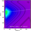 |
Fig. 1 WISPR-I calibrated image taken during the nominal science encounter in orbit 1. The image is displayed in false colors, with iso-contours in a darker color tone, to illustrate the shape of the F-corona and the location of its symmetry axis (dashed white line across the noses of the iso-contours). For details, see the text. |
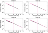 |
Fig. 2 Brightness profiles of the symmetry axis of the F-corona in WISPR-I calibrated images. A robust linear model, as obtained from elongations ϵ ≥ 20 R⊙, has been fitted (in red) to each data set (the coefficients of the models are reported in Table 2). |
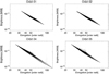 |
Fig. 3 Brightness profile of the symmetry axis of the F-corona in WISPR-O calibrated images, which were not corrected by stray light. |
2.2 WISPR-O stray-light correction
The determination of the contribution of the stray-light level is a necessary step in the calibration of any white-light coronagraph or heliospheric imager. For the purposes of this work, the term “stray light” comprises instrumental stray light and diffuse galactic background.The traditional method to compute the overall level of the unwanted sources (e.g., Bohlin et al. 1971) is to match the slope to previous measurements by subtracting a single number from the entire image. Since WISPR has two telescopes with a small overlap between them, an additional constraint is that the data from WISPR-I (40° FOV) and WISPR-O (50° FOV) must match in the region of overlap. Previous measurements of the zodiacal light in this region from the Helios spacecraft (e.g., Leinert et al. 1981) and for the STEREO spacecraft (Stenborg et al. 2018) have found that a log–log plot of brightness versus heliocentric distance is linear with a slope of about −2.3 for the heliocentric distances of the observer varying from 0.3 to 1 AU and at the line of nodes of the ZDC.
The choice of a constant term is due to the nature of the stray light sources, namely photospheric light diffracted by the baffle edges and the diffuse galactic background. Direct sunlight is blocked by the forward baffles, but some light is diffracted by the edges of the baffles. The intensity of this light is much less, but it is still significant and illuminates the front surface of the first lens, which causes scattering within the body of the lens. This scattered light exits the back surface of the lens as a uniform source illuminating the entire detector more or less equally. The diffuse galactic background is simply a constant value.
Therefore, to determine the stray-light level, we simply followed Bohlin et al. (1971) and found the value that makes the brightness profiles of the WISPR-O images (Fig. 3) match the linear model of the corresponding WISPR-I data set (Fig. 2). Since the uncorrected WISPR-I profiles are already linear, the stray light correction only applies to the WISPR-O images4. The diffraction component increases with decreasing PSP heliocentric distance; therefore, the stray light correction depends on the observer’s distance and hence was computed for each individual WISPR-O observation.
The results are shown in Fig. 4, which displays the combined WISPR-I (in black) and WISPR-O (in green) profiles after stray-light correction (each data set in a different panel). The red, dashed linesshow the robust linear fitting to the combined data sets as obtained considering elongations ϵ ≥ 20 R⊙ (the coefficients of the models are shown in Table 3).
Figure 4 clearly shows the linear nature of the dependence of log(B) with log(r) above about 20 R⊙ and the departure from linearity below that distance. The photometric stability of the two instruments (the orbits under analysis occurred over a period of 18 months) is evidenced by the overlapping profiles within each orbit, the similarity of the linear models among the different orbits, and the very low standard deviations reported in Table 3. In Sect. 3.1.1we address the causes that lead to the small variations between the coefficients corresponding to the different orbits.
 |
Fig. 4 Brightness profile of the symmetry axis of the F-corona in the FOV of WISPR-I and WISPR-O calibrated (and stray-light corrected) images. A robust linear model, as obtained from elongations ϵ ≥ 20 R⊙, has been fitted (in red) to each data set (the coefficients of the models are reported in Table 3). |
3 Modeling of the F-corona brightness profile along its symmetry axis
3.1 Empirical modeling
To model the brightness profile of the F-corona along its symmetry axis, we first generated an empirical model of the observed brightness profile using the combined WISPR-I and WISPR-O data and considering all four orbits together. Figure 5 displays all the brightness profiles without a distinction for the observation time. As already noticed in Figs. 2 and 4 for the profiles on each particular orbit, they also all align well when the four orbits are considered together.
Therefore, to reproduce both the linear shape of the profile at large elongations and the exponential decay at short elongations, we propose an ad-hoc empirical model (hereafter BM) with the following functional form:
 (2)
(2)
where x denotes the elongation expressed in R⊙ and Ai (i = 0−4) are the free parameters of the model, which are estimated via a robust-fitting to the data in Fig. 5. The red dashed line delineates the resulting model BM (A0 = −0.256, A1 = 1.071, A2 = 6.143, A3 = −7.413, A4 = −2.286), and the dashed light-blue line is its linear part extrapolated to 7 R⊙ (i.e.,  ). The verticalred and blue dashed lines depict the shortest elongations observed during orbits 4 and 5, and 1 and 2, respectively. A comparison of the coefficients for the linear part of the BM model with the coefficients of the linear fits to the data above 20 R⊙ (Table 3) demonstrates that the addition of the exponential term does not significantly affect the coefficients of the linear terms (i.e., the slope and intercept).
The inset in Fig. 5 displays the relative decrease in the signal at short elongations (i.e., between about 7 R⊙ and 25 R⊙) compared to what is expected if no depletion zone exists. We note that at the shortest elongation covered (7.65 R⊙), a decrease of almost 35% exists.
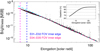 |
Fig. 5 Combined brightness profiles of the symmetry axis of the F-corona in WISPR-I and WISPR-O calibrated images. The empirical model BM is delineated by the red dashed line. The light-blue dashed line depicts the linear portion of the empirical model extrapolatedto 7 R⊙. The inset displays the departure of BM from the linear trend. |
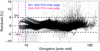 |
Fig. 6 Residuals of the sampled measurements in orbits 1, 2, 4, and 5 with respect to the empirical model BM. See the text for a discussion. |
3.1.1 Residuals
As shown in Fig. 5, the brightness profiles computed for the four different orbits from a variety of observer distances (delineated by black dots) match each other rather well. Likewise, the agreement between the empirical model (red dashed line) and the data is also rather good. In this section, we are going to quantify the predicate “rather”.
As is always the case, a model of a natural phenomenon is just a model and hence, the reproduction of the observations and measurements is not perfect. Our empirical model, in particular, is just an ad-hoc model, which was chosen without any physics behind it. It is not intended to explain what causes the observed behavior but to just help us discriminate locally generated phenomena that might contaminate our measurements. In particular, our empirical model is described by a monotonic function aimed at reproducing the monotonic aspect of the smooth component of the zodiacal (F-corona) light. Thus, it is well suited to help discriminate inhomogeneities in the measurements.
Figure 6 shows the percentage error (i.e., the residuals) between the empirical model and the data5. We notice that the mismatch is between 5 and −4%. The downward excursions beyond −4% at elongations ϵ ≲ 20 R⊙ and 30 R⊙≲ ϵ ≲ 55 R⊙ correspond to the “barbs" in the brightness profiles observed during orbits 4 and 5, which result from saturation at the inner edge of the WISPR-I and WISPR-O detectors, respectively. On the other hand, the “cloud” of dots observed above 5% that starts to be discernible at ~ 30 R⊙ and continues up to ~ 80 R⊙ results from the passage of the Milky Way and its denser star field, its effect being more noticeable in the FOV of WISPR-O, where the F-corona brightness is lower. There are also other outliers from the general trend, which are due to transits of bright objects suchas stars and planets.
At the largest scale, the residuals show, on average, no trend with a 0% median level. At shorter scales in particular, they exhibit, however, a wiggly aspect that indicates that the empirical model is only right within [−4%,+5%] accuracy. This most probably results from locally generated phenomena and/or from the temporal differences between the orbits. In that regard, we would like to draw attention to the splitting observed at short elongations, which is an observational finding that we address next.
3.1.2 Orbital variations
To explore, in more detail, small deviations between the model and the observations and to help us identify possible locally generated phenomena, we now address the analysis of the residuals for each orbit separately, discriminating different portions of the orbits. The residuals grouped per orbit are shown in the four panels of Fig. 7. In the figure, we can notice similarities and differences between them. As mentioned above, “the barbs” are only seen in orbits 4 and 5 (both detectors). In addition, all of them show a relatively larger increase starting at about 50 R⊙, which is caused by the passage of the Milky Way through WISPR-O (the residuals are larger at the longest elongations because of the relative contribution of the contaminating signal of the Milky Way to the zodiacal light signal).
Another interesting common feature is the relative minimum of the residuals near 15 R⊙ (which is pointed out with the vertical dashed line). This might be indicative of a necessary adjustment to the functional form of the empirical model to better follow the overall trend of the brightness profile, but this is beyond the objectives of this work.
Orbits 4 and 5 show a triangular shape centered at about 22 R⊙, which is notnoticeable in orbits 1 and 2. This is due to the crossing of the Milky Way through WISPR-I. It is not seen at the orbits with higher perihelia because the dust column along the LOS in those orbits is slightly longer, and hence the relative contributionof the Milky Way to the F-corona signal is smaller.
Interestingly, Fig. 7 also shows a clear splitting of the residuals in orbits 1, 4, and 5. The splitting also exists in orbit 2 but it is not noticeable at the scale of the plot. For orbits 4 and 5, the splitting occurs at short elongations, starting below ~15 R⊙. On the other hand, orbit 1 exhibits multiple splittings starting at higher elongations. We note that the splitting indicates a brightness departure from the empirically modeled brightness, which smoothly increases toward the Sun.
Since the objective of this work is to characterize the dust density in a region of space close to the Sun (i.e., where the gradient of the zodiacal dust light departs from linear), we concentrate now on the orbital characterization of the splitting of the residuals and their origin. To that aim, we restrict the analysis to measurements derived from WISPR-I observations at elongations ϵ < 17 R⊙. In Fig. 8 we show the corresponding measurements for the four orbits under study, with the profiles grouped by color depending upon the location of the observer. The color coding is indicated in Table 4 (the respective locations of the observer at the edges of each interval are indicated in the Heliocentric Aries Ecliptic or HAE system).
Figure 8 shows that the splitting is a transient effect, varying from orbit to orbit. Therefore, the temporal behavior and relative intensity (below 5% of the expected F-corona component) of these observational signatures suggest they are due to the projection in the plane of the sky of K-corona structures (e.g., streamers) that pass over the projection of the symmetry plane of the ZDC as the sequence of observations develop. We emphasize that the measurements have not been filtered or interpolated; the only processing that has occurred has been calibration. Close inspection of the WISPR-I data confirms this conjecture.
 |
Fig. 7 Residuals of the sampled measurements with respect to the empirical model BM grouped by orbit. See the text for a discussion. |
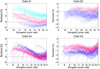 |
Fig. 8 Residuals restricted to WISPR-I sampled profiles at ϵ < 17 R⊙. The different colors indicate the observer’s location; see Table 4. |
3.2 Forward modeling of the brightness profile in the depletion zone
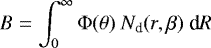
The observed white-light brightness of an optically thin structure and medium in the corona results from the integration along the LOS of the photospheric light scattered by the different elements along the integration path. The scattering processes depend, to first approximation, on the size of the particles with respect to the wavelength of the incident light. Therefore, for a given particle population, the brightness B can be estimated using
 (3)
(3)
where Φ(θ) represents the scattering function for that type of particle at the scattering angle, θ, and Nd is the particle density at the heliocentric distance, r, and angle from a given plane, β. The integration is to be performed over the LOS, dR, from the observer’s location up to infinity.
Motivated by the unprecedented imaging of the white light coronagraph instruments (LASCO, Brueckner et al. 1995) on board the Solar and Heliospheric Observatory (SOHO, Domingo et al. 1995) mission, Thernisien & Howard (2006) developed a program to perform the integration along any given LOS of a model of the electron density of any given coronal structure using Thomson scattering. The algorithm allows the user to place the coronal structures at different locations along the LOS. In that original work, they focused on the modeling of the three-dimensional nature of a coronal streamer as observed with the SOHO/LASCO coronagraphs. The code was then used to model coronal mass ejections (e.g., Thernisien et al. 2006) assuming a graduated cylindrical shell (GCS) model - a density analog of a magnetic flux rope. The program, RAYTRACE, and a user manual have been deposited in the SolarSoft system library (Freeland & Handy 1998) under the STEREO/SECCHI tree and are publicly available (Thernisien et al. 2011).
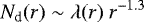
In brief, to model the observed white-light brightness, RAYTRACE needs (1) a density distribution along the LOS and (2) a volume scattering function. For the modeling of the zodiacal light, several dust density models have been proposed (see, e.g., Giese & Kinateder 1986; Misconi & Rusk 1987). The main difference among these models resides in the radial and latitudinal dependency of the density distribution. In particular, for this work, we have taken the dust density model proposed by Leinert et al. (1976) as a baseline, which is best suited for small inclinations (our case), namely,
 (4)
(4)
where r denotes the heliocentric distance of the dust element along the LOS contributing to the total brightness observed and β, its latitudinal displacement from the symmetry plane of the ZDC. For this study, we set β to be zero for the following reason: the PSP orbital plane is, at maximum displacement, below ± 0.8° from the symmetry plane of the ZDC during orbits 1 and 2, and below ± 0.1° during orbits 4 and 5; therefore, WISPR is essentially observing the symmetry plane of the ZDC edge-on. If our assumption is incorrect, then a dependence of the slope with the location of the observer should have been noticeable (see, e.g., Stenborg et al. 2018). As shown in Sect. 2.1 (see Fig. 2), the seamless superposition of the brightness profiles from WISPR-I that were obtained in four different orbits, each comprising an extended longitudinal range of more than 180° (see Table 1; orbit 1 is the exception as it only comprises observations from a 144° longitudinal range), effectively shows that if any dependence exists, its effect is within the error of our measurements.
For the empirical volume scattering function (VSF), we used the VSF of Lamy & Perrin (1986), which incorporates the physics of the scattering process with an ensemble of particle sizes and indices of refraction into a single empirical function. The VSF is a function only of the scattering angle θ, that is, VSF = Φ(θ), so that only the density distribution of particles needs to be provided to determine the brightness at any given LOS elongation. The choice of this VSF (and density model described above) was motivated by its use in reproducing the brightness observations performed by the ZLE on the Helios mission (Lamy & Perrin 1986).
In our implementation of RAYTRACE in solving the integration in Eq. (3), we set the upper integration limit to 2 AU instead of infinity for simplicity purposes. This choice was mainly motivated by the closeness of the observer to the Sun (the dust density model is peaked at the Sun). The error due to this truncation is lower than 3%, which is within the error of our measurements.
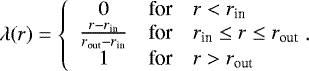
Our analyses of the brightness profiles (Sect. 2.2) show that below about 20 R⊙, the radial gradient gets shallower down to the inner limit of WISPR-I of 7.65 R⊙. We conjecture that this change is due to the existence of a zone where the dust gradually depletes, which we call a dust depletion zone (DDZ). Therefore, to account for this gradient change, we used a depletion factor (i.e, a multiplier) for the density given in Eq. (4), which we set to vary linearly from 0 to 1 within a restricted heliocentric distance range of ([rin, rout]). Thus, the modified density distribution model along the symmetry axis becomes
 (5)
(5)
where λ(r) is a simple function defined as
 (6)
(6)
In Fig. 9 we show the comparison between the empirical model BM (continuous black line) and the simulation run with the forward modeling considering a DDZ between (1) 2 R⊙ and 20 R⊙ (green dashed line), and (2) 3 R⊙ and 19 R⊙ (red dashed line). It is important to note that at the resolution of the plot of both models practically superimpose on each other. In the inset, we display the relative percentage error between the empirical model and the simulations using the same color code. The dashed vertical line at 7.65 R⊙ marks the innermost limit covered by the FOV of WISPR-I in the analysis carried out in this work (in the plot, both models are extrapolated below this distance down to 6 R⊙). In summary, using the VSF developed in Lamy & Perrin (1986) and the modified density distribution for the symmetry axis given by Eqs. (5) and (6), we find the best matching to be between the empirical model BM and the simulated brightness profile for [rin, rout] = [3, 19] R⊙.
The values of both the inner and the outer limit of the DDZ displayed above are empirical parameters. The outer limit is where the slope of the brightness profile in the log–log representation starts to be constant with heliocentric distance (hence the outer edge of the DDZ). The value of these two parameters was determined by minimizing the difference between theempirical model defined by Eq. (2) and the forward modeling of the brightness down to 7.65 R⊙. As such, they define the hypothetical extent of a DDZ under the ad hoc assumption of a dust density model defined by Eq. (5) (with the simple linear multiplier λr defined by Eq. (6)). We note that the upper limit of the DDZ near 19 R⊙ is an observational fact. However, the computed inner limit is beyond the limit of our observations and hence cannot be supported with direct observational evidence.
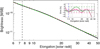 |
Fig. 9 Comparison between the empirical model (in black color) and the forward modelingof the zodiacal light along the symmetry axis considering a DDZ between 2–20 R⊙ (in green color) and 3–19 R⊙ (in red color). The inset shows the relative error of the simulations compared to the empirical model (same color code). For details, see the text. |
4 Discussion
The orbital geometry of the PSP S/C enables the study of space near the Sun from distances that have never been reached before by any man-made S/C. For WISPR, a remote sensing instrument, this provides a unique opportunity to study the dust environment close to the Sun, without the contribution from a large column of dust between the observerand the near-Sun region. This allowed us to detect observational signatures compatible with the existence of a DDZ, a zone that is leading to the eventual DFZ postulated by Russell (1929). A signature of a DDZ had already been identified in the initial WISPR results from the first two PSP orbits by Howard et al. (2019), who then interpreted the decrease in the radial gradient of the brightness profile of the symmetry axis of the F-corona to be due to a decrease in the gradient of the dust density compared to what was expected at larger elongations. Here, we have refined and extended that analysis using PSP orbits 4 and 5, both with perihelia at about 28 R⊙, which allowed us to lower the inner limit of observation from 10 R⊙ to 7.65 R⊙. These extensions permitted a more rigorous and detailed analysis of the DDZ.
The existence of a DDZ has been generally believed to be due to the sublimation of dust particles, which would occur at different solar distances depending on the species and size of the particles (e.g., Belton 1966; Mann et al. 2000; Kobayashi et al. 2009). Moreover, the presence of circumsolar dust rings with density enhancement factors of 1 to 4 has been postulated to exist at the beginning of the region where a species starts to sublimate; however, their presence has not been confirmed from 1 AU yet (see, e.g., Mann et al. 2004, and references therein). As Mann et al. (2004) also discussed, the density of dust particles can also decrease by other processes such as rotational bursting or gradual erosion until the particles are blown away by radiation pressure (e.g., Mukai & Schwehm 1981; Misconi 1993). These two models have predicted the destruction of particles at distances <20 R⊙, which are very suggestive for the WISPR measurements presented in this work.
Our measurements below 20 R⊙ do not show evidence of any discrete enhancements due to the effect of sublimation of the different species as predicted by Kobayashi et al. (2009), for example. This indicates that either a circumsolar dust ring associated with the sublimation of a given species of dust particles does not exist in the DDZ, or it is below the WISPR detection threshold above the local brightness (of about 0.1%). This would imply that processes that produce a relatively smooth decrease in the dust density are more likely to occur, such as the sublimation due to large fluffy dust particles as modeled by Kimura et al. (1997), which if large enough can cause the enhancement to be obscured. It could still be, however, that these dust ring enhancements would manifest below 7.65 R⊙. The next perihelion for PSP (orbit 6) will be at 20 R⊙, which will take the inner FOV of WISPR-I down to about 5 R⊙.
This work benefited from the photometric stability of both WISPR telescopes (see, e.g., Fig. 4). As observed in Fig. 5, the brightness profiles of the symmetry axis of the F-corona appear to (1) be stationary among the different orbits analyzed, (2) be linear down to elongations equivalent to about 19–20 R⊙, and (3) depart from linearity at shorter elongations, their gradient becoming shallower closer to the Sun. The former is supportive of the notion of a constant ZDC (Leinert et al. 1982). The latter, on the other hand, is a signature that has not been observed by any other white light instrument before. Therefore, the question we then tried to answer was whether the gradual, relative diminishing of the white light signal along the symmetry axis observed at short elongations does indeed correspond to a signature of a DDZ.
To answer this question, we first modeled the trend of the brightness observed in a log(B) −log(r) space by proposing a monotonic function consisting of the sum of an exponential and a linear function. This model allowed us to determine the contamination of the signal due to the presence of discrete K-corona structures (Sect. 3.1). We found that the coronal electron structures contribute to a maximum of 5% of the F-corona signal, hence the accuracy of the ad-hoc, empirical model in describing the brightness profiles of the F-corona.
Then, we simulated (with forward modeling) the zodiacal light brightness along the symmetry axis as described by our empirical model, assuming a dust density model and a volume scattering function that had been used to explain the Helios observations. In the density model, we imposed a multiplier that decreases linearly with heliocentric distance starting at the observed outer boundary of the postulated DDZ to become zero at an empirically-determined distance to match the observations. The latter would be the long-sought outer limit of the DFZ postulated by Russell (1929) if the dust density in this zone decreases in our ad hoc proposed way. The impetus for choosing a linear multiplier to model the dust density decrease was the very uniform decrease in the observed brightness and the absence of discrete drops in the brightness profile. This suggested a continuous process and not a series of discrete events.
A difficulty with the modeling used here is that the empirical VSF was validated from the Helios observations for observer positions from 0.3 to 1.0 AU, and it is thus strictly valid in that interval. In the modeling we have presented in Sect. 3.2, we have assumed that the VSF has not changed for the observer positions from 0.13 AU and greater. Since it embeds the scattering properties of different materials and different particle sizes, these may change at closer distances to the Sun.
In spite of the above mentioned difficulty, we found that our observations can be explained with this simulation by imposing a DDZ between [3–19] R⊙ (Fig. 9). Therefore, the observational signatures detected at short elongations are compatible with the existence of a DDZ. While this decrease could indeed lead to the DFZ, it has not yet led to its detection from the perihelion distances reached so far by PSP. Leinert et al. (1981) searched for signatures that could support the existence of a DFZ in the Helios data but did not see any up to their inner limit of ~20 R⊙ (the limiting distance observable by Helios, Leinert et al. 1978). At 0.3 AU (i.e., at a distance that matches theclosest heliocentric distance reached by Helios), the inner edge of WISPR-I is about 14.6°. Due to the restriction of our analyses to columns beyond Col. 64 in WISPR-I images in particular (see Sect. 2.1), the elongation of the innermost part of the FOV then corresponds to about 17.3° for the observer at 0.3 AU, which in turn is equivalent to about 19.4 R⊙ when normalized by the apparent radius of the Sun in degrees. Therefore, WISPR-I, similarly to HELIOS,did not observe signatures of the DDZ as they only start to clearly manifest below 19 R⊙.
As previously stated, the dust depletion within 19 R⊙ was modeled assuming an ad hoc linear multiplier (Eq. (6)). In Fig. 10 we display the resulting dust density profile (Eq. (5)) normalized to the dust density at the outermost edge of the DDZ zone (blue curve). The shadow areain yellow points out the DDZ, and the red dashed line indicates the innermost distance observed at this time. At the beginning of the DDZ, the dust density model exhibits a sharp transition compared to the smooth evolution of the brightness profile. We note that the smooth brightness profile is due to the smoothing effect of the integration all along the LOS. Below that distance, the dust density follows a slight linear upward trend from 19 R⊙ down to 13 R⊙, where it is about 2.4% larger than at 19 R⊙. This could explain the “negative” depression observed in the plot of the residuals at about 15 R⊙ (Fig. 6). At the WISPR innermost limit of 7.65 R⊙, the resulting dust density is ~5% below the value at 19 R⊙, instead of being ~3× larger than it would have been if the density followed Eq. (5). It is important to note that in order to match the WISPR measurements, we had to impose the beginning of the DFZ at 3 R⊙ (under the assumption of a linear dust density decrease), which is inside the presumed distance of about 4 R⊙ (e.g., Mann et al. 2000).
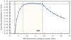 |
Fig. 10 Model of the dust density (Eq. (5)) inside 32 R⊙ relative to the outermost edge of a DDZ between [3–19] R⊙ as modeled assuming a linear density decrease described by Eq. (6). The dashed, vertical line in a red color indicates the innermost distance covered by the WISPR-I images in this study. |
5 Conclusions
The WISPR observations reported here show excellent photometric stability during the observation period of the first five orbits of PSP from2018 to June 2020. We summarize our conclusions as follows:
- 1.
For an observer (PSP) at heliocentric distances between 0.35 and 0.129 AU, the combined brightness profile of the symmetry axis of the images’ brightness as a function of solar distance in a log–log representation is reproduced with an empirical, ad-hoc model consisting of a linear and an exponential term that fit the observations in all their extension within [+5%,−4%].
- 2.
The combined brightness profile is linear down to 19 R⊙, the slope being − 2.289 ± 0.004. This value is within 0.5% of those determined by Helios & STEREO.
- 3.
Below 19 R⊙, the slope decreases smoothly down to the current WISPR inner limit of 7.65 R⊙.
- 4.
The consistency and seamless matching of the brightness profiles of the symmetry axis from 7.65 R⊙ to almost 130 R⊙ for the two years since the PSP launch verifies the constancy of the F-corona. Variations below 30 R⊙ were observed on the order of <5%, which were associated with electron corona structures, such as coronal streamers. Beyond that distance, fluctuations (also below 5%) are explained by the passage of an extended galactic source, that is, the Milky Way.
- 5.
A forward modeling of the F-corona brightness assuming (1) a smooth dust density model that follows r−1.3 and including a DDZ where the density multiplier decreases linearly between 19 R⊙ and 3 R⊙, and (2) an empirical volume scattering function that was proven to reproduce Helios observations, reproduces our brightness measurements with an error of <3% below 35 R⊙. This supports our conjecture that the gradual change of the radial gradient of the F-corona symmetry axis brightness profile is a signature of the existence of a DDZ inside 19 R⊙.
In summary, we have presented observations of the F-corona from an observing platform between about 0.35 and 0.129 AU from the Sun. The brightness signatures observed below about 19 R⊙ are compatible with the existence of a DDZ. However, no evidence of dust banding was detected, probably indicating that the dust remaining at these heights is resistant to pyrolysis and may be similar to quartz or obsidian. We encourage modeling analyses using these data to try to understand the nature of the dust particles in this region. Certainly, by the time that PSP has reached its final perihelion at 9.86 R⊙ (placing the inner limit of WISPR at about 2 R⊙), the DFZ will be revealed.
Acknowledgements
Parker Solar Probe was designed, built, and is now operated by the Johns Hopkins Applied Physics Laboratory as part of NASA’s Living with a Star (LWS) program (contract NNN06AA01C). Support from the LWS management and technical team has played a critical role in the success of the Parker Solar Probe mission. We gratefully acknowledge the efforts and dedication of Nathan Rich in operating the WISPR instrument. This work was supported by the NASA Parker Solar Probe Program Office for the WISPR program (contract NNG11EK11I).
References
- Battams, K., Knight, M. M., Kelley, M. S. P., et al. 2020, ApJS, 246, 64 [Google Scholar]
- Belton, M. J. S. 1966, Science, 151, 35 [Google Scholar]
- Bohlin, J. D., Koomen, M. J., & Tousey, R. 1971, Sol. Phys., 21, 408 [Google Scholar]
- Brueckner, G. E., Howard, R. A., Koomen, M. J., et al. 1995, Sol. Phys., 162, 357 [NASA ADS] [CrossRef] [Google Scholar]
- Cleveland, W. S. 1979, J. Am. Stat. Assoc., 74, 829 [Google Scholar]
- Domingo, V., Fleck, B., & Poland, A. I. 1995, Sol. Phys., 162, 1 [NASA ADS] [CrossRef] [Google Scholar]
- Eyles, C. J., Harrison, R. A., Davis, C. J., et al. 2009, Sol. Phys., 254, 387 [Google Scholar]
- Fox, N. J., Velli, M. C., Bale, S. D., et al. 2016, Space Sci. Rev., 204, 7 [NASA ADS] [CrossRef] [Google Scholar]
- Freeland, S. L., & Handy, B. N. 1998, Sol. Phys., 182, 497 [NASA ADS] [CrossRef] [Google Scholar]
- Giese, R. H., & Kinateder, G. 1986, The Sun and the Heliosphere in Three Dimensions, eds. R. G. Marsden, & L. A. Fisk (Dordrecht: Springer), 123, 441 [Google Scholar]
- Howard, R. A., Moses, J. D., Vourlidas, A., et al. 2008, Space Sci. Rev., 136, 67 [NASA ADS] [CrossRef] [Google Scholar]
- Howard, R. A., Vourlidas, A., Bothmer, V., et al. 2019, Nature, 576, 232 [Google Scholar]
- Kaiser, M. L., Kucera, T. A., Davila, J. M., et al. 2008, Space Sci. Rev., 136, 5 [NASA ADS] [CrossRef] [Google Scholar]
- Kelsall, T., Weiland, J. L., Franz, B. A., et al. 1998, ApJ, 508, 44 [Google Scholar]
- Kimura, H., Ishimoto, H., & Mukai, T. 1997, A&A, 326, 263 [NASA ADS] [Google Scholar]
- Kobayashi, H., Watanabe, S.-i., Kimura, H., & Yamamoto, T. 2009, Icarus, 201, 395 [Google Scholar]
- Koutchmy, S., & Lamy, P. L. 1985, IAU Colloq. 85: Properties and Interactions of Interplanetary Dust, eds. R. H. Giese & P. Lamy, Astrophys. Space Sci. Lib., 119, 63 [Google Scholar]
- Lamy, P. L., & Perrin, J. M. 1986, A&A, 163, 269 [Google Scholar]
- Leinert, C., Link, H., Pitz, E., Salm, N., & Knueppelberg, D. 1975, Raumfahrtforschung, 19, 264 [Google Scholar]
- Leinert, C., Link, H., Pitz, E., & Giese, R. H. 1976, A&A, 47, 221 [NASA ADS] [Google Scholar]
- Leinert, C., Hanner, M., Link, H., & Pitz, E. 1978, A&A, 64, 119 [NASA ADS] [Google Scholar]
- Leinert, C., Richter, I., Pitz, E., & Planck, B. 1981, A&A, 103, 177 [NASA ADS] [Google Scholar]
- Leinert, C., Richter, I., & Planck, B. 1982, A&A, 110, 111 [Google Scholar]
- Leinert, C., Bowyer, S., Haikala, L. K., et al. 1998, A&AS, 127, 1 [NASA ADS] [CrossRef] [EDP Sciences] [Google Scholar]
- Mann, I., Krivov, A., & Kimura, H. 2000, Icarus, 146, 568 [Google Scholar]
- Mann, I., Kimura, H., Biesecker, D. A., et al. 2004, Space Sci. Rev., 110, 269 [Google Scholar]
- Mather, J. C. 1993, Proc. SPIE, 2019, 146 [Google Scholar]
- Misconi, N. Y. 1993, J. Geophys. Res., 98, 18951 [Google Scholar]
- Misconi, N. Y., & Rusk, E. T. 1987, Planet. Space Sci., 35, 1571 [Google Scholar]
- Mukai, T., & Schwehm, G. 1981, A&A, 95, 373 [NASA ADS] [Google Scholar]
- Porsche, H. 1981, ESA SP, 164 [Google Scholar]
- Russell, H. N. 1929, ApJ, 69, 49 [Google Scholar]
- Stenborg, G., & Howard, R. A. 2017, ApJ, 848, 57 [Google Scholar]
- Stenborg, G., Howard, R. A., & Stauffer, J. R. 2018, ApJ, 862, 168 [Google Scholar]
- Thernisien, A. F., & Howard, R. A. 2006, ApJ, 642, 523 [Google Scholar]
- Thernisien, A. F. R., Howard, R. A., & Vourlidas, A. 2006, ApJ, 652, 763 [Google Scholar]
- Thernisien, A., Vourlidas, A., & Howard, R. A. 2011, J. Atmos. Sol.Terr. Phys., 73, 1156 [Google Scholar]
- Vourlidas, A., Howard, R. A., Plunkett, S. P., et al. 2016, Space Sci. Rev., 204, 83 [NASA ADS] [CrossRef] [Google Scholar]
In the International System of Units (SI) 1 W m−2 sr−1 is equivalent to 1.56 × 10⁷ MSB.
To limit the presence of a local maximum due to a point-like object such as a star or planet in the determination of the brightness peak at each column, we robust-fit the brightness profile with a fourth-degree polynomial function in a ± 100 pixels neighborhood of the peak and took the location of the maximum of this function.
The apparent radius of the Sun in degrees is given by arctan (R⊙∕d), where d is the PSP heliocentric distance at the time of the observation and R⊙ = 695, 508 km.
The effect of subtracting a single constant term changes the distance dependence of the slope and brightness level of the brightness profile in WISPR-O images.
The percentage error is computed as [Data/Empirical Model-1]*100.
All Tables
All Figures
|
Fig. 1 WISPR-I calibrated image taken during the nominal science encounter in orbit 1. The image is displayed in false colors, with iso-contours in a darker color tone, to illustrate the shape of the F-corona and the location of its symmetry axis (dashed white line across the noses of the iso-contours). For details, see the text. |
| In the text | |
|
Fig. 2 Brightness profiles of the symmetry axis of the F-corona in WISPR-I calibrated images. A robust linear model, as obtained from elongations ϵ ≥ 20 R⊙, has been fitted (in red) to each data set (the coefficients of the models are reported in Table 2). |
| In the text | |
|
Fig. 3 Brightness profile of the symmetry axis of the F-corona in WISPR-O calibrated images, which were not corrected by stray light. |
| In the text | |
|
Fig. 4 Brightness profile of the symmetry axis of the F-corona in the FOV of WISPR-I and WISPR-O calibrated (and stray-light corrected) images. A robust linear model, as obtained from elongations ϵ ≥ 20 R⊙, has been fitted (in red) to each data set (the coefficients of the models are reported in Table 3). |
| In the text | |
|
Fig. 5 Combined brightness profiles of the symmetry axis of the F-corona in WISPR-I and WISPR-O calibrated images. The empirical model BM is delineated by the red dashed line. The light-blue dashed line depicts the linear portion of the empirical model extrapolatedto 7 R⊙. The inset displays the departure of BM from the linear trend. |
| In the text | |
|
Fig. 6 Residuals of the sampled measurements in orbits 1, 2, 4, and 5 with respect to the empirical model BM. See the text for a discussion. |
| In the text | |
|
Fig. 7 Residuals of the sampled measurements with respect to the empirical model BM grouped by orbit. See the text for a discussion. |
| In the text | |
|
Fig. 8 Residuals restricted to WISPR-I sampled profiles at ϵ < 17 R⊙. The different colors indicate the observer’s location; see Table 4. |
| In the text | |
|
Fig. 9 Comparison between the empirical model (in black color) and the forward modelingof the zodiacal light along the symmetry axis considering a DDZ between 2–20 R⊙ (in green color) and 3–19 R⊙ (in red color). The inset shows the relative error of the simulations compared to the empirical model (same color code). For details, see the text. |
| In the text | |
|
Fig. 10 Model of the dust density (Eq. (5)) inside 32 R⊙ relative to the outermost edge of a DDZ between [3–19] R⊙ as modeled assuming a linear density decrease described by Eq. (6). The dashed, vertical line in a red color indicates the innermost distance covered by the WISPR-I images in this study. |
| In the text | |
Current usage metrics show cumulative count of Article Views (full-text article views including HTML views, PDF and ePub downloads, according to the available data) and Abstracts Views on Vision4Press platform.
Data correspond to usage on the plateform after 2015. The current usage metrics is available 48-96 hours after online publication and is updated daily on week days.
Initial download of the metrics may take a while.