| Issue |
A&A
Volume 650, June 2021
|
|
|---|---|---|
| Article Number | A161 | |
| Number of page(s) | 13 | |
| Section | Planets and planetary systems | |
| DOI | https://doi.org/10.1051/0004-6361/202037465 | |
| Published online | 23 June 2021 | |
How the formation of Neptune shapes the Kuiper belt
1
Centre for Star and Planet Formation, Globe Institute, University of Copenhagen,
Øster Voldgade 5-7,
1350
Copenhagen, Denmark
e-mail: This email address is being protected from spambots. You need JavaScript enabled to view it.
2
Lund Observatory, Department of Astronomy and Theoretical Physics, Lund University,
Box 43,
22100
Lund,
Sweden
Received:
8
January
2020
Accepted:
25
April
2021
Abstract
Hydrodynamical simulations predict the inward migration of giant planets during the gas phase of the protoplanetary disc. This phenomenon is also invoked to explain resonant and near-resonant exoplanetary system structures. The early inward migration may also have affected our Solar System and sculpted its different minor planet reservoirs. In this study we explore how the early inward migration of the giant planets shapes the Kuiper belt. We test different scenarios with only Neptune and Uranus and with all the four giant planets, also including some models with the subsequent outward planetesimal-driven migration of Neptune after the gas dispersal. We find objects populating mean motion resonances even when Neptune and Uranus do not migrate at all or only migrate inwards. When the planets are fixed, planetesimals stick only temporarily to the mean motion resonances, while inwards migration yields a new channel to populate the resonances without invoking convergent migration. However, in these cases, it is hard to populate mean motion resonances that do not cross the planetesimal disc (such as 2:1 and 5:2) and there is a lack of resonant Kuiper belt objects (KBOs) crossing Neptune’s orbit. These Neptune crossers are an unambiguous signature of the outward migration of Neptune. The starting position and the growth rate of Neptune have consequences for the contamination of the classical Kuiper belt region from neighbouring regions. The eccentricity and inclination space of the hot classical Kuiper belt objects and the scattered disc region become much more populated when all the giant planets are included. The 5:2 resonance with Neptune becomes increasingly populated with deeper inward migrations of Neptune. However, the overall inclination distribution is still narrower than suggested by observations, as is generally the case for Kuiper belt population models.
Key words: Kuiper belt: general / planets and satellites: dynamical evolution and stability / planets and satellites: formation
© ESO 2021
1 Introduction
The Kuiper belt (KB) is a population of small bodies that extends from Neptune’s orbit, at about 30 au, to roughly 50 au in the trans-Neptunian region. Its mass is estimated to be of the order of 10−2 M⊕ (Gladman et al. 2001; Bernstein et al. 2004; Pitjeva & Pitjev 2018; Di Ruscio et al. 2020). Overlapping the outer edge of the Kuiper belt,there is a second region called the scattered disc, which continues outward to about 1000 au. Figure 1 shows eccentricity versus semimajor axis (top plot) and inclination versus semimajor axis (bottom plot) for the trans-Neptunian objects (TNOs) in the region between 30 and 60 au. This region is surprisingly composed of various dynamical classes and this diversity is believed to be linked to the early dynamical history of the outer Solar System. The main dynamical classes are as follows (Gladman et al. 2008).
Classical Kuiper belt (CKB) objects
These are objects orbiting with semimajor axis between the 3:2 and 2:1 external mean motion resonances (MMRs) with Neptune at about 39 au and 47.5 au, respectively. However, there is a lack of low-inclination objects between the 3:2 MMR and 42 au because of the destabilising effect of the ν8 secular resonance. The CKB objects are further subdivided into: (1) the cold classicals (CCs), with i < 5° and e < 0.1. This component does not stretch all the way out to the 2:1 resonance, but depletes quickly after 45 au (Kavelaars et al. 2009). These objects typically have red optical colours (Gulbis et al. 2006) with ≈30% of the population found in binaries (Grundy et al. 2011). The cold component comprises ≈50% of the CKB total population (Petit et al. 2011) and is believed to have formed in situ because of the presence of extremely wide binaries that otherwise would have been destroyed by close encounters with Neptune (Parker & Kavelaars 2010). (2) The hot classicals (HCs), with a wider range of inclinations and eccentricities compared to CCs. These represent the other 50% of the total CKB population (Petit et al. 2011)1. Contrary to the CCs, HCs were probably implanted in their current location, evidenced by the fact that the two populations are very different from each other. Indeed, in addition to having more excited orbits, the HCs show a wider range of photometric colours and a lower binary fraction than CCs (Noll et al. 2008).
Resonant KBOs
These are objects in mean motion resonance with Neptune, such as Plutinos (3:2), Twotinos (2:1), and 5:3, 7:4, and 5:2 populations, and so on. These resonant KBOs are estimated to make up about 25% of the total Kuiper belt population (Gladman et al. 2012). Gulbis et al. (2006) found that objects in the 3:2 resonance span the full range of KBO colours. The objects in the 4:3, 5:3, 7:4, and 2:1 resonances are predominantly red and the 5:2 resonant objects are grey or neutral in colour. Moreover, the 2:1 resonance inclination distribution is much colder than the 5:2 or 3:2 resonances (Volk et al. 2016).
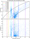 |
Fig. 1 Eccentricities (upper figure) and inclinations (bottom figure) of TNOs. The data are from the IAU Minor Planet Center database2. The dashed line and the dash-dotted line represent respectively q = 30 and q = 40 au perihelion distances. Vertical solid coloured lines indicate the main mean-motion resonances with Neptune. |
Scattered disc objects (SDOs)
These are the objects found in the scattered disc, which extends from 30 au to roughly 1000 au and interacts with Neptune by close encounters. The SDOs have perihelion distances in between 30 au and roughly 40 au and are mainly grey (or neutral) in colour (Sheppard 2010).
Detached objects
These have slightly larger perihelion distances than the SDOs and are no longer affected by close encounters with Neptune.
The first hypothesis for the very peculiar structure of the Kuiper belt was proposed by Malhotra (1993, 1995) who predicted the existence of objects in external mean-motion resonances with Neptune. In the model, these objects are trapped via adiabatic resonance sweeping during a phase of outward planetesimal-driven migration of the ice giant (Fernandez & Ip 1984). Indeed, resonance capture can occur when the orbital frequency of a planetesimal and/or a planet changes gradually and the resonance ‘sweeps’ across the orbit of the planetesimal. Resonance sweeping may result in the capture of the planetesimal in the resonance (if the migration direction is convergent and sufficiently slow), or in the excitation of the planetesimal to higher eccentricity without capture taking place (when the migration is divergent; Henrard & Lemaitre 1983). Since these latter publications, a myriad of studies have explored how the outward migration of Neptune can shape the trans-Neptunian region (Chiang et al. 2003; Gomes 2003; Hahn & Malhotra 2005; Levison et al. 2008; Nesvorný 2015a,b; Nesvorný & Vokrouhlický 2016). The accepted paradigm for HCs is that they formed inside 30 au and were implanted into the CKB region because of the outward migration of Neptune. Cold classicals are thought to be formed in situ, at >40 au, and to not have been significantly disturbed by the migration of Neptune, explaining the high rate of wide binaries in the population. Recent models seem to prefer a Neptune migration that was slow, long-range, and grainy (Nesvorný 2015a,b; Nesvorný & Vokrouhlický 2016). Nevertheless, the rich structure of the Kuiper belt is not easily reproducible. The main issues can be grouped into three topics: the colour problem, the inclination problem, and the resonant population problem.
The colour problem
Cold classicals have their own red colour (often referred to as very red or ultra-red in the literature) that is distinct from that of the dynamically excited population (HCs, resonant KBOs, and SDOs with i > 5°), whose members show a broad range of colours (Pike et al. 2017). Also, the overall colour distribution of dynamically excited TNOs is found to be bimodal and can be divided into a grey (or neutral) class and a red class. Red dynamically excited objects have lower inclinations (5° < i < 20°) and grey ones have a much wider inclination range. The different orbital distributions of the grey and red dynamically excited TNOs provide strong evidence that their colours are due to different formation locations in a disc of planetesimals with a compositional gradient (Marsset et al. 2019). This is potentially in agreement with the planetesimal-driven migration of Neptune because the higher inclinations of the grey (or neutral) dynamically excited TNOs imply that they have experienced more interaction with Neptune than the red ones (Gomes 2003), suggesting a grey–red–(CC)red composition of the primordial planetesimal disc. On the other hand, Fraser et al. (2017) reported the detection of a population of neutral-coloured, tenuously bound binaries residing among the CCs. These latter authors suggested that these binaries may be contaminants originating from about ≈38 au that survived being pushed out into the cold classicals during the early phases of Neptune’s migration. Schwamb et al. (2019), based on optical and near-infrared (NIR) colours of 35 TNOs and on the presence of neutral wide binaries in the CCs, formed the hypothesis of a protoplanetesimal disc with red–grey–(CC)red composition, with the excited red class closer to the Sun, the grey class (or neutral) in between ≈33 and ≈40 au, and the red CCs beyond 40 au, in contrast with Marsset et al. (2019). Hence, the colouring of the TNOs has a layer of complexity that remains to be disentangled.
The inclination problem
A long-standing problem of the different migration models of Neptune is that all of them produce, to a greater or less extent, a narrower inclination distribution of Plutinos and HCs compared to observations (Brown 2001; Gomes 2003; Nesvorný 2015a). The inclinations may have been excited prior to Neptune’s migration, but no such early excitation process has been identified so far (Chiang et al. 2003). The inclinations are also not strongly correlated with the timescale of Neptune’s migration (see Nesvorný 2015a; Volk & Malhotra 2019). The lack of cold Plutinos is also very puzzling: classical models reproduce this feature by truncating the planetesimal disc at about 34 au and letting Neptune ‘jump’ during the late instability of the giant planets (Levison et al. 2008).
The resonant population problem
Finally, models with a smooth migration of Neptune predict excessively populated resonances compared to the CKB population, which is estimated to contain more mass than Plutinos (Gladman et al. 2012). Nesvorný & Vokrouhlický (2016) showed that a grainy migration of Neptune cannot resolve the overpopulation problem of the resonances compared to the HCs, but produces better results for the ratios between the population in resonances, that is, the ratios between 3:2, 2:1, and 5:2 (see Malhotra 2019, Fig. 3). The 5:2 resonance, in particular, is very hard to populate with current models; it is a third-order resonance located at about 55 au and is expected to be relatively weak compared to the first-order resonances 2:1 and 3:2, but its population is probably comparable with Plutinos (Gladman et al. 2012; Volk et al. 2016). The concentration of their eccentricity near 0.4 was explained by Malhotra et al. (2018) as being related to the resonant width maximum near this value of eccentricity. Nevertheless, how a large number of objects ended up trapped in the 5:2 resonance is still an open question. Indeed, adiabatic resonance capture from an initially cold planetesimal disc is inconsistent with a very populated 5:2 resonance and its inclination distribution (Chiang et al. 2003). However, the resonance sweeping scenario of Malhotra (1993, 1995) could yield capture efficiencies in the 5:2 resonance approaching those of the 2:1 resonance if Neptune migrated smoothly into a prestirred planetesimal disc (Chiang et al. 2003; Hahn & Malhotra 2005). The alternative is the direct gravitational scattering, but this mechanism leads to large libration amplitudes (exceeding 160°) for the resonantKBOs, in contrast to observations.
Planet formation models have changed drastically since the discovery of the first (after Pluto and Charon) trans-Neptunian object in 1993 (Jewitt & Luu 1993). The main new idea is that the cores of the giant planets grow quickly according to the core accretion model (Pollack et al. 1996) boosted by pebble accretion (Johansen & Lacerda 2010; Ormel & Klahr 2010; Lambrechts & Johansen 2012; Ida et al. 2016; Johansen & Lambrechts 2017) and migrate inwards because of interactions with the gaseous disc (Ward 1997; Lin & Papaloizou 1986), following growth tracks similar to those shown in Bitsch et al. (2015). According to these models, the cores of giant planets form further away in the outer Solar System with respectto their current location and then migrate inwards while growing. Recently, Pirani et al. (2019a,b) showed thatthe inward migration of the giant planets could also have affected our Solar System. Indeed, the model can explain the Trojan asymmetry very easily: it arises because Jupiter was growing and migrating at the same time during the gaseous phase of the protoplanetary disc. These latter authors also showed that, in order to have an asymmetry comparable with the observed one, Jupiter must have migrated at least a few astronomical units (au). Also, based on compositional arguments, it has been suggested that Jupiter formed in the outer Solar System. Indeed, in Jupiter’s atmosphere, elements like C, N, S, P, Ar, Kr, and Xe are enriched with respect to solar values by approximately a factor of three. If Jupiter accreted around its current location, only some of those elements would have been in the solid phase in the solar nebula, whereas others (Ar and the main carrier of N, N2) would have still been volatile and would not have been accreted onto the core. Öberg & Wordsworth (2019) proposed the idea that Jupiter’s core formed beyond ≈30 au, where nitrogen and various noble gases were frozen and could be accreted by the core. Then, during envelope accretion and planetesimal bombardment, some of the core mixed with the envelope, causing the observed enrichment pattern.
If the large-scale migration of the giant planets happened in our Solar System, it could also have shaped the trans-Neptunian region, which is the scenario that we explore in the present paper. The paper is organised as follows: in Sect. 2 we describe the N-body code, and how we built the growth tracks and the different scenarios we tested in our simulations. In Sect. 3 we present our results and analyse the different features of the Kuiper belt obtained with every scenario. Finally, in Sect. 4 we summarise our results and discuss their implications.
2 Methods
In this study, we used a simplified version of the growth tracks of giant planets shown in Bitsch et al. (2015), that is, we followed the prescriptions presented in Johansen & Lambrechts (2017). We implemented the growth tracks into an N-body code and simulated the evolution of the Solar System over billions of years. We are interested in identifying features of the trans-Neptunuan region that are linked to the early inward migration of the giant planets. For this reason, we also need to mimic the subsequent planetesimal-driven migration of the ice giants and analyse how the shape of the Kuiper belt changes in response. We focus on the population of the MMRs with Neptune, the inclinations of the TNOs, and the formation location of the planetesimals that end up in the different populations of the trans-Neptunian region.
2.1 N-body code
In our simulations, we used a parallelised version of the MERCURY N-body code (Chambers 1999) and selected its hybrid symplectic integrator, which is faster than conventional N-body algorithms by about one order of magnitude (Wisdom & Holman 1991) and is particularly suitable for our simulations that involve timescales of the order of billions of years. We used a time-step that is 1/20 of the orbital period of the inner planet involved in the simulation (Duncan et al. 1998). We modified the code so that the giant planets grow and migrate according to the growth tracks generated following the recipes in Johansen & Lambrechts (2017), as is explained in Sect. 2.4.1.
In the MERCURY N-body code, planets are treated as massive bodies, and so they perturb and interact with all the other bodies during the integration. The other particles, called small bodies, are perturbed by the massive bodies but cannot affect each other. As we set them as ‘massless’, they also cannot perturb the massive bodies. We refer to these particles in the text as massless particles or small bodies. In our simulations, we used these massless particles to populate the planetesimal disc in which giant planets grow and migrate. Our version of the code also includes aerodynamic gas drag effects and tidal gas drag effects to mimic the presence of the gas in the protoplanetary disc, as in Pirani et al. (2019a). The growing protoplanets are affected by the tidal gas drag and the massless particles are affected by the aerodynamic gas drag from t = 0 Myr until the gaseous protoplanetary disc photoevaporates at t = 3 Myr according to typical disc lifetimes (Mamajek 2009; Williams & Cieza 2011). As small bodies are set to be massless during the integrations, we assign them a radius rp = 50 km (Johansen et al. 2014)and a density ρp = 1.0 g cm−3 when computing the effect of the aerodynamic gas drag.
In the MERCURY N-body, migration and gas drag forces have been added directly at the end of each half time-step as a series of symplectic steps to the integrator to account for the evolution of the objects. We switch to asteroidal coordinates, apply the symplectic steps, and switch back to Cartesian coordinates.
2.2 Planetesimal disc properties
We always start with a cold planetesimal disc with random eccentricities in the interval [0, 0.01], random inclinations in the interval [0°, 0.01°], and random semimajor axes in each Δa = 0.5 au annular region. We populate annular regions of width Δa = 0.5 au with 1000 massless particles each. The same number of particles in each annular region means a surface density proportional to r−1. The outer edge of the planetesimal disc is at 47 au. The inner edge is at 22 au. The small particles are colour-coded in the following way, as shown in Fig. 2:
-
Grey for particles initially orbiting inside 38 au.
-
Orange for particles starting in between 38 au and 41 au.
-
Red for particles starting beyond 41 au.
We decided to colour-code them in this way to mimic the grey–red–(CC)red composition of the primordial planetesimal disc suggested inMarsset et al. (2019). In this case, we use the orange colour to represent the red colour of the dynamically excited population of the KB and the red colour to represent the ultra-red colour of the CCs. The edge between the grey colour and the orange colour has been chosen so that the final SDOs of the different scenarios are predominantly grey. The edge between orange and red colours has been chosen to be 41 au because CCs are supposed to form roughly beyond this limit.
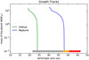 |
Fig. 2 Growth tracks of Neptune (blue curve) and Uranus (green curve) in our nominal model. The starting colour-coded planetesimal disc is shown at the bottom of the plot. |
2.3 No migration
As a starting point, we decided to explore the structure of the Kuiper belt region under the influence of the four giant planets in the current configuration. We used the starting parameters of Jupiter, Saturn, Neptune, and Uranus included in the MERCURY N-body code package. We populated the planetesimal disc from 22 to 47 au with massless particles: 1000 small bodies every annular region of width Δa = 0.5 au, for a total of 50 000 massless particles. We integrated the simulations for 4.5 Gyr, analysed which structures form in the trans-Neptunian region, and compared them with the ones produced in the alternative scenarios. We did not include any gas effect in this particular simulation because planets start as fully formed and in their current position. Simulations are set in the post-protoplanetary disc phase.
2.4 How Neptune can shape the Kuiper belt
As a second step, we decided to explore how Neptune, its formation location, and its migration could affect the contamination and excitation of the trans-Neptunian region. In these experiments we included only Neptune and Uranus for two main reasons: (1) the two ice giants are the main sources of influence to sculpt the Kuiper belt region and (2) the strong resonance shifting of the massive gas giants Jupiter and Saturn could easily destabilise the ice giant migration, requiring accurate fine tuning that would not necessarily add more information useful to this section of the modelling. The full system of the giant planets is added and explored in Sect. 2.5.
2.4.1 Inward migration
We first tested only inward migration of the ice giants. In order to generate the ‘growth tracks’ for Neptune and Uranus that we implement in our simulations, we used the recipes in Johansen & Lambrechts (2017). The disc parameters for our model are: fg = 0.2, fp = 0.4, fpla = 0.2, H∕r = 0.05, Hp /H = 0.1, Δv = 30 m s−1, and St = 0.1, where fg, fp, and fpla are parameterisations of the column densities (of the gas, pebbles, and planetesimals, respectively) relative to the standard profiles, H∕r is the disc aspect ratio, Hp ∕H is the particle midplane layer thickness ratio, Δv is the sub-Keplerian speed of the gas slowed down by the radial pressure support, and St is the Stokes number of the pebbles.
Figure 2 shows the growth tracks of the ice giants in the nominal model. The initial mass of the seeds is 10−2 M⊕ and they grow until they reach their current masses. The migration starts slightly after 2 Myr and stops when the gas dissipates at 3 Myr. In the nominal model, Neptune’s seed starts at 38 au and Uranus’ seed starts at 24 au, but we also tested different starting positions forthe ice giants by modifying the migration rate by a factor of greater than one (starting positions of the ice giants further away from the Sun, i.e. 39 and 40 au) or smaller than one (starting position of the ice giants closer to the Sun, i.e. 37, 36, 35, 33 au). After the disc phase, the ice giant eccentricities and inclinations are artificially increased to reach roughly the current values following a similar exponential to that of Eq. (1) with an e-folding time of τ = 5 Kyr. We analyse the different inward migrations of the ice giant planets and the signature that they would leave on the Kuiper belt.
2.4.2 Adding the planetesimal-driven migration
In a second test with only Uranus and Neptune, we included a planetesimal-driven migration (Malhotra 1993, 1995) right after the inward migration described in Sect. 2.4.1.
In order to add the planetesimal-driven migration, we followed the approach adopted in Minton & Malhotra (2009) and, just after the disc dispersal (t = 3 Myr), we let Uranus and Neptune migrate following the exponential law:
![Mathematical equation: \begin{equation*}a(t)\,{=}\,a_0+\Delta a[1-\textrm{exp}(-t/\tau)] ,\end{equation*}](/articles/aa/full_html/2021/06/aa37465-20/aa37465-20-eq1.png) (1)
(1)
where a0 is the initial semimajor axis and Δa is the final displacement. We also tested a delayed outward migration that starts at 13 Myr instead of 3 Myr because the exact moment at which outward migration should start has not yet been established and we wanted to test the possible effects of a delay; nevertheless, we did not find any significant difference in the simulations. We produced growth tracks for Neptune and Uranus where they end their inward migration in an inner orbit compared to the current ones. The final displacement for the subsequent instability was set in order for the ice giants to reach roughly their current semimajor axis, depending on the final position after the inward migration. The parameter τ is the migration e-folding time. We set τ = 10 Myr (Nesvorný 2015a).
We tested Neptune starting at 39, 37, and 35 au and an inward migration as deep as 21, 24, and 27 au for each different starting position. We obtained the different growth tracks by modifying the migration rate of the planets. Uranus growth tracks are scaled accordingly.
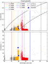 |
Fig. 3 Osculating eccentricities (top plots) and inclinations (bottom plots) of the trans-Neptunian region after 4.5 Gyr of integration. In this simulation the giant planets do not migrate and they are set with their current orbital parameters. Blue stars show particles that end up trapped as true resonant in 3:2, 5:3, 2:1, and 5:2 MMRs. The other particles in proximity to the MMRs are linked to the phenomenon of resonance sticking, that is they are only temporarily trapped in these MMRs and are therefore excluded from the true resonant objects group. |
2.5 Including all the giant planets
We repeated some of the migration simulations, this time including Jupiter and Saturn. We tested inward migration followed by the planetesimal-driven migration phase. Jupiter, Saturn, and Uranus seeds start at about 18, 21, 25 au, respectively, and reach their current semimajor axis after inward and outward migration. For the growth tracks of Neptune, we instead simulated two different cases: inward migration from (1) 38 to 21 au and from (2) 39 to 18 au, followed by outward migration to its current orbit.
3 Results
3.1 Fixed planets
In this simulation, Jupiter, Saturn, Neptune, and Uranus are fixed in their current locations and we let the system evolve for 4.5 Gyr to check the long-term effects on the Kuiper belt. In this case, as the planets start as fully formed and in their current configuration, we do not take into account any gas effects on planets or small bodies.
Results are shown in Fig. 3. As we can see, when the planets do not migrate at all, only sporadic true resonant objects are found. This is not surprising because capture by resonance sweeping requires convergent migration. Blue star symbols show the few particles that are trapped long term in the 3:2, 5:3, 2:1, and 5:2 MMRs with Neptune. We only included particles whose resonant angles2 show a long-term libration, meaning that they undergo bounded oscillations from 3 Myr to the end of the simulations (4.5 Gyr).
We notice that only two of them are really resonant; the other particles in the proximity of a MMR are linked to the phenomenon of resonance sticking (see Fig. 4 for some examples), defined as temporary resonance trapping (single or multiple) during the dynamical lifetime of the object that can also last for billions of years (Duncan & Levison 1997; Gladman et al. 2002; Lykawka & Mukai 2007). When analysing the resonant arguments of the objects labelled as ‘true resonant’, we notice that these two objects start directly in a MMR. As is expected, no object is trapped in MMR without convergent migration. The depletion inside 33 au is likely the classical chaotic zone of overlap of first-order MMRs. The plot also shows a gap in between roughly 40 and 42 au, which is due to the ν8 secular resonance with Neptune. Less particles ended up as HCs and some resonances, like the 2:1 and the 5:2, do not show a population of resonance sticking objects, in contrast to the 3:2 and the 5:3 resonances for the simple fact that there are noplanetesimals starting close to those resonance locations. The trans-Neptunian region also presents a scattered disc and few detached objects. We notice that the eccentricities of resonance sticking objects never become large enough for their perihelion distance to be closer to the Sun than Neptune, as is otherwise common in the observed resonant KB populations. Inclinations are also lower than those suggested by observations. In terms of the colour-code of the particles, the KB preserves its initial composition gradient with little or no mixing in between thedifferent populations. Only the SDOs present a mix of all three colours. Finally, we also observe that there is a leftover planetesimal disc with low eccentricities and low inclinations in between roughly 36 and 39 au. Even if it is not empty in the current architecture of the Solar System (see Fig. 1), this particular region is never sufficiently disturbed to get depleted during the simulations and ends up with too much mass.
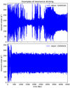 |
Fig. 4 Example of resonance sticking objects in our simulations. Here ϕ is the resonant angle. Objects in a MMR have values of ϕ that librate around a central value. In these examples, however, objects are only temporary trapped once or multiple times during the integration time. Some of these objects can show a very long-term sticking to the resonance, as shown in the bottom plot. |
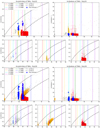 |
Fig. 5 Osculating eccentricities (left plots) and inclinations (right plots) of the trans-Neptunian region after 4.5 Gyr of integration. Neptune undergoes disc migration from 35 au (top plots) and 39 au (bottom plots) and reaches its current semimajor axis at about 30 au. Rows containing three plots highlight the separate coloured components. Blue stars and dots indicate true resonant objects. Compared to the ‘fixed planets’ case, the disc in between 34 and 39 au has been depleted by Neptune’s inward migration. If Neptune starts very close to the CKB region, some of the orange and grey planetesimals end up forming a low-i and moderate-e clump that overlaps in part with the CCs. |
3.2 How Neptune can shape the Kuiper belt
3.2.1 Inward migration
In this set of simulations, we consider only the inward migration of Neptune and Uranus during the gas-phase of the protoplanetary disc. After the disc phase, eccentricities and inclinations of the ice giants are artificially increased to reach roughly the current values as explained in Sect. 2.4.1. We tested different starting positions for Neptune’s seed and Uranus is scaled accordingly. Because we consider just the two ice giants, the positions of the secular resonances and their relative gaps may be displaced compared to the actual Solar System and their features are ignored in the analysis. We simply kept track of them.
We analysed the results for Neptune starting at 35 and 39 au and ending its migration in its current position. The other starting positions led to similar results and therefore are not shown here. Snapshots were taken after 4.5 Gyr of evolution and are shown in Fig. 5. We first studied the objects close to the resonant locations. We expected to find resonance sticking objects and maybe some true resonant objects that happened to start the simulation directly in the MMRs as in the ‘fixed planets’ case, because the migration is divergent and objects should not be trapped in external MMRs. However, the results are surprisingly different in this inward migration case. We computed the resonant angles for the objects close to the resonant locations and only labelled as true resonant those that have the resonant angle bounded from the dispersal of the disc (3 Myr) onwards until the end of the simulation (4.5 Gyr). We found 31 true resonant objects (22 in the 3:2 MMR and 9 in the 5:3 MMR) in the simulation where Neptune starts at 35 au and 260 true resonant objects (71 in the 3:2 MMR and 189 in the 5:3 MMR) in the simulation where Neptune starts at 39 au. None of them happened to start in a resonance from the beginning.
We analysed the semimajor axis, resonant angle, eccentricity, and inclination of these objects and Neptune and we show an example of that in Fig. 6. As we can see, these objects are disturbed by the inward migration of Neptune and are scattered bythe planet. What happens next is that they cross or stick to an external MMR when Neptune is increasing its eccentricity. Because of this, the resonance width increases and the object sinks into the resonance. The variety of the libration angle amplitudes of these objects also suggests that this is not a case of resonance sticking, but is a new trapping mechanism: scattering plus resonance sinking. We repeated the same simulation without artificially increasing the eccentricity or the inclination of Neptune at the end of the disc phase (3 Myr). We found very similar results to the previous case: at the end of the inward migration, Neptune finds itself close to the 2:1 mutual MMR with Uranus, and its eccentricity (which during the disc phase is of the order of 10−4) increases anyway and starts to oscillate in between values of roughly 0.001 and 0.01 in the ‘dance’ with Uranus.
Analysing the other features present in Fig. 5, we notice that none of the eccentricities of the true resonant objects become large enough that their perihelion distance is closer to the Sun than Neptune. Resonances 2:1 and 5:2 are empty because there is less chance for the resonance sinking mechanism to work where planetesimals are more dispersed. The scattered disc is very underpopulated and some detached objects are also present. The 3:2 resonance is a mix of grey and orange particles. Another very interesting result is that in cases where Neptune starts very close to the CC region, such as 38, 39, and 40 au, grey and orange particles are pushed into the CC region forming a population with low inclination and moderate eccentricity that overlaps with the CCs at about 42 au. The disc in between 34 and 39 au that survived in the ‘fixed planets’ case is much less populated in the inward migration cases because Neptune depletes the region while migrating inwards. There are some other differences in this region depending on where Neptune forms. If Neptune starts at 39 au, the ice giant scatters and excites many more grey objects (the ones inside 38 au). This leads to the possibility for them to reach the resonant locations and stick to them or sink in them. The majority of the survivors stick to the resonances or are truly trapped. In the case where Neptune forms at 35 au, objects are less disturbed by its formation and migration and have less chance to stick to distant resonances or to stick to nearby resonances with higher eccentricity. The gap in between 40 and 42 au is due to the secular resonance with Uranus and not Neptune (as in the current architecture of the Solar System), because we did not include all the giant planets in this particular set of simulations. Nevertheless, this is not relevant to the scope of this section, which is not to reproduce the correct structure of the KBO region, but to investigate how the initial position of Neptune can contaminate the CKBO region.
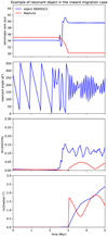 |
Fig. 6 Semimajor axis, resonant angle, eccentricity, and inclination of an object in true resonance with Neptune, from top to bottom, respectively. The red line refers to Neptune’s parameters, the blue line refers to the parameters of the true resonant object. |
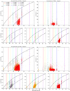 |
Fig. 7 Osculating eccentricities and inclinations of the trans-Neptunian region after 4.5 Gyr of integration. Neptune undergoes disc migration from 39 to 21 au (top plot) and 27 au (bottom plot) and then it reaches its current semimajor axis at about 30 au following Eq. (1). Rows containing three plots highlight the separate coloured components. There are some differences, mainly concerning the 3:2, 4:3, and 5:4 resonances; they are less populated if Neptune’s migration is as deep as 21 au. |
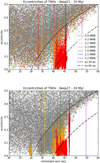 |
Fig. 8 Osculating eccentricities and inclinations of the trans-Neptunian region at 20 Myr. Neptune undergoes disc migration from 39 to 21 au and 27 au, and at 20 Myr it almost reaches its final position at about 30 au following Eq. (1). We notice that in the deep21 case, the degree of excitation of the belt is larger and, for example, the red objects that reach higher eccentricity are scattered when they become Neptune’s crossers. In the deep27 case, red objects do not reach enough eccentricity to be scattered around. Resonances (and Neptune’s position) are slightly shifted even if snapshots are taken at the same time because the displacement of the outward migration is different in the two cases and therefore so is the rate of outward migration. |
Percentage of the outer planetesimal disc left after the inward migration of Neptune.
3.2.2 Mass left in the planetesimal disc after the large-scale inward migration of Neptune
In the following section, we analyse a scenario where Neptune migrates first inward during the gas disc phase and then outward mimicking a planetesimal-driven migration because of the presence of the leftover external belt of planetesimals. In order for the planetesimal-driven migration to work, the planetesimal disc outside the orbit of Neptune has to survive the inward migration of Neptune. Estimates of the mass of the primordial disc of planetesimals outside Neptune’s orbit prior to the planetesimal-driven migration are of 10− 30 M⊕ (Nesvorný & Morbidelli 2012). Table 1 summarises our results, which show that the disc survives the early inward migration of Neptune (and Uranus) and preserves most of the mass. The surviving disc is in the range of 64.9–33.1% of the primordial one, depending on the different simulations. This means that the inward and outward migration would work for most of the starting mass range proposed for the leftover disc in which the planetesimal-driven migration of Neptune takes place.
As the particles are massless, for our mass computation, we counted the number of particles left in the disc versus the initial number in the same range of semimajor axis. The inner edge of the disc considered is the deepest semimajor axis reached with the early inward migration (18, 21, 24 and 27 au in the different simulations) when the outer edge is 30 au. Computations are done at 3 Myr, immediately after the inward migration has ceased. The following percentages take into account only the planetesimals originally formed inside 30 au, because that is supposed to be the outer edge of the massive leftover planetesimal disc. The contribution of planetesimals formed originally beyond 30 au and ending interior to it, before the outward migration, is considered negligible, because beyond ~30 au the number density of the planetesimals per au is at least two orders of magnitude smaller than interior to this limit, so that Neptune ceases its outward migration.
3.2.3 Adding the planetesimal-driven migration
In this set of simulations, we consider the inward migration of Neptune and Uranus in the disc followed by an outward migration to their current orbits. Figure 7 shows the eccentricities and the inclinations of objects in the trans-Neptunian region in the case where the Neptune seed starts at 39 au and undergoes inward migration to a depth of 21 au (top plots) and 27 au (bottom plots) followed by planetesimal-driven migration to its current orbit. Other cases with different starting positions of the ice giants led to similar results and so we do not show them. The snapshots were taken after 4.5 Gyr of evolution. As we can see, the MMRs with Neptune are populated, including the 2:1 resonance, in contrast with the previous cases. Nevertheless, resonance 5:2 is almost empty compared to the 3:2 and 2:1 resonances. A scattered disc and few detached objects are present. The HC region is still underpopulated compared to the CCs. The bodies in the 2:1 resonance have lower inclinations compared to those in the 3:2 resonance, as is also the case for the observations, but the overall inclination distributions of the MMRs are narrower than those suggested by observations. The Neptune crossers in the resonances are present in all combinations of starting and final positions tested, as expected, and this looks like a characteristic that belongs only to the outward migration of Neptune, in the sense that inward migration does not seem to be able to capture resonant objects that are also Neptune crossers. The gap in between 40 and 42 au is present (due to a secular resonance with Uranus, in this particular case with just two planets) and the planetesimal disc interior to 39 au has been depleted by the passage of Neptune in the inward migration phase.
As noticed also in the previous case, where there was only inward migration involved, grey and orange particles overlap with the red ones in the CC region. This is due to Neptune starting at 39 au, which is very close to the CC region. Nevertheless, when Neptune migrates as deep as 21 au, these interlopers are not pushed inside the CC region, because Neptune only becomes massive enough have this effect when it is already too far away from the CC region. The few objects in the 5:2 resonance are grey, and the SDOs are mostly grey, as in the observed populations. Also, the 3:2, 4:3, and 5:4 resonances are predominantly grey, in contrast with observations that show that the 3:2 resonance spans the full range of KBO colours. The 2:1 resonance is a mix of all three colours.
There is a trend of increasing depletion in the KB in simulations deep27, deep24, deep21, and deep18 (deep24 and deep18 not displayed in this paper). As shown in Fig. 8, this is due to the fact that the deeper the inward migration, the more the MMRs will cross the CKB region in the outward migration phase, leading to excitation and depletion (because of the close encounters with Neptune) of the objects that do not have the appropriate e and i to be trapped via resonance sweeping in resonances that widen only for a narrow parameter space. Therefore, the deeper the inward migration (or the more long-range the planetesimal-driven migration), the less populated are the main resonances, because there are less planetesimals available for capture. In the case where Neptune migrates as deep as 21 au, resonances 5:4 and 4:3 are almost empty compared to when it migrates deep to 27 au.
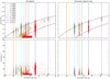 |
Fig. 9 Osculating eccentricities (top plots) and inclinations (bottom plots) of the trans-Neptunian region after 4.5 Gyr of evolution inthe case where Neptune starts from 38 au and migrates inwards to 21 au. All four giant planets undergo inward migration in the disc plus outward migration to their current orbits. In the left plots, only true resonant particles in the 3:2, 5:3, 7:4, 2:1, and 5:2 MMRs are displayed. Other resonances have not been checked. We notice that the 5:2 resonance is populated in this case, even if not as much as the other main MMRs. The plots also show inclination–colour and eccentricity–colour correlations for the particles. |
3.3 Including all the giant planets
In the last set of simulations, we included all the giant planets: Jupiter, Saturn, Uranus, and Neptune and we tested the inward–outward migration of the giant planets. Figure 9 shows snapshots at t = 4.5 Gyr of the simulations where Neptune starts at 38 au and migrates inwards to 21 au and then outwards to its current location. The outward migration of Neptune in this particular simulation starts 10 Myr after the disc dissipates, i.e. at 13 Myr. The results do not differ if we start the outward migration at 3 Myr.
Figure 9 reveals the presence of resonant KBOs that cross Neptune’s orbit, as expected. The scattered disc is well defined and detached objects are present. Many resonances are populated, many more than the previous cases analysed. The 5:2 resonance is underpopulated and the few objects in the resonance are mainly grey-orange.The HC region is more populated than the previous cases and the reason for this is the presence of Jupiter thatscatters objects outwards as shown in Fig. 10 when we compare the snapshot taken at 5 Myr of this simulation with the similar simulation deep21 (from 39 au), where only Neptune and Uranus are present. There is no significant difference at 3 Myr when the disc dissipates; however the two simulations diverge during the outward migration because of the enormous scattering efficiency of Jupiter. The overall i-distribution is nevertheless still narrower than seen in observations. The 3:2 resonance is mainly grey. The 2:1 resonance is mostly composed of red particles. The resonances in between are a mix of all three colours. As expected, there is a correlation between eccentricity and colour for the resonant objects. There is also a correlation between colours and inclinations of non-resonant objects, with the grey particles having the broadest inclination distribution, followed by the orange ones, and the red particles having the narrowest inclination distribution. This correlation between inclination and colour seems to be present also for other populations of the KB. Grey objects are the most excited by the migration of the giant planets and show higher inclinations than orange and red ones. Below roughly 15°, grey and orange planetesimals appear well mixed.
In the case where Neptune undergoes inward migration from 39 to 18 au and then outward migration to its current location, results are shown in Fig. 11. These plots show very different results from the previous case where Neptune migrated only to 21 au. A large number of particles end up in the resonance 5:2, which is six times more populated than the 3:2 MMR and mostly composed of red particles. This is because the 5:2 resonance sweeps the region roughly in between 33 and 55 au before the other resonances, depleting the region in which the other main MMRs will eventually sweep. It is not possible to efficiently capture bodies in the 5:2 resonance from an unperturbed disc (see Chiang et al. 2003 or the recent review by Malhotra 2019) because of the shape of the resonance. As explained in Chiang et al. (2003), the capture probability only increases if the disc is prestirred. When Neptune migrates inwards to 21 au as in the previous scenario, the 5:2 resonance crosses a disc that is almost completely unperturbed, because Neptune forms at 39 au and the stirred region is very narrow. In this simulation, instead, the inward migration of Neptune is deeper and the 5:2 resonance goes as deep as 33 au, crossing the region already stirred by the formation of Neptune and the region of red objects (swept and excited by many other resonances), leading to a very efficient capture in the subsequent convergent migration. The CKB is depleted, but so are the resonant populations. Moreover, other weaker MMRs in between 2:1 and 5:2 are found to be populated. Resonance 3:2 is composed of mainly grey particles, as is the 2:1 resonance, in contrast with the previous simulation. The gap in between 40 and 42 au is now correctly due to a secular resonance with Neptune. The correlation between eccentricity and colour in the resonant object is not as clear as in the previous case.
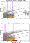 |
Fig. 10 Comparison between the simulation including all the giant planets and simulation deep21 (from 39 au), where only Neptune and Uranus are present. The snapshots were taken at 5 Myr, when the disc phase (and therefore the inward migration) has already ended and the planets are undergoing outward migration, as highlighted by the different locations of the MMRs. The simulations diverge during the outward migration because of the enormous scattering efficiency of Jupiter. |
4 Discussion and conclusions
In this study, we performed simulations of different scenarios that include inwards migration of the giant planets during the gas-disc phase and analysed how they shape the trans-Neptunian region. We started with the giant planets in fixed positions, and then considered inward migration of the ice giants, and we also added planetesimal-driven outward migration to their evolution. We concluded our investigation by performing inward migration for all four giant planets plus outward migration. We colour-coded our planetesimal disc in the following way: the grey particles are initially placed inside 38 au; the orange ones in between 38 and 41 au, and the red ones in between 41 and 47 au. Our main conclusions are as follows.
- (i)
Bodies can resonantly stick to the external MMRs in the KB in the absence of Neptune migration. In the case of inward migration, in addition to resonance sticking, objects can also end up truly trapped in the MMRs. Nevertheless, Neptune crossers in MMRs are a unique signature of the outward planetesimal-driven migration of Neptune, in the sense that only inward migration does not seem to be able to capture resonant objects that are also Neptune crossers.
- (ii)
Inward migration suggests an additional channel to populate the external MMRs with Neptune: scattered objects sticking temporarily to a MMR can sink deeper in the resonance when Neptune increases its eccentricity. Therefore, those objects become true resonant objects via the ‘resonance sinking’ mechanism which does not require convergent migration.
- (iii)
The 5:2 and 2:1 MMRs with Neptune do not end up populated with true resonant objects in the fixed planets scenario because capture by resonance sweeping requires convergent migration. When we consider only the inward migration of Neptune and Uranus and the new resonance trapping mechanism (resonance sinking), there is less chance of scattered objects being trapped because these two resonances do not cross the region initially populated by planetesimals. The scattered objects are then too dispersed beyond the edge of the planetesimal disc, and their chances of ending up in these resonances are minimised.
- (iv)
When we include all four giant planets, the inward migration of Jupiter stirs all the objects in the Solar System, including the trans-Neptunian ones. The result is that we ended up with a significant fraction of HCs compared to the cases where we included only Neptune and Uranus.
- (v)
The formation location of Neptune and its growth rate may influence the CKB region. Indeed, if Neptune becomes massive enough when it is still very close to the CKB region, it is able to push particles from the neighbouring region into it, creating a population of moderate-e and moderate-i particles that can overlap with CCs. This could be another possible way to push out neutral-coloured wide binaries – if they survive – into the CC region before the outward migration starts, when Neptune is not very massive yet and the gaseous protoplanetary disc is still in place.
- (vi)
The population of the resonance 5:2 depends on the depth of the inward migration. In this paper we analysed a Neptunestarting its outward migration from 21 au and from 18 au and the 5:2 resonance was scarcely populated in the former case and was six times more populated than the 3:2 resonance in the latter. This is because, in the latter case, the5:2 MMR resonance sweeps a wider region populated with excited planetesimals.
- (vii)
Grey objects are more excited by the migration of the giant planets and they end up with the highest inclinations among the colour-coded ones. Below roughly 15°, grey andorange planetesimals seem well mixed. This confirms the results of Gomes (2003) and is in agreement with the grey–red–(CC)red primordial planetesimal disc (Marsset et al. 2019).
- (viii)
Based on the simulations, we find the expected correlation between eccentricity and colour of resonant objects, which reflects the primordial composition of the disc.
- (ix)
Chiang et al. (2003) found that in order to trap objects in the 5:2 resonance, the primordial trans-Neptunian planetesimal disc must be prestirred. The deep inward migration of the giant planets seems to be the missing mechanism able to stir the trans-Neptunian region prior to the outward planetesimal-driven migration.
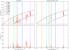 |
Fig. 11 Osculating eccentricities (top plots) and inclinations (bottom plots) of the trans-Neptunian region after 4.5 Gyr of evolution in the case where Neptune starts from 39 au and migrates inwards to 18 au, then migrates outwards to its current location. All the four giant planets undergo inward plus outward migration to their current orbits. In the right plots only resonant particles in the 3:2, 5:3, 7:4, 2:1 and 5:2 MMRs are displayed. We found that in this case the resonance 5:2 is six times more populated than the 3:2 MMR. Moreover, the CKB is depleted compared to the previous cases, but so are the resonant populations. |
Acknowledgements
We would like to thank the referee for the comments that helped us to improve our work. SP, AJ and AM are supported by the project grant ‘IMPACT’ from the Knut and Alice Wallenberg Foundation (grant 2014.0017). AJ was further supported by the Knut and Alice Wallenberg Foundation grants 2012.0150 and 2014.0048, the Swedish Research Council (grant 2018-04867) and the European Research Council (ERC Consolidator Grant 724 687- PLANETESYS). The computations are performed on resources provided by the Swedish Infrastructure for Computing (SNIC) at the LUNARC-Centre in Lund and partially funded by the Royal Physiographic Society of Lund through a grant.
References
- Bernstein, G. M., Trilling, D. E., Allen, R. L., et al. 2004, AJ, 128, 1364 [NASA ADS] [CrossRef] [Google Scholar]
- Bitsch, B., Lambrechts, M., & Johansen, A. 2015, A&A, 582, A112 [NASA ADS] [CrossRef] [EDP Sciences] [Google Scholar]
- Brown, M. E. 2001, AJ, 121, 2804 [Google Scholar]
- Chambers, J. E. 1999, MNRAS, 304, 793 [Google Scholar]
- Chiang, E. I., Jordan, A. B., Millis, R. L., et al. 2003, AJ, 126, 430 [NASA ADS] [CrossRef] [Google Scholar]
- Di Ruscio, A., Fienga, A., Durante, D., et al. 2020, A&A, 640, A7 [CrossRef] [EDP Sciences] [Google Scholar]
- Duncan, M. J., & Levison, H. F. 1997, Science, 276, 1670 [NASA ADS] [CrossRef] [PubMed] [Google Scholar]
- Duncan, M. J., Levison, H. F., & Lee, M. H. 1998, AJ, 116, 2067 [NASA ADS] [CrossRef] [EDP Sciences] [Google Scholar]
- Fernandez, J. A., & Ip, W.-H. 1984, Icarus, 58, 109 [NASA ADS] [CrossRef] [Google Scholar]
- Fraser, W. C., Brown, M. E., Morbidelli, A., Parker, A., & Batygin, K. 2014, ApJ, 782, 100 [NASA ADS] [CrossRef] [Google Scholar]
- Fraser, W. C., Bannister, M. T., Pike, R. E., et al. 2017, Nat. Astron., 1, 0088 [CrossRef] [Google Scholar]
- Gladman, B., Kavelaars, J. J., Petit, J.-M., et al. 2001, AJ, 122, 1051 [NASA ADS] [CrossRef] [Google Scholar]
- Gladman, B., Holman, M., Grav, T., et al. 2002, Icarus, 157, 269 [NASA ADS] [CrossRef] [Google Scholar]
- Gladman, B., Marsden, B. G., & Vanlaerhoven, C. 2008, Nomenclature in the Outer Solar System, eds. M. A. Barucci, H. Boehnhardt, D. P. Cruikshank, A. Morbidelli, & R. Dotson (Tucson: University of Arizona Press), 43 [Google Scholar]
- Gladman, B., Lawler, S. M., Petit, J. M., et al. 2012, AJ, 144, 23 [Google Scholar]
- Gomes, R. S. 2003, Icarus, 161, 404 [Google Scholar]
- Grundy, W. M., Noll, K. S., Nimmo, F., et al. 2011, Icarus, 213, 678 [NASA ADS] [CrossRef] [Google Scholar]
- Gulbis, A. A. S., Elliot, J. L., & Kane, J. F. 2006, Icarus, 183, 168 [NASA ADS] [CrossRef] [Google Scholar]
- Hahn, J. M., & Malhotra, R. 2005, AJ, 130, 2392 [NASA ADS] [CrossRef] [Google Scholar]
- Henrard, J., & Lemaitre, A. 1983, Celes. Mech., 30, 197 [Google Scholar]
- Ida, S., Guillot, T., & Morbidelli, A. 2016, A&A, 591, A72 [NASA ADS] [CrossRef] [EDP Sciences] [Google Scholar]
- Jewitt, D., & Luu, J. 1993, Nature, 362, 730 [NASA ADS] [CrossRef] [Google Scholar]
- Johansen, A., & Lacerda, P. 2010, MNRAS, 404, 475 [NASA ADS] [Google Scholar]
- Johansen, A., & Lambrechts, M. 2017, Ann. Rev. Earth Planet. Sci., 45, 359 [NASA ADS] [CrossRef] [Google Scholar]
- Johansen, A., Blum, J., Tanaka, H., et al. 2014, in Protostars and Planets VI, eds. H. Beuther, R. S. Klessen, C. P. Dullemond, & T. Henning (Tucson: University of Arizona Press), 547 [Google Scholar]
- Kavelaars, J. J., Jones, R. L., Gladman, B. J., et al. 2009, AJ, 137, 4917 [NASA ADS] [CrossRef] [Google Scholar]
- Lambrechts, M., & Johansen, A. 2012, A&A, 544, A32 [CrossRef] [EDP Sciences] [Google Scholar]
- Levison, H. F., Morbidelli, A., Van Laerhoven, C., Gomes, R., & Tsiganis, K. 2008, Icarus, 196, 258 [Google Scholar]
- Lin, D. N. C., & Papaloizou, J. 1986, ApJ, 309, 846 [NASA ADS] [CrossRef] [Google Scholar]
- Lykawka, P. S., & Mukai, T. 2007, Icarus, 192, 238 [CrossRef] [Google Scholar]
- Malhotra, R. 1993, Nature, 365, 819 [CrossRef] [Google Scholar]
- Malhotra, R. 1995, AJ, 110, 420 [NASA ADS] [CrossRef] [Google Scholar]
- Malhotra, R. 2019, Geosci. Lett., 6, 12 [CrossRef] [Google Scholar]
- Malhotra, R., Lan, L., Volk, K., & Wang, X. 2018, AJ, 156, 55 [CrossRef] [Google Scholar]
- Mamajek, E. E. 2009, AIP Conf. Ser., 1158, 3 [Google Scholar]
- Marsset, M., Fraser, W. C., Pike, R. E., et al. 2019, AJ, 157, 94 [CrossRef] [Google Scholar]
- Minton, D. A., & Malhotra, R. 2009, Nature, 457, 1109 [NASA ADS] [CrossRef] [PubMed] [Google Scholar]
- Nesvorný, D. 2015a, AJ, 150, 73 [NASA ADS] [CrossRef] [Google Scholar]
- Nesvorný, D. 2015b, AJ, 150, 68 [NASA ADS] [CrossRef] [Google Scholar]
- Nesvorný, D., & Morbidelli, A. 2012, AJ, 144, 117 [NASA ADS] [CrossRef] [Google Scholar]
- Nesvorný, D., & Vokrouhlický, D. 2016, ApJ, 825, 94 [NASA ADS] [CrossRef] [Google Scholar]
- Noll, K. S., Grundy, W. M., Chiang, E. I., Margot, J. L., & Kern, S. D. 2008, Binaries in the Kuiper Belt, eds. M. A. Barucci, H. Boehnhardt, D. P. Cruikshank, A. Morbidelli, & R. Dotson (Tucson: University of Arizona Press), 345 [Google Scholar]
- Öberg, K. I., & Wordsworth, R. 2019, AJ, 158, 194 [Google Scholar]
- Ormel, C. W., & Klahr, H. H. 2010, A&A, 520, A43 [NASA ADS] [CrossRef] [EDP Sciences] [Google Scholar]
- Parker, A. H., & Kavelaars, J. J. 2010, ApJ, 722, L204 [NASA ADS] [CrossRef] [Google Scholar]
- Petit, J. M., Kavelaars, J. J., Gladman, B. J., et al. 2011, AJ, 142, 131 [NASA ADS] [CrossRef] [Google Scholar]
- Pike, R. E., Fraser, W. C., Schwamb, M. E., et al. 2017, AJ, 154, 101 [NASA ADS] [CrossRef] [Google Scholar]
- Pirani, S., Johansen, A., Bitsch, B., Mustill, A. J., & Turrini, D. 2019a, A&A, 623, A169 [NASA ADS] [CrossRef] [EDP Sciences] [Google Scholar]
- Pirani, S., Johansen, A., & Mustill, A. J. 2019b, A&A, 631, A89 [CrossRef] [EDP Sciences] [Google Scholar]
- Pitjeva, E. V., & Pitjev, N. P. 2018, Celes. Mech. Dyn. Astron., 130, 57 [NASA ADS] [CrossRef] [Google Scholar]
- Pollack, J. B., Hubickyj, O., Bodenheimer, P., et al. 1996, Icarus, 124, 62 [NASA ADS] [CrossRef] [Google Scholar]
- Schwamb, M. E., Fraser, W. C., Bannister, M. T., et al. 2019, ApJS, 243, 12 [CrossRef] [Google Scholar]
- Sheppard, S. S. 2010, AJ, 139, 1394 [NASA ADS] [CrossRef] [PubMed] [Google Scholar]
- Volk, K., & Malhotra, R. 2019, AJ, 158, 64 [CrossRef] [Google Scholar]
- Volk, K., Murray-Clay, R., Gladman, B., et al. 2016, AJ, 152, 23 [NASA ADS] [CrossRef] [Google Scholar]
- Ward, W. R. 1997, Icarus, 126, 261 [Google Scholar]
- Williams, J. P., & Cieza, L. A. 2011, ARA&A, 49, 67 [NASA ADS] [CrossRef] [Google Scholar]
- Wisdom, J., & Holman, M. 1991, AJ, 102, 1528 [NASA ADS] [CrossRef] [Google Scholar]
It is worth mentioning that Fraser et al. (2014) estimate that the hot population is about 30 times more massive than the cold one. However, the definitions of hot and cold classes differ from the CC and HC classes. The cold objects are defined as having i < 5° and semimajor axis in the range of 38 au ≤a ≤ 48 au, while hot objects are within 30 au ≤R ≤ 150 au (a much larger region compared to the HCs one) with i > 5°.
In order to compute the resonant angle, we used the simplified formula ϕ = pλkbo − qλN − (p − q)ϖkbo, where λ and ϖ are the mean longitude and the longitude of perihelion, respectively. p and q are the small integers that relate the orbital periods of the two objects in resonance, p : q, with p > q > 0 for external resonances.
All Tables
Percentage of the outer planetesimal disc left after the inward migration of Neptune.
All Figures
|
Fig. 1 Eccentricities (upper figure) and inclinations (bottom figure) of TNOs. The data are from the IAU Minor Planet Center database2. The dashed line and the dash-dotted line represent respectively q = 30 and q = 40 au perihelion distances. Vertical solid coloured lines indicate the main mean-motion resonances with Neptune. |
| In the text | |
|
Fig. 2 Growth tracks of Neptune (blue curve) and Uranus (green curve) in our nominal model. The starting colour-coded planetesimal disc is shown at the bottom of the plot. |
| In the text | |
|
Fig. 3 Osculating eccentricities (top plots) and inclinations (bottom plots) of the trans-Neptunian region after 4.5 Gyr of integration. In this simulation the giant planets do not migrate and they are set with their current orbital parameters. Blue stars show particles that end up trapped as true resonant in 3:2, 5:3, 2:1, and 5:2 MMRs. The other particles in proximity to the MMRs are linked to the phenomenon of resonance sticking, that is they are only temporarily trapped in these MMRs and are therefore excluded from the true resonant objects group. |
| In the text | |
|
Fig. 4 Example of resonance sticking objects in our simulations. Here ϕ is the resonant angle. Objects in a MMR have values of ϕ that librate around a central value. In these examples, however, objects are only temporary trapped once or multiple times during the integration time. Some of these objects can show a very long-term sticking to the resonance, as shown in the bottom plot. |
| In the text | |
|
Fig. 5 Osculating eccentricities (left plots) and inclinations (right plots) of the trans-Neptunian region after 4.5 Gyr of integration. Neptune undergoes disc migration from 35 au (top plots) and 39 au (bottom plots) and reaches its current semimajor axis at about 30 au. Rows containing three plots highlight the separate coloured components. Blue stars and dots indicate true resonant objects. Compared to the ‘fixed planets’ case, the disc in between 34 and 39 au has been depleted by Neptune’s inward migration. If Neptune starts very close to the CKB region, some of the orange and grey planetesimals end up forming a low-i and moderate-e clump that overlaps in part with the CCs. |
| In the text | |
|
Fig. 6 Semimajor axis, resonant angle, eccentricity, and inclination of an object in true resonance with Neptune, from top to bottom, respectively. The red line refers to Neptune’s parameters, the blue line refers to the parameters of the true resonant object. |
| In the text | |
|
Fig. 7 Osculating eccentricities and inclinations of the trans-Neptunian region after 4.5 Gyr of integration. Neptune undergoes disc migration from 39 to 21 au (top plot) and 27 au (bottom plot) and then it reaches its current semimajor axis at about 30 au following Eq. (1). Rows containing three plots highlight the separate coloured components. There are some differences, mainly concerning the 3:2, 4:3, and 5:4 resonances; they are less populated if Neptune’s migration is as deep as 21 au. |
| In the text | |
|
Fig. 8 Osculating eccentricities and inclinations of the trans-Neptunian region at 20 Myr. Neptune undergoes disc migration from 39 to 21 au and 27 au, and at 20 Myr it almost reaches its final position at about 30 au following Eq. (1). We notice that in the deep21 case, the degree of excitation of the belt is larger and, for example, the red objects that reach higher eccentricity are scattered when they become Neptune’s crossers. In the deep27 case, red objects do not reach enough eccentricity to be scattered around. Resonances (and Neptune’s position) are slightly shifted even if snapshots are taken at the same time because the displacement of the outward migration is different in the two cases and therefore so is the rate of outward migration. |
| In the text | |
|
Fig. 9 Osculating eccentricities (top plots) and inclinations (bottom plots) of the trans-Neptunian region after 4.5 Gyr of evolution inthe case where Neptune starts from 38 au and migrates inwards to 21 au. All four giant planets undergo inward migration in the disc plus outward migration to their current orbits. In the left plots, only true resonant particles in the 3:2, 5:3, 7:4, 2:1, and 5:2 MMRs are displayed. Other resonances have not been checked. We notice that the 5:2 resonance is populated in this case, even if not as much as the other main MMRs. The plots also show inclination–colour and eccentricity–colour correlations for the particles. |
| In the text | |
|
Fig. 10 Comparison between the simulation including all the giant planets and simulation deep21 (from 39 au), where only Neptune and Uranus are present. The snapshots were taken at 5 Myr, when the disc phase (and therefore the inward migration) has already ended and the planets are undergoing outward migration, as highlighted by the different locations of the MMRs. The simulations diverge during the outward migration because of the enormous scattering efficiency of Jupiter. |
| In the text | |
|
Fig. 11 Osculating eccentricities (top plots) and inclinations (bottom plots) of the trans-Neptunian region after 4.5 Gyr of evolution in the case where Neptune starts from 39 au and migrates inwards to 18 au, then migrates outwards to its current location. All the four giant planets undergo inward plus outward migration to their current orbits. In the right plots only resonant particles in the 3:2, 5:3, 7:4, 2:1 and 5:2 MMRs are displayed. We found that in this case the resonance 5:2 is six times more populated than the 3:2 MMR. Moreover, the CKB is depleted compared to the previous cases, but so are the resonant populations. |
| In the text | |
Current usage metrics show cumulative count of Article Views (full-text article views including HTML views, PDF and ePub downloads, according to the available data) and Abstracts Views on Vision4Press platform.
Data correspond to usage on the plateform after 2015. The current usage metrics is available 48-96 hours after online publication and is updated daily on week days.
Initial download of the metrics may take a while.