© ESO 2021

1. Introduction

Magnetic flux cancellation is the process whereby two opposite polarities approach each other, interact via magnetic reconnection, and eventually submerge into the solar interior (e.g. Harvey 1985; Martin et al. 1985; Priest et al. 1987; van Ballegooijen & Martens 1989). In recent years, flux cancellation has been associated with a variety of solar phenomena and its importance has been re-examined. For example, observations above cancellation regions have revealed that flux cancellation is commonly associated with localised energy release events, such as Ellerman and IRIS bombs, UV and EUV bursts, and the corresponding reconnection-driven outflows and jets above such regions (e.g. Watanabe et al. 2011; Vissers et al. 2013; Peter et al. 2014; Rezaei & Beck 2015; Tian et al. 2016; Reid et al. 2016; Hong et al. 2017; van der Voort et al. 2017; Ulyanov et al. 2019; Huang et al. 2019; Chen et al. 2019; Ortiz et al. 2020; Park 2020). Another example is eruption-driven jets, where flux cancellation is often associated with the formation and triggering of erupting mini-filaments (e.g. Sterling et al. 2015, 2016; Panesar et al. 2016, 2019).

Aside from bursts and jets, observations have suggested that the cancellation of opposite polarities at the footpoints of coronal loops could be responsible for the brightening of coronal loops (Tiwari et al. 2014; Chitta et al. 2017, 2018; Huang et al. 2018; Şahin et al. 2019). Potentially, even spicules could be linked to flux cancellation (Sterling & Moore 2016; Samanta et al. 2019). Recent observations from the Sunrise balloon mission (Solanki et al. 2010, 2017), with a spatial resolution six times better than that of the Helioseismic Imager (HMI) on the Solar Dynamics Observatory (SDO), have shown that flux cancellation is occurring at rate that is an order of magnitude higher than previously thought (Smitha et al. 2017).

Inspired by these observations, Priest et al. (2018) proposed that nanoflares driven by flux cancellation could heat the solar chromosphere and corona. Their model was further developed with numerical simulations, demonstrating the validity of the theoretical model and showing that a variety of reconnection-driven jets with different properties can be formed by flux cancellation (Syntelis et al. 2019; Syntelis & Priest 2020).

This first presentation of this flux-cancellation model described the reconnection, examined above, which is driven by the convergence of two approaching polarities of equal flux in the presence of a horizontal ambient field. The analysis treated the current sheet as a two-dimensional object. In a new series of papers, we are further developing the model by treating the current sheet as an inherently three-dimensional structure and by extending the model to other geometries. As a first step, Priest & Syntelis (2021; herafter Paper I) derived the magnetic field strength in the vicinity of a three-dimensional toroidal current, taking its curvature into account. They also worked out the resulting three-dimensional correction to the model of Priest et al. (2018).

In the present work (Paper II), we take the next step in the development of the theory by examining more realistic magnetic configurations, where the two cancelling polarities have different fluxes. Thus, in this study, we examine the reconnection between two cancelling opposite polarities of unequal flux in the presence of a horizontal field. In Sect. 2, we present the theoretical model. In Sects. 3 and 4, we discuss our results and conclusions.

2. Theory of energy release at a reconnecting current sheet driven by the cancellation of unequal polarities

2.1. Magnetic configuration

Let us consider two sources of flux in the photospheric xy-plane. Source 1 has positive flux (F) and is situated at (d, 0), whereas source 2 is a parasitic polarity with negative flux (−F_p) with F_p ≤ F, and is situated at ( − d, 0). The local overlying magnetic field ($B_0\widehat{\mathbf{x}}$) is horizontal and is aligned with the two sources. The two sources approach one another, moving along the line that joins them at velocities that are slow enough (±v₀) so that the field passes through a series of equilibria.

The overall behaviour of the magnetic field during the approach of the sources is shown in Fig. 1, which depicts a vertical section through an axisymmetric configuration. It summarises schematically the slow-time evolution of the system through a series of equilibrium states. When the two sources, indicated by stars, are so far apart that they are not connected magnetically, their fluxes are bound by axisymmetric separatrix surfaces, shown as dashed lines that meet the x-axis at 3D null points N₁ and N₂ (Fig. 1a).

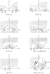Fig. 1. Overall behaviour of the magnetic field during the approach of two oppositely directed photospheric polarities (stars) of flux, −Fp and F, (where |Fp|< |F|) are separated by a distance, 2d, and situated in an overlying uniform horizontal magnetic field (B0). The magnetic field is axisymmetric, shown here in a vertical (y = 0) plane. Dashed curves show separatrix magnetic field lines and solid curves indicate other magnetic field lines. The separator is marked by an unfilled dot, and null points with solid dots. The field is shown for (a) d > dc1, when the two sources are far apart, (b) d = dc1, when the nulls coalesce at the photosphere (z = 0) and a separator first appears, (c) dc2 < d < dc1 (phase 1a), when the separator arches above the surface, (d) dc2 < d < dc1 (phase 1a), when the separator has moved to the left of the flux source −Fp, (e) d = dc2, when the separator falls back down to the photosphere and becomes a second-order null, (f) 0 < d < dc2 (phase 1b), when the null has bifurcated into two null points moving away from each other, and (g) d = 0, when the two sources have coalesced, leaving behind the remaining magnetic fragment of flux (F − Fp). Panel h: notation used to describe the reconnection process at a current sheet of length L.

As the sources approach one another, the nulls eventually coalesce to form a second-order null, which then becomes a separator (S) that rises above the photosphere (Fig. 1c). Reconnection is driven at S, which consists of an axisymmetric ring of null points and about which a separatrix current sheet forms (Fig. 1h). We note that a slight perturbation of the axisymmetric configuration would turn S into a separator having a magnetic field component along it and join two 3D nulls that lie in the photosphere. Eventually, the separator moves back down to the photosphere, where it becomes a null point that splits into two nulls (Fig. 1f) and which themselves eventually coalesce as the flux sources combine to leave behind a source of magnitude (F − F_p) (Fig. 1g). We now proceed to work out some of the details of this process.

The magnetic field above the photosphere (z > 0) is then given by:

$$\begin{array}{c}\hfill \mathit{B}=\frac{F}{2\pi }\frac{{\mathit{r}}_{\mathbf{1}}}{{r_1}^3}-\frac{F_p}{2\pi }\frac{{\mathit{r}}_{\mathbf{2}}}{{r_2}^3}+B_0\widehat{\mathbf{x}},\end{array}$$(1)

where

$$\begin{array}{c}\hfill {\mathit{r}}_{\mathbf{1}}=(x+d)\widehat{\mathbf{x}}+y\widehat{\mathbf{y}}+z\widehat{\mathbf{z}},{\mathit{r}}_{\mathbf{2}}=(x-d)\widehat{\mathbf{x}}+y\widehat{\mathbf{y}}+z\widehat{\mathbf{z}}\end{array}$$

are the position vectors of a point P(x, y, z) with respect to the two sources.

Magnetic fields are non-dimensionalised with respect to B₀, fluxes with respect to F and lengths with respect to the interaction distance (Longcope 1998):

$$\begin{array}{c}\hfill d_0={\left(\frac{F}{\pi B_0}\right)}^{1/2}.\end{array}$$(2)

The resulting dimensionless variables are $\overline{B}=B/B_0$, $\overline{d}=d/d_0$, $\overline{r}=r/d_0,$ and ${\overline{F}}_p=F_p/F,$ while Eq. (1) becomes:

$$\begin{array}{c}\hfill \overline{\mathit{B}}=\frac{{\overline{\mathit{r}}}_{\mathbf{1}}}{2{\overline{r}}_{\mathbf{1}}^3}-{\overline{F}}_p\frac{{\overline{\mathit{r}}}_{\mathbf{2}}}{2{\overline{r}}_{\mathbf{2}}^3}+\widehat{\mathbf{x}}.\end{array}$$(3)

From here onward, we omit the bars, so that all variables are dimensionless unless stated otherwise.

Due to the axial symmetry about the x-axis, we can set y = 0 to find the height of separator in the xz-plane, where B_x = B_z = 0, namely,

$$\begin{array}{c}\hfill \frac{x-d}{{r_1}^3}-F_p\frac{x+d}{{r_2}^3}+2=0,\frac{z}{{r_1}^3}-F_p\frac{z}{{r_2}^3}=0.\end{array}$$(4)

Solving these equations gives the coordinates (x_s, z_s) of the separator as

$$\begin{array}{c}\hfill x_s=\frac{1}{4d^{1/3}}({F_p}^{2/3}-1),z_s=\sqrt{d^{2/3}-{(\frac{{F_p}^{2/3}-1}{4d^{1/3}}-d)}^2}.\end{array}$$(5)

In Figs. 2a,b we plot x_s and z_s as functions of d for different values of F_p. As d decreases, the height of the separator goes from zero, to a maximum value, and then back to zero. The maximum z_s can found by setting the first derivative of the above expression for z_s to zero and is shown in Fig. 2 as green points. It occurs for

$$\begin{array}{c}\hfill d_{z_{s,\max }}={\left[\frac{1}{12}(F_p^{2/3}+1+2\sqrt{F_p^{4/3}-F_p^{2/3}+1})\right]}^{3/4}.\end{array}$$(6)

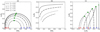Fig. 2. Position of the separator during Phase 1. (a) Height (zs) of the separator as a function of the half-separation (d) for different values of the minority flux (Fp). The coloured points mark the locations of the maximum zs (green) and the critical points where zs = 0 for d = dc1 (blue) and d = dc2 (red). (b) Horizontal position (xs) of the separator as a function of d. (c) Positions (xs, zs) of the separator in the y = 0 plane as d varies for different values of Fp.

Figure 2a reveals that for each value of F_p, there are two critical points where z_s = 0, so that the separator has become a null point at the photosphere. To find them, we set $z_s^2=0$ and solve for d, which gives

$$\begin{array}{c}\hfill \pm d^{1/3}=\frac{F_p^{2/3}-1}{4d^{1/3}}-d,\end{array}$$

where the conditions F_p < 1 and d > 0 rule out the positive solution, so that the above equation may be rewritten as a quadratic equation for d^2/3, namely,

$$\begin{array}{c}\hfill {\left(d^{2/3}\right)}^2-d^{2/3}-\frac{1}{4}(F_p^{2/3}-1)=0.\end{array}$$

This has two solutions:

$$\begin{array}{c}\hfill d_{c_1}={\left[\frac{1}{2}(1+F_p^{1/3})\right]}^{3/2}\mathrm{and}{d}_{c_2}={\left[\frac{1}{2}(1-F_p^{1/3})\right]}^{3/2}.\end{array}$$(7)

Figure 2c shows the locations of the separator (x_s, z_s) in the y = 0 plane as the separation (2d) of the sources varies for different values of F_p. The critical points where z_s = 0 are marked as blue for d_c1 and red for d_c2 points.

2.2. Description of the Time Evolution of the System

2.2.1. Phases 1a and 1b

Having identified the location of the separator and the two critical points where the separator is located at the photosphere, we will now describe in more detail the time evolution of the system as the two unequal and opposite flux sources approach each other within a horizontal external field. When the separation of the sources is so large that d > d_c1 (Fig. 1a), there is no magnetic link between them since two separatrix surfaces separate the flux from each source into isolated domains. Two null points (N₁ and N₂) are located where these separatrices intersect the line joining the two sources in the photosphere.

In Paper I, we identified two phases for cancellation when the two sources have equal flux (F_p = 1). During phase 1, a separator is formed at the photosphere and reconnection is driven at it as it rises to a maximum height and then moves back down to the photosphere, heating the plasma and accelerating a plasma jet in the process. During phase 2 the fluxes cancel out at the photosphere and can accelerate upwards a mixture of cool and hot plasma. In the F_p = 1 case of Paper I, Fig. 2a shows that the separator moves back to the photosphere when the polarities fully cancel (d = 0). However, in the general case where F_p < 1, the separator returns to the photosphere at d_c2 (red dots) before the polarities have fully cancelled. After that moment, and until the polarities fully cancel (at d = 0), the separator bifurcates into two null points but no further reconnection and plasma heating occurs since the flux in each region remains constant.

Therefore, phase 1 displays two parts: phase 1a begins at d = d_c1 (Fig. 1b) when a bifurcation occurs as the linear nulls coalesce to form a second-order null, which then transforms into a separator (S). When d_c2 < d < d_c1 (Fig. 1c) reconnection is driven at the separator as it rises, heating plasma and accelerating jets in the process. The two sources become magnetically more and more linked as flux is transferred into the new magnetic domain formed under the separator S. In addition to the rising motion, the separator moves horizontally towards the minor polarity (−F_p). It then passes over the minor polarity and continues to move past it (Fig. 1d). Eventually, the separator reaches a maximum height and moves back downwards, reaching the photosphere when d = d_c2 (Fig. 1e). Until that point, reconnection occurs at the current sheet formed at the separator, locally heating the plasma and producing various kinds of jets, similarly to what was observed by Syntelis et al. (2019) and Syntelis & Priest (2020).

During phase 1b, the separator has moved back to the photosphere and becomes a second-order null point that bifurcates into two nulls. For d < d_c2 (Fig. 1e), while the two polarities continue to converge, the null points move across the photosphere, away from the bifurcation location, and a new separatrix surface forms enclosing the remaining magnetic flux connecting the two polarities. The enclosed magnetic field between the two sources is not cancelled by reconnection at the null N₂ and no heating or plasma acceleration occurs at either N₁ or N₂ since the magnetic fluxes in each of the regions is conserved (Fig. 1f).

This phase ends when the two flux sources meet and the nulls coalesce. Phase 2, however, describes the cancellation of the minority flux with part of the majority flux source. This cancellation takes place either by internal reconnection between the two cancelling polarities and submergence of the reconnected flux or by the submergence of the field without internal reconnection. The process stops when d = 0 and the two polarites have fully cancelled, leaving behind a separatrix surface that encloses the magnetic field of the remaining polarity of flux (F − F_p). For more details, see Fig. 1g.

Phase 2 is required to fully cancel the remaining flux under the separators to the right of N₂ (Fig. 1f). However, phase 2 can already begin during phase 1a, when the separator is still above the surface, or during phase 1b, when it has sunk to the photosphere. The timing of the start of phase 2 depends on the specifics of the magnetic configuration, such as the area of the polarities, their flux content, and the distance between the two cancelling polarities since these properties dictate when the two polarities will be close enough together to come into contact.

As discussed in Paper I, we note that an additional possibility has been suggested by Low (1991), which we call phase 0. There, after the separator appears in the solar surface in Fig. 1c, a current sheet grows upwards from the solar surface rather than being localised around a separator above the photosphere. It is possible that such a ‘phase 0’ exists for some time, if the driving is not intermittent or if the current sheet is short enough so that it does not become fragmented due to tearing instability. We shall analyse this possibility in future.

2.2.2. Phase 2

There are two scenarios by which the phase 2 cancellation can occur, namely, simple submergence and flux rope formation (a mini-filament), together with submergence. These can occur during phase 1a (Fig. 3a) or during phase 1b (Fig. 3f).

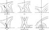Fig. 3. Simple submergence scenario for phase 2 cancellation with distributed sources (rather than point sources) of flux: (a) Magnetic field topology during phase 1a with submergence of the field below the separator; (b) Topology if reconnection ceases before submergence has been completed; (c) Magnetic topology if cancellation stops after large-scale submergence has finished; (d) Reconnection continuing when large-scale submergence has finished; (e) Close-up of the reconnection in the current sheet of (d), showing the production of a jet and small-scale submergence inside the current sheet; (f) Submergence during phase 1b.

First, we consider the scenario of simple flux submergence (Fig. 3) with flux sources that are diffuse (rather than highly concentrated). One possible cause of submergence is convective flow in the photosphere with a downflow at the submergence location. Another is the tension force of the magnetic field, provided it exceeds the magnetic pressure force and the polarities are small enough and close enough that the field lines are pulled down through the photosphere (Parker 1979, p. 136–141).

In Fig. 3a, we assume this process starts during phase 1a, when reconnection is still taking place in the atmosphere. This could lead to three possible configurations. First of all, cancellation could cease before the end of phase 1a, leaving the topology shown in Fig. 3b. Secondly, it could continue until the end of phase 1a (Fig. 3c), leaving behind two polarities that can further cancel. Thirdly, the field below the separator could fully submerge before reconnection at the separator is completed. Then, the lower end of the separator current sheet reaches the photosphere, separating the remaining magnetic flux of the two polarities (Fig. 3c). Reconnection continues inside the current sheet, accelerating a jet upwards and submerging flux downwards (Fig. 3d). Eventually, the cancellation leaves behind magnetic flux of magnitude F − F_p, with the topology shown in Fig. 1g. Simple submergence can also occur during phase 1b, as indicated in Fig. 3f. In this case, the cancellation, again, eventually leaves behind magnetic flux of magnitude F − F_p (Fig. 1g).

The second scenario by which cancellation phase 2 can occur is through the formation of a flux rope or mini-filament, alongside the flux submergence discussed above. When this process starts during phase 1b (Fig. 4a), the new feature is the formation of a current sheet above the polarity inversion line that lies between the two polarities. Converging motions at the current sheet drive reconnection which forms a region of closed magnetic field lines in two dimensions or a magnetic island.

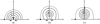Fig. 4. Flux rope scenario for phase 2 cancellation during phase 1b with distributed sources: (a) Magnetic field topology during phase 1b, with converging motions creating a current sheet; (b) Formation of flux rope containing a mini-filament and submergence of the field; (c) Build-up of flux rope and beginning of an eruption.

If there is also a magnetic component out of the plane, that island represents a section across a twisted magnetic flux rope. Since reconnection takes place low in the atmosphere, the island or flux rope will be filled with cool plasma, which may be referred to as a ‘mini-filament. As reconnection proceeds, the flux rope containing a mini-filament will rise up and expand (e.g. Sterling et al. 2015, 2016, 2020; Sterling & Moore 2016). Also, reconnection will submerge magnetic flux down through the photosphere within the current sheet and so cancel part of the initial flux (Fig. 4b). As the flux rope is built up by reconnection, more and more flux will be cancelled and submerged (Fig. 4c). Eventually, the twisted flux rope can erupt, together with jets of cool and hot plasma. The topology of such an eruption is further discussed below.

A flux rope can similarly be formed during phase 1a (Fig. 5a). In order to erupt, the flux rope will press up against the overlying separator and form a current sheet above the flux rope, at which the flux rope will reconnect (Fig. 5b). This will lead to more heating and jet production, and will allow the flux rope and the cool mini-filament to erupt along the inclined fieldlines, inducing twist by the reconnection between the flux rope with the untwisted field. Reconnection below the flux rope will assist the eruption, create an arcade field that can potentially submerge, while separating the erupting field from the non-erupting field via separatrix surfaces (Fig. 5c). The erupting flux rope will fully diffuse inside the external field (Fig. 5d) and the field will eventually relax. Further submergence will ultimately produce the topology in Fig. 1f.

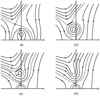Fig. 5. Flux rope scenario for phase 2 cancellation during phase 1a: (a) Magnetic field topology during phase 1a, with converging motions creating a current sheet; (b) Formation of flux rope containing a mini-filament and submergence of the field; (c) Reconnection of the flux rope at the overlying separator; (d) Topology after the flux rope erupts and diffuses.

An interesting point about phase 2 cancellation concerns the role of the plasma β (the ratio of plasma to magnetic pressure) in the later evolution of the system. As the magnetic field strength progressively decreases, the local plasma β could become higher than unity, allowing the gas pressure forces to dominate and change the behaviour of the system. For example, a small-scale photospheric high-β mini-filament would not necessarily erupt, but could be pushed around by the convective motions and eventually fragment or submerge by convective downdrafts.

2.3. Energy release during phase 1

2.3.1. Magnetic field strength (B_i) of the inflowing plasma

At this point, we focus on phase 1a reconnection. During phase 1a, a current sheet of length, L, forms at the location of the separator, where reconnection is driven (Fig. 1h). To estimate the energy release during this process, we first need to find the input magnetic field strength at the entrance to the current sheet. To do so, we linearise the magnetic field and start with a two-dimensional current sheet before applying the correction that was discovered in Paper I for a three-dimensional sheet.

Since the two polarities are of unequal flux, the current sheet is, unlike the case considered in Paper I, generally inclined. To simplify the analysis, we employ a coordinate system (x′,z′) for the inclined current sheet centred around (x_s, z_s), as shown in Fig. 6, where z′ is directed along the sheet and x′ is normal to it. Near the sheet, the magnetic field can then be written as

$$\begin{array}{c}\hfill B_{z^{\prime }}+i{B}_{x^{\prime }}=k{({Z^{\prime }}^2+{\left(\frac{L}{2}\right)}^2)}^{1/2},\end{array}$$(8)

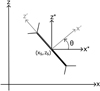Fig. 6. Coordinate system for the current sheet (x′,z′) and the unrotated coordinate system (x*, z*) centred around (xs, zs).

in terms of the complex variable Z′ = x′+iz′. For Z′ ≫ L, this becomes B_z′ + iB_x′ = kZ′, and so

$$\begin{array}{c}\hfill \left[\begin{array}{c}{B}_{x^{\prime }}\\ B_{z^{\prime }}\\ \end{array}\right]=k\left[\begin{array}{c}{z}^{\prime }\\ x^{\prime }\\ \end{array}\right].\end{array}$$

The original coordinates are (x, z), which become (x^*, z^*) when translated to the centre (x_s, z_s) of the current sheet, so that x = x_s + x^* and z = z_s + z^*. Then the coordinates (x^*, z^*) are rotated through an angle θ to give the current sheet coordinates (x′,z′), as in Fig. 6. The relation between the magnetic field components in the two latter coordinate systems is determined by using the rotation matrix (R_θ) as

$$\begin{array}{c}\hfill \left[\begin{array}{c}{B}_{x^{\ast }}\\ B_{z^{\ast }}\\ \end{array}\right]=R_{\theta }^T\left[\begin{array}{c}{B}_{x^{\prime }}\\ B_{z^{\prime }}\\ \end{array}\right]=k{R}_{\theta }^T\left[\begin{array}{cc}0& 1\\ 1& 0\\ \end{array}\right]R_{\theta }\left[\begin{array}{c}{x}^{\ast }\\ z^{\ast }\\ \end{array}\right]=k\left[\begin{array}{cc}sin2\theta & cos2\theta \\ cos2\theta & -sin2\theta \\ \end{array}\right]\left[\begin{array}{c}{x}^{\ast }\\ z^{\ast }\\ \end{array}\right].\end{array}$$

By setting a = ksin2θ and b = kcos2θ, the field components become

$$\begin{array}{c}\hfill \left[\begin{array}{c}{B}_{x^{\ast }}\\ B_{z^{\ast }}\\ \end{array}\right]=k\left[\begin{array}{cc}a& b\\ b& -a\\ \end{array}\right]\left[\begin{array}{c}{x}^{\ast }\\ z^{\ast }\\ \end{array}\right]\end{array}$$(9)

with

$$\begin{array}{c}\hfill k^2=a^2+b^2.\end{array}$$(10)

In the vicinity of the current sheet, where x^* ≈ 0 and z^* ≈ 0, the inflow magnetic field is found from Eq. (8) to be

$$\begin{array}{c}\hfill B_i=\frac{1}{2}kL=\frac{1}{2}\sqrt{a^2+b^2}L.\end{array}$$(11)

Next, we need to find the values of a and b in terms of the separatrix location (x_s, z_s) and the source half-separation (d). This can be accomplished by linearising either B_x or B_z in the vicinity of the current sheet using Eq. (3) and then comparing with Eq. (9). The z-component of Eq. (3) is

$$\begin{array}{c}\hfill 2B_z=\frac{z}{r_1^3}-F_p\frac{z}{r_2^3},\end{array}$$(12)

which may be linearised around the separator by setting x = x_s + ϵ₁ and z = z_s + ϵ₂, where ϵ₁ ≪ x_s and ϵ₂ ≪ z_s. We first note that

$$\begin{array}{cc}\hfill \frac{1}{r_1^3}& \approx \frac{1}{r_{1s}^3}(1-3\frac{x_s-d}{r_{1s}^2}{ϵ}_1-3\frac{z_s}{r_{1s}^2}{ϵ}_2),\hfill \\ \hfill \frac{1}{r_2^3}& \approx \frac{1}{r_{2s}^3}(1-3\frac{x_s+d}{r_{2s}^2}{ϵ}_1-3\frac{z_s}{r_{2s}^2}{ϵ}_2),\hfill \end{array}$$

where

$$\begin{array}{c}\hfill r_{1s}=\sqrt{{(x_s-d)}^2+z_s^2}\mathrm{and}{r}_{2s}=\sqrt{{(x_s+d)}^2+z_s^2}.\end{array}$$(13)

Then, the linearised B_z near the separator, may be written, after using Eq. (4), as

$$\begin{array}{c}\hfill B_z={ϵ}_1[-\frac{3}{2}{z}_s(\frac{x_s-d}{r_{1s}^5}-F_p\frac{x_s+d}{r_{2s}^5})]+{ϵ}_2[-\frac{3}{2}{z}_s^2(\frac{1}{r_{1s}^5}-F_p\frac{1}{r_{2s}^5})].\end{array}$$(14)

However, Eq. (9) implies that B_z = b(x − x_s)−a(z − z_s), which may be compared with Eq. (14) to give the values of a and b as

$$\begin{array}{c}\hfill a=\frac{3}{2}{z}_s^2(\frac{1}{r_{1s}^5}-F_p\frac{1}{r_{2s}^5})\mathrm{and}b=-\frac{3}{2}{z}_s(\frac{x_s-d}{r_{1s}^5}-F_p\frac{x_s+d}{r_{2s}^5}).\end{array}$$(15)

Therefore, when the current sheet is treated as a two-dimensional structure, the magnetic field strength of the plasma flowing into the current sheet is given by Eq. (11) with a and b given by Eq. (15).

Since the current sheet here is instead a three-dimensional structure, we now need to apply the correction derived in Paper I to the above two-dimensional result. The result is that the inflow magnetic field near the toroidal sheet is given, according to Eq. (11), by the $\frac{1}{2}kL$ from the two-dimensional linearisation times a correction factor associated with the curvature of the current, namely,

$$\begin{array}{c}\hfill B_i=\frac{1}{2}kL(1-0.2757ϵ{log}_eϵ),\end{array}$$

where k is now given by Eq. (10) and ϵ = L/(2R₀) ≪ 1. Therefore, the magnetic field strength of the plasma flowing into the current sheet during reconnection in phase 1a will be

$$\begin{array}{c}\hfill B_i=\frac{1}{2}L\sqrt{a^2+b^2}(1-0.2757ϵ{log}_eϵ),\end{array}$$(16)

where a and b are given by Eq. (15). We note that R₀ is the radius of the toroidal current, and so it is the length of the line segment connecting the midpoint of the two converging polarities, (x, z) = (0, 0), and the separator (x_s, z_s), that is,

$$\begin{array}{c}\hfill R_0=\sqrt{x_s^2+z_s^2}.\end{array}$$(17)

2.3.2. Rate of change of flux below the separator and inflow velocity

We calculate v_i from the rate of change (dψ/dt) of magnetic flux through the semicircle of radius, z_s, out of the plane of Fig. 1h. This rate of change of flux becomes, after using E + v × B = 0 and Faraday’s Law,

$$\begin{array}{c}\hfill \frac{\mathrm{d}\psi }{\mathrm{d}t}=-\pi z_{s}E=\pi z_s{v}_i{B}_i.\end{array}$$(18)

Then, ψ may be calculated from the magnetic flux below z_S through the semicircle, namely,

$$\begin{array}{c}\hfill \psi ={\displaystyle {\int }_0^{z_s}\pi z{B}_x(x_s,z)\mathrm{d}z.}\end{array}$$

Taking its time derivative gives

$$\begin{array}{cc}\hfill \frac{\mathrm{d}\psi }{\mathrm{d}t}& =\pi z_s{B}_x(x_s,z_s)\frac{\mathrm{d}{z}_s}{\mathrm{d}t}\hfill \\ \hfill & +\pi \frac{\mathrm{d}{x}_s}{\mathrm{d}d}{\displaystyle {\int }_0^{z_s}z\frac{\partial B_x}{\partial x_s}\mathrm{d}z+\pi {\int }_0^{z_s}z\frac{\partial B_x}{\partial d}\mathrm{d}z,}\hfill \end{array}$$

using that v₀ = dd/dt = 1 is the convergence speed in dimensionless form. The first term of the above equation vanishes, since B_x(x_s, z_s) = 0, whereas the integrals can be calculated directly, and, following simplifications based on Eq. (4) at the separator, they become

$$\begin{array}{cc}& {\displaystyle {\int }_0^{z_s}z\frac{\partial B_x}{\partial x_s}\mathrm{d}z=0,\mathrm{and}{\int }_0^{z_s}z\frac{\partial B_x}{\partial d}\mathrm{d}z=F_p\frac{z_s^2}{r_{2s}^3},}\hfill \end{array}$$

and so the rate of change of flux is

$$\begin{array}{c}\hfill \frac{\mathrm{d}\psi }{\mathrm{d}t}=\pi F_p\frac{z_s^2}{r_{2s}^3},\end{array}$$(19)

where dψ/dt has been normalised with respect to $d_0^2{B}_0$. Technically, the above solution has a singular point when the separator is located above the minor polarity, but for practical purposes, this does not cause any issues (see Appendix A).

Having found dψ/dt, using Eq. (18), the inflow velocity then becomes

$$\begin{array}{c}\hfill v_i=F_p\frac{z_s}{r_{2s}^3}\frac{2}{L}\frac{1}{\sqrt{a^2+b^2}}{(1-0.2757ϵ{log}_eϵ)}^{-1}.\end{array}$$(20)

2.3.3. Energy release

The nature of the reconnection will dictate the length (L) of the current sheet and therefore the plasma inflow speed. For example, a Sweet-Parker reconnection would result in a long diffusive region and a slow inflow of plasma. For fast reconnection, the diffusion region is much shorter and the inflow speed is larger, a fraction of the local Alfvén speed (see discussion in Priest et al. 2018; Syntelis et al. 2019), but the current sheet includes the slow-mode shock waves, since most of the energy conversion takes place at them.

Following Priest et al. (2018), the rate of conversion of inflowing magnetic energy into heat can be written as

$$\begin{array}{c}\hfill \frac{\mathrm{d}W}{\mathrm{d}t}=0.8\frac{v_i{B}_i^2}{\mathrm{\mu }}L\pi z_s,\end{array}$$(21)

where L is determined from Eq. (20) once v_i has been determined by the nature of the reconnection. For a fast reconnection, the inflow speed will be a fraction (α, say) of the local Alfvén speed, and so

$$\begin{array}{c}\hfill v_i=\alpha v_{\mathit{Ai}},\end{array}$$

where v_Ai is the Alfvén velocity of the inflowing plasma and α is typically 0.1. In dimensional form, we write v_Ai = v_A0B_i/B₀, where ${\mathit{v}}_{A0}=B_0/\sqrt{\mathrm{\mu }{\rho }_i}$. In dimensionless form, this becomes v_Ai = v_A0B_i, and so the inflow speed is

$$\begin{array}{c}\hfill v_i=\alpha \frac{B_i}{M_{A0}},\end{array}$$(22)

in terms of the Mach Alfvén number M_A0 = v₀/v_A0 (where v₀ = 1 in dimensionless form). After substituting this expression into Eq. (20) and using Eq. (16) for B_i, the length of the current sheet becomes

$$\begin{array}{c}\hfill L={\left(\frac{M_{A0}}{\alpha }\frac{F_p}{{\kappa }^2}\frac{z_s}{r_{2s}^3}\right)}^{1/2},\end{array}$$(23)

where

$$\begin{array}{c}\hfill \kappa =\frac{1}{2}\sqrt{a^2+b^2}(1-0.2757ϵ{log}_eϵ).\end{array}$$(24)

Through ϵ, the expression for L contains terms L/2R₀ on the right-hand side of the equation. So, to compute L, Eq. (23) can be solved numerically for L. Alternatively, since L/2R₀ ≪ 1 the terms in L/2R₀ can be treated as corrections, so that

$$\begin{array}{cc}\hfill L& =\sqrt{\frac{M_{A0}}{\alpha }\frac{4}{a^2+b^2}{F}_p\frac{z_s}{r_{2s}^3}}{(1-0.2757ϵ{log}_eϵ)}^{-1}\hfill \\ \hfill & \approx L_0{(1-0.2757{ϵ}_0{log}_e{ϵ}_0)}^{-1},\hfill \end{array}$$(25)

where ϵ₀ = L₀/(2R₀) and $L_0=\sqrt{4M_{A0}{F}_p/[\alpha (a^2+b^2)](z_s/r_{2s}^3)}$.

This method of calculating L produces the same values as solving Eq. (23) numerically for L, except for regions close to the critical points, which are discussed below. Then, after substituting for v_i (Eq. (22)), L (Eq. (23)), and B_i (Eq. (16)) into Eq. (21), the rate of energy conversion to heat during phase 1a finally becomes

$$\begin{array}{c}\hfill \frac{\mathrm{d}W}{\mathrm{d}t}=0.8\pi \frac{M_{A0}}{\alpha }\frac{F_p^2}{\kappa }\frac{z_s^3}{r_{2s}^6},\end{array}$$(26)

where dW/dt is normalised with respect to $v_0{B}_0^2{d}_0^2$/μ.

We note that by setting F_p = 1, all our expressions are reduced to the expressions that describe the cancellation of two equal fluxed, described in Paper I.

2.3.4. Behaviour near the critical points

The expressions for L, B_i, dψ/dt and dW/dt do not always behave well near critical points (z_s → 0, when d → d_c1 or d → d_c2). Some of these quantities tend to infinity near the critical points for some values of F_p. This issue arises when the current sheet length becomes comparable with the distance of the separator from the photosphere and the linearisation fails. A detailed discussion on the behaviour near the critical points can be found in Appendix B.

In the numerical analysis of the analytical solutions presented in the next section, we calculate the quantities only for L₀ < R₀, cutting off the unphysical solution around the critical points. In reality, near the critical points, each of L, dψ/dt, dW/dt should to tend to zero and produce only a small extra energy release. In fact, our dW/dt solution tends to infinity only for F_p = 1, but due to the behaviour of L, we cut off the solution at the linear regime for all values of F_p.

3. Discussion

Figures 7a–c show the values of dψ/dt, L, dW/dt for α = 0.1 and M_A0 = 0.01 for different values of the fluxes (F_p) of the minority polarity. The curves are cut off near d = d_c1 and d = d_c2, where the analysis fails since it implies unphysically that L > R₀. Minority polarities with smaller flux release the energy at smaller separations, d, since the separator quickly returns to the photosphere.

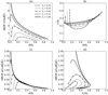Fig. 7. Physical parameters of cancellation for v0 = 1, α = 0.1 and MA0 = 0.01. (a) Rate of change (dψ/dt) of flux below the separator, for different values of the minority flux (Fp). (b) Length (L) of the current sheet for different values of Fp. (c) Rate (dW/dt) of energy conversion to heat for different values of Fp. (d) dW/dt for different values of Fp as a function of the null height zs. In (b)–(d), the solution above L0 > R0 is cut off.

These plots may be used to identify the height where the maximum dW/dt occurs for different values of F_p. For the cancellation of small magnetic fragments, we can adopt an atmospheric field of, say, B₀ = 10 G, a major polarity of F = 10¹⁹ Mx and a speed of v₀ = 1 km s⁻¹, which gives d₀ = 5.6 Mm, and $v_0{B}_0^2{d}_0^2/(4\pi )=2.5\times {10}^{23}$ erg s⁻¹. Therefore, for F_p between 10¹⁸ and 10¹⁹ Mx, the maximum energy release rate occurs at heights of about 1.2−1.8 Mm, that is, in the chromosphere (Fig. 7d). The maximum height (max(z_s)) of a separator during the reconnection is 1.8−3.5 Mm, while the maximum rate of energy release is 1.0−9.5 × 10²³ erg s⁻¹. The total energy release during phase 1 of the cancellation may then be estimated as:

$$\begin{array}{c}\hfill E={\displaystyle \int }\frac{\mathrm{d}W}{\mathrm{d}t}\frac{\mathrm{d}t}{\mathrm{d}d}\mathrm{d}d=\frac{1}{v_0}{\displaystyle \int }\frac{\mathrm{d}W}{\mathrm{d}t}\mathrm{d}d,\end{array}$$

with a range of 1.6−4.2 × 10²⁶ erg. A Mach number of M_A0 = 0.1 instead increases by a factor of 10 the energy rates and total energies released at the same heights. For the cancellation of smaller magnetic fragments with a majority polarity of, say, F = 10¹⁸ Mx, the flux interaction distance becomes d₀ = 1.8 Mm, and $v_0{B}_0^2{d}_0^2/(4\pi )=2.5\times {10}^{22}$ erg s⁻¹. Therefore, for F_p between 10¹⁷ − 10¹⁸ Mx, the maximum energy release rate occurs at heights of 0.4−0.6 Mm, namely, in the photosphere and chromosphere. The maximum height (max(z_s)) of the separator during reconnection is 0.6−1.1 Mm. The maximum rate of energy release is 1−9.5 × 10²² erg s⁻¹, whereas the total energy released during phase 1 cancellation is 5.2−10.3 × 10²⁴ erg. Again, M_A0 = 0.1 gives an order of magnitude higher energy rates and total energies.

Estimates for the energy release during phase 2 can be found in Paper I. Overall, the cancellation of small magnetic fragments produces energetic events typical of nanoflares. We note that larger flux elements will probably consist of many finer intense flux tubes with persistent flux cancellation. In addition, during cancellation, larger flux elements can break into smaller polarities and release the energy in smaller segments. It is also important to remember that cancellation typically occurs in fits and starts. Thus, the total energy release can take place as a series of nanoflares or microflares over an extended time of hundreds or thousands of seconds, as has been reported in some observations and simulations of flux cancellation, such as Peter et al. (2019) and Park (2020).

4. Conclusions

Recent observations have reported that magnetic flux cancellation occurs at a significantly higher rate than previously thought. Therefore, the energy released during flux cancellation can potentially be the dominant factor in heating the atmosphere and accelerating various kinds of jets in different parts of the solar atmosphere. The aim of the present paper has been to develop further the basic theory for energy release driven by flux cancellation.

In Priest et al. (2018), we developed a model for energy release during the cancellation of two polarities of equal flux in the presence of a uniform horizontal magnetic field. In Paper I, we extended that theory by treating the current sheet as a series of toroidal three-dimensional current sheets, instead of two-dimensional sheets. In this paper, we take the next step and extend the model to the case of convergence and cancellation of two polarities of unequal flux.

We have found that cancellation occurs in two phases. During phase 1, reconnection occurs at a separator that first moves up and then descends back down to the photosphere. We derived estimates for the energy release and the height where this occurs and found that it is released during flux cancellation in the form of nanoflares. An important new feature of this model is that when the separator moves back to the photosphere and the first phase of reconnection ceases, the two polarities have not yet fully cancelled out. Instead, the remaining magnetic flux cancels by the submergence of the field during phase 2, with reconnection occurring in or just above the photosphere between the two cancelling regions. This process can occur either via a simple reconnection and submergence of the field connecting the two polarities or by the formation and eruption of a flux rope containing a mini-filament created between the two cancelling polarities.

In our previous numerical models for the case of two cancelling polarities (Syntelis et al. 2019; Syntelis & Priest 2020), we found that several types of reconnection-driven outflow can be produced during the cancellation. Depending on the height where the separator is located, reconnection can drive a wide variety of jets, whose density and temperature can vary significantly, from very cool (10 000 K) to very hot (2 MK). Similar jets would be produced during phase 1 for the general case of unequal fluxes discussed in this paper. During phase 2, reconnection-driven jets can also form at a current sheet that extends up from the photosphere either following the simple submergence of the field of the magnetic domain connecting the two cancelling polarities or following a mini-filament eruption. In addition, the eruption of a mini-filament can form a cool eruption-driven jet, which may be more twisted than normal reconnection-driven jets. In the future, we would like to consider other flux geometries and use detailed numerical models to validate and advance the basic theory presented here.

Acknowledgments

ERP is grateful for helpful suggestions and hospitality from Pradeep Chitta, Hardi Peter, Sami Solanki and other friends in MPS Göttingen, where this research was initiated. P.S. acknowledge support by the ERC synergy grant “The Whole Sun”.

References

Appendix A: Rate of change of flux

In Sect. 2.3.2 we calculated the rate of change of flux below the separator, namely,

$$\begin{array}{c}\hfill \psi ={\displaystyle {\int }_0^{z_s}\pi z{B}_x(x_s,z)\mathrm{d}z.}\end{array}$$(A.1)

As the polarities converge, the separator moves towards and eventually passes over the minor polarity (Figs. 1b–e). What we really need is the rate of change of the flux (ψ_A < 0) in the domain that joins the source F to the source −F_p. Thus, when x_s > −d and the separator lies to the right of the source −F_p:

$$\begin{array}{c}\hfill {\psi }_A=\psi \mathrm{and}\frac{\mathrm{d}{\psi }_A}{\mathrm{d}t}=\frac{\mathrm{d}\psi }{\mathrm{d}t}.\end{array}$$

However, when x_s < −d and the separator lies to the left of the source −F_p, the flux calculated by Eq. (A.1) is:

$$\begin{array}{c}\hfill \psi =-{\psi }_B,\end{array}$$

in terms of the negative flux (ψ_B) coming in from the left to −F_p (Figs. 1c,d). However,

$$\begin{array}{c}\hfill {\psi }_A+{\psi }_B=-F_p,\end{array}$$

where F_p > 0, and so, for x_s < −d, the flux we seek is

$$\begin{array}{c}\hfill {\psi }_A=\psi -F_p.\end{array}$$

In other words, when x_s < −d, we need to subtract F_p from the graph for ψ. The result is that in both ranges for x_s,

$$\begin{array}{c}\hfill \frac{\mathrm{d}{\psi }_A}{\mathrm{d}t}=\frac{\mathrm{d}\psi }{\mathrm{d}t}.\end{array}$$

When x_s = −d and the separator lies above the minority polarity, ψ is discontinuous, but the derivatives are continuous.

To examine this further, we calculate the flux using Eq. (A.1) and find its derivative. We have:

$$\begin{array}{cc}\hfill \psi & ={\displaystyle {\int }_0^{z_s}\pi z{B}_x(x_s,z)\mathrm{d}z}\hfill \\ \hfill & =\frac{\pi }{2}{\displaystyle {\int }_0^{z_s}z[\frac{x_s-d}{{[{(x_s-d)}^2+z^2]}^{3/2}}-F_p\frac{x_s+d}{{[{(x_s+d)}^2+z^2]}^{3/2}}+2]\mathrm{d}z.}\hfill \end{array}$$

The first two integrals are

$$\begin{array}{c}\hfill I_1=-\frac{x_s-d}{{[{(x_s-d)}^2+z^2]}^{1/2}}-1\end{array}$$

and

$$\begin{array}{c}\hfill I_2=F_p\frac{x_s+d}{{[{(x_s+d)}^2+z^2]}^{1/2}}-F_p\mathrm{sign}(x_s+d),\end{array}$$

so the flux below the separator is

$$\begin{array}{cc}\hfill \psi =\frac{\pi }{2}[& -\frac{x_s-d}{{[{(x_s-d)}^2+z^2]}^{1/2}}+F_p\frac{x_s+d}{{[{(x_s+d)}^2+z^2]}^{1/2}}\hfill \\ \hfill & +z_s^2-1-F_p\mathrm{sign}(x_s+d)].\hfill \end{array}$$(A.2)

The resulting ψ is plotted in Fig. A.1 for different values of F_p and clearly demonstrates the jump in value at d = |x_s|. Provided x_s ≠ −d, the derivative of the above (and therefore the value of dψ_A/dt) is:

$$\begin{array}{c}\hfill \frac{\mathrm{d}\psi }{\mathrm{d}t}=\pi v_0{F}_p\frac{z_s^2}{r_{2s}^3},\end{array}$$(A.3)

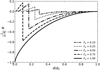Fig. A.1. Flux (ψ) below the separator as a function of d for different values of Fp, calculated from Eq. (A.2)

and so our previous solution (Eq. (19)) is indeed valid. When x_s = −d, we simply define dψ_A/dt to be the limit as x_s → −d of dψ/dt.

Appendix B: Behaviour near critical points

In this appendix, we extend the discussion in Sect. 2.3.4 on the behaviour of the solution near critical points.

To do so, we examine the behaviour of dψ/dt, L, and dW/dt approaching the critical points where z_s → 0 which happens as d → d_c1 and d → d_c2.

Case of F_p < 1

When z_s → 0, x_s approaches a constant non-zero value (Eq. (5) and Fig. 2c), while r_1s and r_2s also approach constant non-zero values (Eq. (13)). To examine the behaviour of L, we use Eq. (25). For z_s → 0, L₀ behaves as:

$$\begin{array}{c}\hfill L_0\propto z_s^{-1/2}\end{array}$$

since $a\propto z_s^2$ and b ∝ z_s. Therefore, L₀ will tend to infinity at the critical points. We may notice from Fig. B.1 that the linearisation fails when z_s (dashed black line) becomes comparable to the L₀ (solid black line). After that point the separator moves to the photosphere, and L₀ should tend to zero instead of infinity.

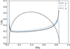Fig. B.1. Length (L0) of the current sheet without the 3D correction (solid black), the height of the separator zs (dashed black), and the length (L) of the current sheet with the 3D correction.

The remaining terms of L, namely,

$$\begin{array}{c}\hfill {(1-0.2757\frac{L_0}{2R_0}{log}_e\frac{L_0}{2R_0})}^{-1}\end{array}$$

tends to infinity when the denominator is zero, which is for L₀/(2R₀) ≈ 3.13, and eventually tends to zero when L₀ → ∞ as z_s → 0. This anomalous behaviour can be seen in Fig. B.1 (blue line). We note that the singularity appears only at the lower critical point.

The energy release dW/dt without the 3D correction term tends to zero around the critical points for F_p < 1. Estimating the behaviour of dW/dt is more challenging with the 3D correction term, but a numerical solution of the equation shows that dW/dt tends to zero before the correction term tends to infinity (Fig. B.2).

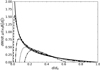Fig. B.2. Rate (dW/dt) of energy conversion to heat for different values of Fp, without cutting off the solution when L0 = R0.

The rate of change of flux dψ/dt (Eq. (19)) tends to zero around the critical points for F_p < 1.

Case of F_p = 1

When F_p = 1, x_s is always zero and the critical points occur for d = 0 or d = 1. Another important difference to the F_p < 1 case is that r_1s = r_2s = d^1/3, which for d = 0 tends to zero rather than a constant value. Therefore, the quantities that have terms like 1/r_2s, such as dψ/dt, need to be examined with care.

As d → 0, z_s ∝ d^1/3, the rate of change of flux behaves like $\text{d}\psi /\text{d}t\propto d^{-1/3}\propto z_s^{-1}$, and so the rate of change of flux tends to infinity for d = 0.

The length (L₀)of the current sheet may now be written as:

$$\begin{array}{c}\hfill L_0^2=\frac{4M_{A0}}{9\alpha }\frac{1}{\sqrt{1-d^{4/3}}},\end{array}$$(B.1)

which goes to infinity as d → 1. Using $z_s=\sqrt{d^{2/3}-d^2}=d^{1/3}\sqrt{1-d^{4/3}}$, we see that $L_0\propto z_s^{-1/2}$, similar to the F_p < 1 case.

The rate of energy conversion to heat for F_p = 1, without the 3D correction, is written as

$$\begin{array}{c}\hfill \frac{\mathrm{d}W}{\mathrm{d}t}=0.8\frac{2\pi }{3}\frac{M_{A0}}{\alpha }\frac{1-d^{4/3}}{d^{2/3}},\end{array}$$(B.2)

which goes to infinity for d = 0 as $\text{d}W/\text{d}t\propto d^{-2/3}\propto z_s^{-2}$.

All Figures

Fig. 1. Overall behaviour of the magnetic field during the approach of two oppositely directed photospheric polarities (stars) of flux, −Fp and F, (where |Fp|< |F|) are separated by a distance, 2d, and situated in an overlying uniform horizontal magnetic field (B0). The magnetic field is axisymmetric, shown here in a vertical (y = 0) plane. Dashed curves show separatrix magnetic field lines and solid curves indicate other magnetic field lines. The separator is marked by an unfilled dot, and null points with solid dots. The field is shown for (a) d > dc1, when the two sources are far apart, (b) d = dc1, when the nulls coalesce at the photosphere (z = 0) and a separator first appears, (c) dc2 < d < dc1 (phase 1a), when the separator arches above the surface, (d) dc2 < d < dc1 (phase 1a), when the separator has moved to the left of the flux source −Fp, (e) d = dc2, when the separator falls back down to the photosphere and becomes a second-order null, (f) 0 < d < dc2 (phase 1b), when the null has bifurcated into two null points moving away from each other, and (g) d = 0, when the two sources have coalesced, leaving behind the remaining magnetic fragment of flux (F − Fp). Panel h: notation used to describe the reconnection process at a current sheet of length L.

In the text

Fig. 2. Position of the separator during Phase 1. (a) Height (zs) of the separator as a function of the half-separation (d) for different values of the minority flux (Fp). The coloured points mark the locations of the maximum zs (green) and the critical points where zs = 0 for d = dc1 (blue) and d = dc2 (red). (b) Horizontal position (xs) of the separator as a function of d. (c) Positions (xs, zs) of the separator in the y = 0 plane as d varies for different values of Fp.

In the text

Fig. 3. Simple submergence scenario for phase 2 cancellation with distributed sources (rather than point sources) of flux: (a) Magnetic field topology during phase 1a with submergence of the field below the separator; (b) Topology if reconnection ceases before submergence has been completed; (c) Magnetic topology if cancellation stops after large-scale submergence has finished; (d) Reconnection continuing when large-scale submergence has finished; (e) Close-up of the reconnection in the current sheet of (d), showing the production of a jet and small-scale submergence inside the current sheet; (f) Submergence during phase 1b.

In the text

	Fig. 4. Flux rope scenario for phase 2 cancellation during phase 1b with distributed sources: (a) Magnetic field topology during phase 1b, with converging motions creating a current sheet; (b) Formation of flux rope containing a mini-filament and submergence of the field; (c) Build-up of flux rope and beginning of an eruption.
In the text

	Fig. 5. Flux rope scenario for phase 2 cancellation during phase 1a: (a) Magnetic field topology during phase 1a, with converging motions creating a current sheet; (b) Formation of flux rope containing a mini-filament and submergence of the field; (c) Reconnection of the flux rope at the overlying separator; (d) Topology after the flux rope erupts and diffuses.
In the text

	Fig. 6. Coordinate system for the current sheet (x′,z′) and the unrotated coordinate system (x*, z*) centred around (xs, zs).
In the text

Fig. 7. Physical parameters of cancellation for v0 = 1, α = 0.1 and MA0 = 0.01. (a) Rate of change (dψ/dt) of flux below the separator, for different values of the minority flux (Fp). (b) Length (L) of the current sheet for different values of Fp. (c) Rate (dW/dt) of energy conversion to heat for different values of Fp. (d) dW/dt for different values of Fp as a function of the null height zs. In (b)–(d), the solution above L0 > R0 is cut off.

In the text

	Fig. A.1. Flux (ψ) below the separator as a function of d for different values of Fp, calculated from Eq. (A.2)
In the text

	Fig. B.1. Length (L0) of the current sheet without the 3D correction (solid black), the height of the separator zs (dashed black), and the length (L) of the current sheet with the 3D correction.
In the text

	Fig. B.2. Rate (dW/dt) of energy conversion to heat for different values of Fp, without cutting off the solution when L0 = R0.
In the text

References

- Chen, Y., Tian, H., Peter, H., et al. 2019, ApJ, 875, L30 [NASA ADS] [CrossRef] [Google Scholar]
- Chitta, L. P., Peter, H., Solanki, S. K., et al. 2017, ApJS, 229, 4 [NASA ADS] [CrossRef] [Google Scholar]
- Chitta, L. P., Peter, H., & Solanki, S. K. 2018, A&A, 615, L9 [NASA ADS] [CrossRef] [EDP Sciences] [Google Scholar]
- Harvey, K. L. 1985, ApJ, 38, 875 [Google Scholar]
- Hong, J., Ding, M. D., & Cao, W. 2017, ApJ, 838, 101 [NASA ADS] [CrossRef] [Google Scholar]
- Huang, Z., Mou, C., Fu, H., et al. 2018, ApJ, 853, L26 [Google Scholar]
- Huang, Z., Li, B., & Xia, L. 2019, Sol.-Terr. Phys., 5, 58 [Google Scholar]
- Longcope, D. W. 1998, ApJ, 507, 433 [NASA ADS] [CrossRef] [Google Scholar]
- Low, B. C. 1991, ApJ, 381, 295 [Google Scholar]
- Martin, S. F., Livi, S., & Wang, J. 1985, ApJ, 38, 929 [Google Scholar]
- Ortiz, A., Hansteen, V. H., Nóbrega-Siverio, D., & van der Voort, L. R. 2020, A&A, 633, A58 [CrossRef] [EDP Sciences] [Google Scholar]
- Panesar, N. K., Sterling, A. C., Moore, R. L., & Chakrapani, P. 2016, ApJ, 832, L7 [NASA ADS] [CrossRef] [Google Scholar]
- Panesar, N. K., Sterling, A. C., Moore, R. L., et al. 2019, ApJ, 887, L8 [Google Scholar]
- Park, S.-H. 2020, ApJ, 897, 49 [Google Scholar]
- Parker, E. N. 1979, Cosmical Magnetic Fields. Their Origin and Their Activity, The International Series of Monographs on Physics (Oxford: Clarendon Press) [Google Scholar]
- Peter, H., Tian, H., Curdt, W., et al. 2014, Science, 346 [CrossRef] [Google Scholar]
- Peter, H., Huang, Y. M., Chitta, L. P., & Young, P. R. 2019, A&A, 628, A8 [CrossRef] [EDP Sciences] [Google Scholar]
- Priest, E. R. 1987, in The Role of Fine-Scale Magnetic Fields on the Structure of the Solar Atmosphere, eds. A. W. E. Schroter, & M. Vazquez (Camb, Univ. Press.), 297 [Google Scholar]
- Priest, E. R., Chitta, L. P., & Syntelis, P. 2018, ApJ, 862, L24 [Google Scholar]
- Priest, E. R., & Syntelis, P. 2021, A&A, 647, A31 [EDP Sciences] [Google Scholar]
- Reid, A., Mathioudakis, M., Doyle, J. G., et al. 2016, ApJ, 823, 110 [NASA ADS] [CrossRef] [Google Scholar]
- Rezaei, R., & Beck, C. 2015, A&A, 582, A104 [NASA ADS] [CrossRef] [EDP Sciences] [Google Scholar]
- Şahin, S., Yurchyshyn, V., Kumar, P., et al. 2019, ApJ, 873, 75 [Google Scholar]
- Samanta, T., Tian, H., Yurchyshyn, V., et al. 2019, Science, 366, 890 [Google Scholar]
- Smitha, H. N., Anusha, L. S., Solanki, S. K., & Riethmüller, T. L. 2017, ApJS, 229, 17 [Google Scholar]
- Solanki, S. K., Barthol, P., Danilovic, S., et al. 2010, ApJ, 723, L127 [Google Scholar]
- Solanki, S. K., Riethmüller, T. L., Barthol, P., et al. 2017, ApJS, 229, 2 [Google Scholar]
- Sterling, A. C., & Moore, R. L. 2016, ApJ, 828, L9 [Google Scholar]
- Sterling, A. C., Moore, R. L., Falconer, D. A., & Adams, M. 2015, Nature, 523, 437 [Google Scholar]
- Sterling, A. C., Moore, R. L., Falconer, D. A., et al. 2016, ApJ, 821, 100 [Google Scholar]
- Sterling, A. C., Moore, R. L., Samanta, T., & Yurchyshyn, V. 2020, ApJ, 893, L45 [Google Scholar]
- Syntelis, P., & Priest, E. R. 2020, ApJ, 891, 52 [NASA ADS] [CrossRef] [Google Scholar]
- Syntelis, P., Priest, E. R., & Chitta, L. P. 2019, ApJ, 872, 32 [NASA ADS] [CrossRef] [Google Scholar]
- Tian, H., Xu, Z., He, J., & Madsen, C. 2016, ApJ, 824, 96 [CrossRef] [Google Scholar]
- Tiwari, S. K., Alexander, C. E., Winebarger, A. R., & Moore, R. L. 2014, ApJ, 795, L24 [Google Scholar]
- Ulyanov, A. S., Bogachev, S. A., Loboda, I. P., Reva, A. A., & Kirichenko, A. S. 2019, Sol. Phys., 294, 128 [Google Scholar]
- van Ballegooijen, A. A., & Martens, P. C. H. 1989, ApJ, 343, 971 [Google Scholar]
- van der Voort, L. R., Pontieu, B. D., Scharmer, G. B., et al. 2017, ApJ, 851, L6 [NASA ADS] [CrossRef] [Google Scholar]
- Vissers, G. J. M., van der Voort, L. H. M. R., & Rutten, R. J. 2013, ApJ, 774, 32 [NASA ADS] [CrossRef] [Google Scholar]
- Watanabe, H., Vissers, G., Kitai, R., Rouppe van der Voort, L., & Rutten, R. J. 2011, ApJ, 736, 71 [NASA ADS] [CrossRef] [Google Scholar]