| Issue |
A&A
Volume 649, May 2021
|
|
|---|---|---|
| Article Number | A36 | |
| Number of page(s) | 9 | |
| Section | The Sun and the Heliosphere | |
| DOI | https://doi.org/10.1051/0004-6361/202140314 | |
| Published online | 07 May 2021 | |
Flute oscillations of cooling coronal loops with variable cross-section
1
Solar Physics and Space Plasma Research Centre (SP2RC), School of Mathematics and Statistics, University of Sheffield, Sheffield S3 7RH, UK
e-mail: robertus@sheffield.ac.uk
2
School of Build Environment, Engineering and Computing, Leeds Beckett University, Leeds LS1 3HE, UK
3
Department of Astronomy, Eötvös Loránd University, Pázmány Péter sétány 1/A, 1117 Budapest, Hungary
4
Gyula Bay Zoltán Solar Observatory (GSO), Hungarian Solar Physics Foundation (HSPF), Petőfi tér 3., Gyula 5700, Hungary
Received:
11
January
2021
Accepted:
17
February
2021
We consider fluting oscillations in a thin straight expanding magnetic flux tube in the presence of a background flow. The tube is divided into a core region that is wrapped in a thin transitional region, where the damping takes place. The method of multiple scales is used for the derivation of the system of governing equations. This system is applicable to study both standing and propagating waves. Furthermore, the system of equations is obtained for magnetic tubes with a sharp boundary. An adiabatic invariant is derived using the Wentzel-Kramer-Brillouin method for a magnetic flux tube with slowly varying density, and the theoretical results are then used to investigate the effect of cooling on flute oscillations of a curved flux tube semi-circlular in shape. We have analysed numerically the dependencies of the dimensionless amplitude for a range of values of the expansion factor and the ratio of internal to external plasma densities at an initial time. We find that the amplitude increases due to cooling and is higher for a higher expansion factor. Higher values of the wave number lead to localisation of the oscillation closer to the boundary. Finally, we show that the higher the value of the ratio of internal to external plasma densities, the higher the amplification of oscillation due to cooling. Therefore, we conclude that the wave number, density ratio, and the variation of tube expansion are all relevant parameters in the cooling process of an oscillating flux tube.
Key words: magnetohydrodynamics (MHD) / plasmas / Sun: corona / Sun: oscillations / waves
© ESO 2021
1. Introduction
The presence of a complex magnetic field, which makes the plasma highly structured and dynamic, dominates the dynamics in a wide range of regions of the solar atmosphere. Improvements in solar telescope technology over the past two decades have enabled detections of a myriad of periodic perturbations in a wide range of magnetic structures (see, e.g., Banerjee et al. 2007, and Tomczyk et al. 2007), that are often described in terms of magnetohydrodynamic (MHD) waves. MHD wave theory is a powerful tool to be exploited for plasma diagnostics of these structures, known as solar magneto-seismology (SMS; see reviews by Erdélyi 2006a; 2006b; Andries et al. 2009, and Ruderman & Erdélyi 2009). SMS combines the measured characteristics of waves with theoretical MHD modelling, and makes it possible to determine waveguide parameters that are hard to measure directly, like the coronal magnetic field strength (Nakariakov & Ofman 2001; Erdélyi & Taroyan 2008, and Kuridze et al. 2019).
One of the first approaches used for modelling solar atmospheric waveguides was based on representing the magnetic flux as a straight homogeneous magnetic cylinder (see, e.g., Ryutov & Ryutova 1976, and Edwin & Roberts 1983). Since then, more complex and more realistic models have been developed (for recent reviews, see, e.g., Nakariakov & Verwichte 2005, Ruderman & Erdélyi 2009 and Nakariakov et al. 2016).
It is customary to categorise the wave modes in a magnetic flux tube depending on the azimuthal wavenumber m (see, e.g., Edwin & Roberts 1983), where m = 0 corresponds to sausage waves, modes with m = 1 are the kink modes, and modes with m ≥ 2 are called the fluting modes. The properties of sausage and kink modes have been studied in a significant number of articles; on the contrary, fluting modes are not getting sufficient attention which can probably be explained by the absence of observations associated with fluting modes. A reason for the lack of observed detection of these modes may be related to the need of high spatial and temporal resolution, where the former is not that easy to achieve.
Nevertheless, there is a great interest in investigating the fluting modes with a theoretical approach as analysing these modes may provide further insights into the sub-resolution structure of a waveguide, and into their high potentials contributing to heating. An initial insight, popular today, into the properties of the oscillations of the flux tube with fluting modes is given by Edwin & Roberts (1983); a homogeneous flux tube was studied, and it was shown how the sausage, kink, and fluting modes behave under solar atmospheric circumstances. However, Ruderman et al. (2017), among others, has theoretically revealed for the kink modes that the dispersion is rather different for a non-homogeneous flux tube with plasma flows even in the thin tube and thin boundary approximation. Moreover, numerical experiments and contemporary theory suggest that the kink and fluting waves could couple in a non-linear fashion (see, e.g., Ruderman et al. 2010; Ruderman 2017, and Terradas et al. 2018). Another interesting aspect is that high azimuthal wavenumbers could be determinant in the cause of the Kelvin-Helmholtz instability (see, e.g., Terradas et al. 2008, Antolin et al. 2014, and Magyar & Van Doorsselaere 2016). As a result, additional investigation of the behaviour of the fluting oscillations could complement the analysis of the sausage and kink modes. Examples of the latter are Pascoe et al. (2016, 2017), Nelson et al. (2019), and Shukhobodskaia et al. (2021), among others, where significant development has lead to a better understanding of kink oscillations of coronal loops, although contemporary theory is still unable to perfectly match the observed oscillation patterns.
In this work, we further extend the study of oscillations of coronal loops. Coronal loops with elliptical cross-sections and a constant density profile have been studied previously in both cold (Ruderman 2003), and finite-β (Erdélyi & Morton 2009) plasmas. Fluting oscillation, central to the current paper, in the absence of background flows and magnetic flux tube expansion was studied comprehensively by Soler (2017). In our work we now consider fluting modes in expanding cylindrical flux tubes in the presence of background bulk flows and a variable density.
The paper is organised as follows. Section 2 contains the formulation of the problem and recalls the linearised MHD equation for the model that is studied here. In Sect. 3 we derive the governing equation for fluting oscillations in the thin tube approximation in the case of the absence of transitional layer between the tube interior and exterior. In Sect. 4 we conduct a general analysis of the eigenvalue problem describing the fluting perturbations in the presence of a stationary flow. Section 5 consists of the derivation of an adiabatic invariant for the fluting oscillations of an expanding magnetic flux tube with slowly varying density. An analytical and a numerical study of the effect of cooling of the coronal magnetic loops, associated with the invariant, are carried out. Finally, Sect. 5 contains the summary of the obtained results and the main conclusions of the work.
2. Proposed model
In this article, we consider a coronal loop as a thin straight expanding magnetic flux tube with circular cross-section R(z). Figure 1 shows the sketch of the equilibrium configuration of the proposed model. In what follows, the cylindrical coordinates r, ϕ, and z are used. The density inside the tube ρi(t, r, z) varies with time along and across the magnetic flux tube; the density in the surrounding plasma ρe(t, r, z) and in the transitional layer ρt(t, r, z) are considered and are given by
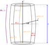 |
Fig. 1. Equilibrium configuration of the straight expanding two-layered magnetic flux tube in the presence of a background flow. |
Here l is a constant determining the thickness of the transitional layer sandwiched between the loops’s interior and exterior. It is assumed that ρ(t, r, z) is a continuous function, and ρt(t, r, z) is a monotonically decreasing function of r. The reason why the tube is split into core and transitional layers is because we want to take into account damping due to resonance absorption. The time-independent non-twisted equilibrium magnetic field is B = (Br(r, z),0, Bz(r, z)). Therefore, the divergence-free condition ∇ ⋅ B = 0 for the magnetic field can be written as
It follows from this equation that B can be expressed in terms of the magnetic flux function ψ as
In addition, we assume that the boundaries of the transitional layer are magnetic surfaces. Therefore, equations r = R(z)(1 − l/2) and r = R(z)(1 + l/2) can be written as ψ = ψi = const and ψ = ψe = const, respectively, where indices i and e refer to internal and external values. In what follows we use the cold plasma approximation and the thin tube thin boundary (TTTB) approximation. Therefore, it follows from the equilibrium configuration that the magnetic field must be potential. We have ∇ × B = 0 as a result, which can be rewritten in polar coordinates as

Substituting Eqs. (3) into (4), we express the latter equation in terms of magnetic flux function ψ as
There is also a time-dependent background flow U = (Ur(t, r, z),0, Uz(t, r, z)) present. It is assumed that the background flow velocity is parallel to the equilibrium magnetic field, U ∥ B. The plasma density and velocity are related by the mass conservation equation
The perturbations of the magnetic field and plasma velocity, b = (br, bϕ, bz) and U = (ur, uϕ, uz), are described by the linearised MHD equations in the cold plasma approximation,

where μ0 is the magnetic permeability of free space.
3. Derivation of governing equation
We first introduce the plasma displacement ξ = x − x0, where x(t, a) is the trajectory of the plasma element and a is the initial position. The components perpendicular to magnetic field lines of the displacement and velocity are given by

We assume that Bz > 0. Then, since the magnetic flux tube is thin, we can approximate ψ by its first terms of a Taylor’s expansion. In addition, we consider the tube axis as the magnetic field line ψ = const. at r = 0. Therefore, without loss of generality, we assume that ψ = 0 at r = 0, and we have from Eq. (3) that

Ruderman et al. (2017) showed that
It is easy to see that the analysis of Ruderman et al. (2017) is still valid up to Eq. (57) therein. Thus, we use Eqs. (53)–(57) of Ruderman et al. (2017) and take perturbations proportional to  , where
  is the azimuthal wavenumber, to obtain

![$$ \begin{aligned} \frac{\partial {\tilde{u_\phi }}}{\partial {T}} + \frac{U_z}{r} \frac{\partial {r \tilde{u}_\phi }}{\partial {Z}} = \frac{B_z}{\upmu _0 \rho r} \frac{\partial }{\partial {Z}} \bigg [r^2 B_z \frac{\partial }{\partial {Z}}\bigg (\frac{\xi _\phi }{r} \bigg ) \bigg ] - \frac{i \tilde{m} B^2 Q}{\rho r}. \end{aligned} $$](/articles/aa/full_html/2021/05/aa40314-21/aa40314-21-eq19.gif)
Now, eliminating ξϕ,  , and
, and  , and only keeping the leading terms with respect to ϵ, the system of equations with the respect to Q and w transforms to
where W = rw = Brξ⊥. Then, since ρ, B, and U are quantities that are independent of r and thus of ψ, employing Eq. (11) we obtain
![$$ \begin{aligned} Q = \frac{2 \psi }{\tilde{m}^2 h} \frac{\partial }{\partial {\psi }} \bigg [ \frac{1}{\upmu _0} \frac{\partial ^ 2{W}}{\partial {Z}^2} - \frac{\rho }{h^2} \bigg ( \frac{\partial }{\partial {T}} + h U \frac{\partial }{\partial {Z}} \frac{1}{h} \bigg ) \bigg ( \frac{\partial {W}}{\partial {T}} + U \frac{\partial {W}}{\partial {Z}}\bigg ) \bigg ], \end{aligned} $$](/articles/aa/full_html/2021/05/aa40314-21/aa40314-21-eq24.gif)

After differentiating Eq. (21) with respect to ψ and employing Eq. (20), we have
The solutions to Eq. (22) must decay as ψ → ∞ and be regular at ψ = 0. Therefore, as a result we have
where Qi and Qe are arbitrary functions. The internal and external boundaries are respectively defined by the equations ψ = ψi and ψ = ψe, where ψi and ψe are constants. Next, it follows from Eqs. (11) and (12) that
It follows from Eqs. (21) and (23) that in the core layer of the magnetic flux tube  , where
  is an arbitrary function. Now, we substitute Eq. (23) in Eq. (21) to obtain

where Wi and We are calculated at ψ = ψi and ψ = ψe, respectively. We now introduce the new variable

In the case  , we note that ξ⊥ is independent of r; therefore, the magnetic flux tube oscillates as a solid. In addition, Eqs. (25) and (26) reduce to the ones obtained by Ruderman et al. (2017). We now introduce jumps to this new variable and the magnetic pressure perturbation across the transitional layer:

We have the estimates  ,
,  . Then, employing Eq. (23) we obtain
![$$ \begin{aligned}&W_{\rm i} = C(1 - l/2)\eta , \quad W_{\rm e} = C[(1 + l/2)\eta + \delta \eta ] , \vspace{2mm} \nonumber \\&\displaystyle \psi _{\rm i}^{\tilde{m}/2}h^3 Q_{\rm i} = \frac{\epsilon ^{-2}C}{R^2}P\big |_{\psi =\psi _{\rm i}}, \quad \psi _{\rm e}^{-\tilde{m}/2}h^3 Q_{\rm e} = \frac{\epsilon ^{-2}C}{R^2}P\big |_{\psi =\psi _{\rm e}}. \end{aligned} $$](/articles/aa/full_html/2021/05/aa40314-21/aa40314-21-eq38.gif)
Now, let us multiply Eq. (25) by ρi, Eq. (26) by ρe, add the results, using Eqs. (12), (28), and (29), and return to the original non-scaled independent variables, yielding
with
For 0 ≤ ψ ≤ ψi we have
whereas for ψ ≥ ψe we have

where  , ηi = η(ψi), and ηe = η(ψe). Equations (30)–(33) govern oscillations of the magnetic flux tube for
  in the absence of a transitional layer (i.e. l = 0). This system is valid both for standing waves and propagating waves. In the case l ≠ 0 the system is not closed, and the jumps across the transitional layer δη and δP should be determined to close the governing system. We should also note that, in the case
  , Eq. (32) is fulfilled identically since η is independent of the r-component. In this case the above system of governing equation coincides with that obtained by Ruderman et al. (2017); the detailed investigation carried out is available in Shukhobodskiy & Ruderman (2018), Shukhobodskiy et al. (2018), Ruderman et al. (2019), and Ruderman & Petrukhin (2019), among others.
3.1. Fluting modes in the absence of transitional layer
We assume that the magnetic tube has a sharp boundary, meaning that l = 0. Since the transitional layer is absent in this equilibrium, we use Eq. (30) with the right-hand side equal to 0. Hence, we rewrite Eq. (30) as
Using Eq. (32), we reduce it to
These equations are governing for fluting oscillations and contain general information regarding the system in the absence of transitional layer. Now we employ these equations in order to facilitate the analysis.
3.2. Eigenvalue problem in the presence of stationary flow: General analysis
In this section we assume that the density and flow velocity are both independent of time and that the external plasma is at rest (i.e. Ue = 0). Since we assume that the characteristic scale of variation of the equilibrium quantities in the radial direction is the same as in the axial direction, we can neglect their radial variation inside the tube in the thin tube approximation. Then, it follows from the mass conservation in Eq. (6) that the density and flow speed are related by
where we have dropped the subscript ‘i’ for the internal flow speed U. It follows from the magnetic flux conservation that

Below, we consider standing waves and assume that the magnetic flux tube ends are fixed at the dense photosphere. Thus, we impose the boundary conditions

where L is the tube length. We look for stationary solutions, so we take η ∝ e−iωt. Then, Eq. (36) reduces to
This equation, with the boundary conditions Eq. (39), constitute an eigenvalue problem. Here we now study the general properties of this problem. We are interested in the conditions for which the tube will be stable with respect to long flute perturbations. Thus, we assume that μ0ρiU2 < 2B2, that is  , and this condition is satisfied for all z ∈ [ − L/2, L/2]. Then, we make the variable substitution
Now, multiplying the obtained equation by R4, we rewrite Eq. (40) as
![$$ \begin{aligned} \frac{\mathrm{d}}{\mathrm{d}z}\left[R^4\left(\frac{B^2}{\upmu _0} - \rho _{\rm i} U^2\right)\frac{\mathrm{d}q}{\mathrm{d}z}\right] + \omega ^2 W(z)q = 0, \end{aligned} $$](/articles/aa/full_html/2021/05/aa40314-21/aa40314-21-eq55.gif)
where
Equation (42) with the boundary conditions Eq. (39) constitute the classical Sturm-Liouville problem with the eigenvalue ω2. It follows from the general theory of the Sturm-Liouville problem (e.g. Coddington & Levinson 1955) that the eigenvalues are real and constitute a monotonically increasing unbounded sequence. The first eigenvalue is the square of the fundamental frequency, and the corresponding eigenfunction has no nodes in ( − L/2, L/2). All other eigenvalues are the squares of frequencies of corresponding overtones. The eigenfunction corresponding to the nth overtone has n − 1 nodes in ( − L/2, L/2).
It is clear that we can always take q to be real. Multiplying Eq. (42) by q, integrating the obtained equation, and using Eq. (43) we obtain
Since W(z) > 0, it follows from this equation that ω2 > 0, meaning that all the eigenfrequencies are real. This also implies that the inequality  is a sufficient condition for stability inside the tube with respect to long flute perturbations. To obtain an equation describing the boundary, we follow the analysis of Ruderman et al. (2017) to determine whether the stability condition on the boundary is different, with a sufficient condition
  . We note that this condition is sufficient but not necessary. On the other hand, this analysis does not prove that the tube is stable if the condition
  is satisfied. While it guaranties that the tube is stable with respect to long flute perturbations, it can be unstable with respect to other types of perturbations.
4. Flute oscillations of magnetic flux tube with slowly varying density
Below, we now consider flute oscillations of a magnetic flux tube with slowly varying density. We assume that the magnetic flux tube is fixed at the dense photosphere, which means that the boundary condition in Eq. (40) is satisfied. In addition, we also assume that the characteristic time of density variation, tch, is much greater than the characteristic time of oscillations. We note that this is not a very restrictive assumption.
4.1. Derivation of adiabatic invariant
We denote the ratio of tch to the characteristic time of oscillations as ν−1, where ν ≪ 1. Hence, the characteristic time of oscillations is νtch. On the other hand, it is also of the order of the loop length divided by the characteristic flute speed, which is equal to  , where ρch is the characteristic density. We have, as a result,
Following this estimate, let us now introduce the scaled magnetic field  . Then, we rewrite Eqs. (33) and (42) as
Now, we use the Wentzel-Kramer-Brillouin (WKB) method (e.g. Bender & Orszag 1978) and look for solution to this equation in the form
![$$ \begin{aligned} \eta = S(t,r,z) \exp [\nu ^{-1} \Theta (t)]. \end{aligned} $$](/articles/aa/full_html/2021/05/aa40314-21/aa40314-21-eq66.gif)
Then, we expand S in the series
We substitute Eq. (48) in Eqs. (46) and (47), using Eq. (49), and collecting terms of order ν−2 we obtain
and
where
Inside the magnetic flux tube  and outside the flux tube
  , hence adding Eqs. (50) and (51), we obtain
where
Since we assume that the magnetic flux tube is fixed in the dense photosphere (i.e. there is line-tying) we now have that

Therefore, Eqs. (53) and (55) constitute the classical Sturm-Liouville problem as a result. An approximation of such order is called the approximation of geometrical optics (e.g. Bender & Orszag 1978). The Sturm-Liouville problem of Eqs. (53) and (55) coincide with a problem obtained by Dymova & Ruderman (2005) to describe oscillations of magnetic flux tubes whose density varies along the tube, and by Ruderman et al. (2008) to describe kink oscillation of magnetic tubes whose density and cross-section radius vary along the tube.
Below, we assume that Ω2 is an eigenvalue and S0 the corresponding eigenfunction. In accordance with the general theory (e.g. Coddington & Levinson 1955), Ω2 is real. It is easy to prove that Ω2 > 0 by multiplying Eq. (53) by S0, then integrating by parts with respect to z from −L/2 to L/2 and using the boundary condition (55). We can always assume that S0 is a real function.
Now, we collect terms of the order ν−1 to obtain
and
where

and

Taking into account that inside the magnetic flux tube  and outside the flux tube
  , from Eqs. (56) and (57), we have
This order of approximation is the approximation of the physical optics. S1 must satisfy the boundary conditions
The homogeneous counterparts of the boundary value problem constituted by Eqs. (53) and (60), and the boundary condition Eqs. (55) and (61) have the non-trivial solution S1 = S0. This implies that the boundary value problem determining S1 has a solution only if the right-hand side of Eq. (60) satisfies the compatibility condition, which is the condition that it should be orthogonal to S0. To obtain this condition we multiply Eq. (60) by S0, then integrate with respect to z from −L/2 to L/2. After some algebra we obtain that
Using integration by parts, and some algebra, we eventually obtain
where
The left-hand side of Eq. (63) is an adiabatic invariant. Equation (63) states that this invariant is conserved. It is easy to see that the derivation for adiabatic invariant and approximations of the 0th order on the boundary presented by Ruderman et al. (2017) are still valid. It is also worth noting that the adiabatic invariant is the same as that obtained by Ruderman (2011a) for oscillations of magnetic tubes with constant cross-section radius. Hence, the tube expansion only affects the temporal evolution of flute oscillations of magnetic flux tubes with varying density through Ck, VAi, VAe, and S0 that all depend on R(z).
4.2. Effect of cooling on flute oscillations of coronal magnetic loops
The main cause of cooling of a coronal loop is radiation. The intensity is proportional to the plasma density squared for optically think plasmas. The energy deposition that can cover the losses of energy in the rarefied external plasma could be too small to cover the energy loss in the internal region of a magnetic flux tube. Therefore, we can assume that the plasma temperature remains constant outside the magnetic flux tube. As was found in Aschwanden & Nightingale (2005), and Morton & Erdélyi (2010), the temperature evolution inside the loop is approximated by exponentially decaying function,

where we assume that, at the initial time t = 0, the cooling begins. In addition, we assume that the plasma temperature is the same at this initial time in the external and internal regions, so that the temperature of the external plasma remains equal to T0. In what follows we consider a magnetic flux tube that has a semi-circular shape. We neglect the effect of flux tube curvature on fluting oscillations. The shape of the loop determines the density variation along the loop only as a result, t. The density of the external plasma is given by the barometric formula
where ρf is the plasma density at the footpoints inside the magnetic flux tube, which is assumed to be constant, and ζ is the ratio of internal to external plasma densities at initial time,

kB is the Boltzmann constant, g is the gravity acceleration, and m is the mean mass per particle equal to one-half of the proton mass for a proton-electron plasma. The flow inside the magnetic flux tube is caused by plasma cooling.
It is easy to show that the analysis of Ruderman (2011b) still holds true even for fluting modes described in the model presented in this manuscript. Thus, the effect of the flow on the plasma density is fairly weak for the typical coronal conditions and the observed cooling times. Therefore, the barometric formula provides a sufficiently good approximation of the plasma density in the internal region of the magnetic flux tube. We have
where
Since the background magnetic field is straight and not twisted, we can describe the variation of cross-section radius of the tube with the same expression as in Ruderman et al. (2008),
where Rf is the cross-section radius of the magnetic flux tube at the footpoints, lc is an arbitrary positive constant with the dimension of length, and λ = R(0)/Rf. Ruderman et al. (2008) showed that for the z-component of the magnetic field to be positive everywhere in the region |z|≤L/2, the expansion factor must satisfy the inequality λ < λm, where
Here λm is a monotonically increasing function of L/lc, such that λm → 1 as L/lc → 0, and λm → 1.87 as L/lc → ∞. Since the expansion of coronal loop factor does not exceed 1.5, the careful choice of the ration L/lc allows us to cover the entire range of the expansion factor variation.
Now, we introduce the following dimensionless variables and parameters
where the kink speed at the footpoints is
Therefore, we can reduce Eq. (53) to
![$$ \begin{aligned} \frac{\partial ^ 2{S_0}}{\partial {Z}^2}&+ \frac{\varpi ^2 \Lambda ^4(Z) S_0}{4 (\zeta +1)} \nonumber \\&\times [\zeta \exp (-\kappa e^{\tau } \cos (\pi Z/2) + \exp (- \kappa \cos (\pi Z/2)]=0. \end{aligned} $$](/articles/aa/full_html/2021/05/aa40314-21/aa40314-21-eq96.gif)
We have dropped the prime in Eq. (74). We should also note that in order to obtain solutions for the plasma displacement in the internal region and in the external region, which both depend on radial component, we first need to find a solution for the plasma displacement at the boundary of Eq. (74). We also know that W = rR(z)Bη, implying that inside the tube  and in the external region, in the vicinity of the magnetic flux tube,
  , where
  is an arbitrary function. Therefore we obtain
The eigenfunction S0 is accurately determined up to the multiplication of the arbitrary function of τ, and the dependence on ψ is determined by Eq. (75). We can always fix its value to one particular point. We assume X(τ, Z) to be an eigenfunction corresponding to the fundamental mode, which satisfies the condition X(τ, 0) = 1. Then, the general solution to the eigenvalue problem of the fundamental mode is S0(τ, Z, ψ) = A(τ, ψ)X(τ, Z), where A(τ, ψ) is the oscillation amplitude at Z = 0. With the aid of Eq. (75) we derive
where
Therefore, we rewrite Eq. (63) as
![$$ \begin{aligned} \varpi A^2(\tau , \psi ) \int ^{1}_{-1}&X^2 \Lambda ^4 [ \zeta \exp ( - \kappa e^{\tau } \cos (\pi Z/2)) \nonumber \\&+ \exp (- \kappa \cos (\pi Z/2))] \mathrm{d}Z = \text{ const}. \end{aligned} $$](/articles/aa/full_html/2021/05/aa40314-21/aa40314-21-eq105.gif)
We also note that
Then, we set lc = 4 so that the entire observed range of possible λ is covered by the expansion model and solve Eqs. (80)–(82) numerically to obtain the dependence of dimensionless amplitude on r for various values of  .
.
First, we note that it follows from Fig. 2 that the higher the value of λ, the lower the amplitude closer to the magnetic flux tube core. The phenomenon that can be spotted is that the amplitude increases between the initial and final time. Furthermore, the higher the expansion factor, the higher the final amplitude, which is consistent with the result obtained by Shukhobodskiy et al. (2018). The other pattern to be noted in Fig. 2 is that when the value of  is higher, more oscillations are localised at the tube boundary. This latter conclusion is in agreement with Soler (2017). Furthermore, we note that the expansion factor λ of the magnetic flux tube is of paramount importance in determining the oscillation intensity. This can be especially observed in the bottom panels of Fig. 2, where oscillations occur close to the tube boundary magnetic field lines to such an extent, that even the region above the boundary in the footpoints would not oscillate at the apex of the tube for even a mildly expanding flux tube.
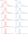 |
Fig. 2. Dependence of dimensionless amplitude on r/Rf. Left panels: amplitude variation at the initial time τ = 0, and right panels: amplitude variation at the final time τ = 1. The solid, dash-dotted, and dot-dashed lines correspond to λ = 1, 1.1, and (1.3, 1.5), respectively. From top to bottom, the panels correspond to |

It follows from Fig. 3 that ζ has no effect on the initial amplitude variation in the distance from the core region. On the other hand, at the final time τ = 1 it is possible to observe three separate phenomena. First of all, increasing the wave number  localises the oscillation closer to the boundary. Secondly, when the value of ζ increases, the amplification of oscillations due to cooling become stronger. Finally, the increase in
  leads to a reduction in the spread between the oscillation variation across the tube for different values of ζ, preserving the trend that the higher the value of ζ, the higher the amplification due to cooling.
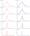 |
Fig. 3. Dependence of dimensionless amplitude on r/Rf. Left panels: amplitude variation at the initial time τ = 0, and right panels: amplitude variation at final time τ = 1. The solid, dash-dotted, and dot-dashed lines correspond to ζ = 1, 2, and (3, 4), respectively. From top to bottom, the panels correspond to |

Figure 4 represents the evolution of oscillation of magnetic flux tube both through time and distance from the annulus. We find, for both the top and bottom panels, that the amplitude increases with time. Furthermore, higher values of  lead to the localisation of oscillation closer to the boundary. On the other hand, an increasing expansion factor λ not only leads to an increase in the oscillation amplitude, but also shifts the localisation of oscillation of the magnetic flux tube further from the centre. Therefore we conclude that not only does
  have an important role in the evolution of the cooling system, but also variations in the expansion λ and density ratio ζ, with the latter having a significant deviation between the initial and final times.
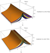 |
Fig. 4. Dependence of dimensionless amplitude on r/Rf and time τ for ζ = 3. The orange, purple, yellow, and dark purple colour schemes respectively correspond to |


We also note that the above analysis is valid for any cooling function T(t). For example, if we take

where

the loop is first cooled and then heated. The parameter α in Eq. (84) is responsible for the strength of cooling and heating in such temperature distributions. Therefore, as a result, it is possible to rewrite Eqs. (74) and (80) as
![$$ \begin{aligned}&\frac{\partial ^ 2{S_0}}{\partial {Z}^2} + \frac{\varpi ^2 \Lambda ^4(Z) S_0}{4 (\zeta +1)}[\zeta \exp (-\kappa (1- \alpha \sin (\tau \pi ))^{-1} \cos (\pi Z/2)) \nonumber \\&\quad +\exp (- \kappa \cos (\pi Z/2))]=0 \end{aligned} $$](/articles/aa/full_html/2021/05/aa40314-21/aa40314-21-eq120.gif)
and
![$$ \begin{aligned} \varpi A^2(\tau , \psi ) \int ^{1}_{-1}&X^2 \Lambda ^4 [ \zeta \exp ( - \kappa (1- \alpha \sin (\tau \pi ))^{-1} \cos (\pi Z/2)) \nonumber \\&+ \exp (- \kappa \cos (\pi Z/2))] \mathrm{d}Z = \text{ const}. \end{aligned} $$](/articles/aa/full_html/2021/05/aa40314-21/aa40314-21-eq121.gif)
We take, for example, α = 0.9 and solve the Eqs. (85) and (86) numerically. It follows from Fig. 5 that during the initial cooling the amplitude increases, whereas as heating starts the oscillation experiences damping through time. Nevertheless, the pattern with respect to other variables is similar to that of the initial case with exponential cooling.
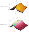 |
Fig. 5. Dependence of dimensionless amplitude on r/Rf and time τ for ζ = 3. The orange, purple, green, and pink colour schemes respectively correspond to |


5. Conclusion
In this article we studied the oscillations of fluting modes for an expanding magnetic flux tube in the presence of a bulk flow. The plasma density and the velocity vary both in space and with time. However, we assume that the characteristic scale of variation of these quantities along the loop and across the loop are of the same order and may vary in a thin transitional layer. Starting from the linearised MHD equations and with the aid of multi-scale expansion, we derived Eqs. (29)–(34), which govern the flute oscillations of a magnetic flux tube, both for standing and propagating waves. This system is closed in the absence of a transitional layer. However, when the transitional layer is present additional information is needed to solve the governing equations since jumps in pressure and displacement may manifest within the system. In order to close this system, these jumps should be expressed in terms of the displacement.
The derived set of equations is then used to study the effect of density variation with time on oscillations for a magnetic flux tube. We assumed that the characteristic time of the density variation is much greater than the characteristic time of the oscillation. Via the WKB method, we were able to derive an adiabatic invariant (the quantity conserved while plasma density evolves).
Furthermore, by considering cooling of a curved magnetic flux tube with ends fixed to dense photosphere (i.e. imposing line-tying) we numerically solved the system of governing equations. First of all, we found that for all values of m the oscillation amplitude increases with time. The same conclusion was made previously by Ruderman et al. (2017) for kink modes. Moreover, the higher the value of m is, the closer the oscillation is to the boundary, where this effect becomes less prominent as time passes; this is a similar conclusion to that recorded previously (e.g. Soler 2017).
We also found that the expansion factor not only shifts the oscillation localisation toward higher values, but also modifies the oscillation variation pattern.
Another fascinating phenomenon found is that the higher the density ratio is between the external and internal plasma, the stronger the amplification is for all values of m. As a result, higher density contrast results in stronger oscillation. Furthermore, although the higher the value of m is, the more localised it is towards the boundary of the oscillation; nevertheless, the increase in values of the density ratio ζ allows some compensation of these events by shifting the oscillation from the boundary. This effect adds additional knowledge to the previous understanding of flute oscillation, which suggested that oscillation is concentrated at the boundary of the object.
Last but not least, we note that a correct combination of a magnetic flux tube expansion and the ratio of internal to external density could negate the effect of increase due to higher azimuthal wavenumber, thus making it possible for high m flute modes not only to present properties of surface waves, but also body waves.
Flute modes in coronal loops have not yet been detected with the currently available observational suits. However, detecting these modes in the presence of cooling, high magnetic flux tube expansion, and loops with denser regions will be more likely in future observations thanks to the increased amplitude over time. This will allow us to limit the number of objects of interest, where better instruments should be used in order to have a higher chance of discovering flute oscillations.
Acknowledgments
The authors are grateful to M.S. Ruderman for a number of useful comments and for proofreading the article. D.S. is grateful to the University of Sheffield for the support received. A.A.Sh is thankful to Interreg Northwest Europe for the support received to conduct this research through grant number: NWE847. RE is grateful to STFC (UK, grant number ST/M000826/1). RE also acknowledges support from the Chinese Academy of Sciences President’s International Fellowship Initiative (PIFI, grant number 2019VMA0052) and The Royal Society (grant nr IE161153).
References
- Andries, J., van Doorsselaere, T., Roberts, B., et al. 2009, Space Sci. Rev., 149, 3 [NASA ADS] [CrossRef] [Google Scholar]
- Antolin, P., Yokoyama, T., & Van Doorsselaere, T. 2014, ApJ, 787, L22 [NASA ADS] [CrossRef] [Google Scholar]
- Aschwanden, M. J., & Nightingale, R. W. 2005, ApJ, 633, 499 [NASA ADS] [CrossRef] [Google Scholar]
- Banerjee, D., Erdélyi, R., Oliver, R., & O’Shea, E. 2007, Sol. Phys., 246, 3 [NASA ADS] [CrossRef] [Google Scholar]
- Bender, C. M., & Orszag, S. A. 1978, Advanced Mathematical Methods for Scientists and Engineers (New York: McGraw-Hill) [Google Scholar]
- Coddington, E. A., & Levinson, N. 1955, Theory of Ordinary Differential Equations (New York: McGraw-Hill) [Google Scholar]
- Dymova, M. V., & Ruderman, M. S. 2005, Sol. Phys., 229, 79 [NASA ADS] [CrossRef] [Google Scholar]
- Edwin, P. M., & Roberts, B. 1983, Sol. Phys., 88, 179 [Google Scholar]
- Erdélyi, R. 2006a, R. Soc. London Philos. Trans. Ser. A, 364, 351 [Google Scholar]
- Erdélyi, R. 2006b, in Proceedings of SOHO 18/GONG 2006/HELAS I, Beyond the spherical Sun, eds. K. Fletcher, & M. Thompson, ESA SP-624 [Google Scholar]
- Erdélyi, R., & Morton, R. J. 2009, A&A, 494, 295 [NASA ADS] [CrossRef] [EDP Sciences] [Google Scholar]
- Erdélyi, R., & Taroyan, Y. 2008, A&A, 489, L49 [NASA ADS] [CrossRef] [EDP Sciences] [Google Scholar]
- Kuridze, D., Mathioudakis, M., Morgan, H., et al. 2019, ApJ, 874, 126 [NASA ADS] [CrossRef] [Google Scholar]
- Magyar, N., & Van Doorsselaere, T. 2016, A&A, 595, A81 [NASA ADS] [CrossRef] [EDP Sciences] [Google Scholar]
- Morton, R. J., & Erdélyi, R. 2010, A&A, 519, A43 [NASA ADS] [CrossRef] [EDP Sciences] [Google Scholar]
- Nakariakov, V. M., & Ofman, L. 2001, A&A, 372, L53 [NASA ADS] [CrossRef] [EDP Sciences] [Google Scholar]
- Nakariakov, V. M., & Verwichte, E. 2005, Liv. Rev. Sol. Phys., 2, 3 [Google Scholar]
- Nakariakov, V. M., Pilipenko, V., Heilig, B., et al. 2016, Space Sci. Rev., 200, 75 [Google Scholar]
- Nelson, C. J., Shukhobodskiy, A. A., Erdélyi, R., & Mathioudakis, M. 2019, Front. Astron. Space Sci., 6, 45 [Google Scholar]
- Pascoe, D. J., Goddard, C. R., Nisticò, G., Anfinogentov, S., & Nakariakov, V. M. 2016, A&A, 585, L6 [NASA ADS] [CrossRef] [EDP Sciences] [Google Scholar]
- Pascoe, D. J., Russell, A. J. B., Anfinogentov, S. A., et al. 2017, A&A, 607, A8 [NASA ADS] [CrossRef] [EDP Sciences] [Google Scholar]
- Ruderman, M. S. 2003, A&A, 409, 287 [NASA ADS] [CrossRef] [EDP Sciences] [Google Scholar]
- Ruderman, M. S. 2011a, Sol. Phys., 271, 55 [NASA ADS] [CrossRef] [Google Scholar]
- Ruderman, M. S. 2011b, Sol. Phys., 271, 41 [NASA ADS] [CrossRef] [Google Scholar]
- Ruderman, M. S. 2017, Sol. Phys., 292, 111 [Google Scholar]
- Ruderman, M. S., & Erdélyi, R. 2009, Space Sci. Rev., 149, 199 [NASA ADS] [CrossRef] [Google Scholar]
- Ruderman, M. S., & Petrukhin, N. S. 2019, A&A, 631, A31 [EDP Sciences] [Google Scholar]
- Ruderman, M. S., Verth, G., & Erdélyi, R. 2008, ApJ, 686, 694 [NASA ADS] [CrossRef] [Google Scholar]
- Ruderman, M. S., Goossens, M., & Andries, J. 2010, Phys. Plasmas, 17, 082108 [NASA ADS] [CrossRef] [Google Scholar]
- Ruderman, M. S., Shukhobodskiy, A. A., & Erdélyi, R. 2017, A&A, 602, A50 [NASA ADS] [CrossRef] [EDP Sciences] [Google Scholar]
- Ruderman, M. S., Shukhobodskaya, D., & Shukhobodskiy, A. A. 2019, Front. Astron. Space Sci., 6, 10 [Google Scholar]
- Ryutov, D. D., & Ryutova, M. P. 1976, Sov. Phys. - JETP, 43, 491 [Google Scholar]
- Shukhobodskiy, A. A., & Ruderman, M. S. 2018, A&A, 615, A156 [NASA ADS] [CrossRef] [EDP Sciences] [Google Scholar]
- Shukhobodskiy, A. A., Ruderman, M. S., & Erdélyi, R. 2018, A&A, 619, A173 [EDP Sciences] [Google Scholar]
- Shukhobodskaia, D., Shukhobodskiy, A. A., Nelson, C. J., Ruderman, M. S., & Erdélyi, R. 2021, Front. Astron. Space Sci., 7, 579585 [Google Scholar]
- Soler, R. 2017, ApJ, 850, 114 [NASA ADS] [CrossRef] [Google Scholar]
- Terradas, J., Andries, J., Goossens, M., et al. 2008, ApJ, 687, L115 [Google Scholar]
- Terradas, J., Magyar, N., & Van Doorsselaere, T. 2018, ApJ, 853, 35 [NASA ADS] [CrossRef] [Google Scholar]
- Tomczyk, S., McIntosh, S. W., Keil, S. L., et al. 2007, Science, 317, 1192 [Google Scholar]
All Figures
|
Fig. 1. Equilibrium configuration of the straight expanding two-layered magnetic flux tube in the presence of a background flow. |
| In the text | |
|
Fig. 2. Dependence of dimensionless amplitude on r/Rf. Left panels: amplitude variation at the initial time τ = 0, and right panels: amplitude variation at the final time τ = 1. The solid, dash-dotted, and dot-dashed lines correspond to λ = 1, 1.1, and (1.3, 1.5), respectively. From top to bottom, the panels correspond to |
| In the text | |
|
Fig. 3. Dependence of dimensionless amplitude on r/Rf. Left panels: amplitude variation at the initial time τ = 0, and right panels: amplitude variation at final time τ = 1. The solid, dash-dotted, and dot-dashed lines correspond to ζ = 1, 2, and (3, 4), respectively. From top to bottom, the panels correspond to |
| In the text | |
|
Fig. 4. Dependence of dimensionless amplitude on r/Rf and time τ for ζ = 3. The orange, purple, yellow, and dark purple colour schemes respectively correspond to |
| In the text | |
|
Fig. 5. Dependence of dimensionless amplitude on r/Rf and time τ for ζ = 3. The orange, purple, green, and pink colour schemes respectively correspond to |
| In the text | |
Current usage metrics show cumulative count of Article Views (full-text article views including HTML views, PDF and ePub downloads, according to the available data) and Abstracts Views on Vision4Press platform.
Data correspond to usage on the plateform after 2015. The current usage metrics is available 48-96 hours after online publication and is updated daily on week days.
Initial download of the metrics may take a while.