| Issue |
A&A
Volume 649, May 2021
|
|
|---|---|---|
| Article Number | A123 | |
| Number of page(s) | 15 | |
| Section | The Sun and the Heliosphere | |
| DOI | https://doi.org/10.1051/0004-6361/202040199 | |
| Published online | 26 May 2021 | |
On the (in)stability of sunspots⋆,⋆⋆
1
Leibniz-Institut für Sonnenphysik, Schöneckstr. 6, 79104 Freiburg, Germany
e-mail: This email address is being protected from spambots. You need JavaScript enabled to view it.
2
High Altitude Observatory, NCAR, PO Box 3000, Boulder, CO 80307, USA
Received:
21
December
2020
Accepted:
4
March
2021
Abstract
Context. The stability of sunspots is one of the long-standing unsolved puzzles in the field of solar magnetism and the solar cycle. The thermal and magnetic structure of the sunspot beneath the solar surface is not accessible through observations, thus processes in these regions that contribute to the decay of sunspots can only be studied through theoretical and numerical studies.
Aims. We study the effects that destabilise and stabilise the flux tube of a simulated sunspot in the upper convection zone. The depth-varying effects of fluting instability, buoyancy forces, and timescales on the flux tube are analysed.
Methods. We analysed a numerical simulation of a sunspot calculated with the MURaM code. The simulation domain has a lateral extension of more than 98 Mm × 98 Mm and extends almost 18 Mm below the solar surface. The analysed data set of 30 hours shows a stable sunspot at the solar surface. We studied the evolution of the flux tube at defined horizontal layers (1) by means of the relative change in perimeter and area, that is, its compactness; and (2) with a linear stability analysis.
Results. The simulation shows a corrugation along the perimeter of the flux tube (sunspot) that proceeds fastest at a depth of about 8 Mm below the solar surface. Towards the surface and towards deeper layers, the decrease in compactness is damped. From the stability analysis, we find that above a depth of 2 Mm, the sunspot is stabilised by buoyancy forces. The spot is least stable at a depth of about 3 Mm because of the fluting instability. In deeper layers, the flux tube is marginally unstable. The stability of the sunspot at the surface affects the behaviour of the field lines in deeper layers by magnetic tension. Therefore the fluting instability is damped at depths of about 3 Mm, and the decrease in compactness is strongest at a depth of about 8 Mm. The more vertical orientation of the magnetic field and the longer convective timescale lead to slower evolution of the corrugation process in layers deeper than 10 Mm.
Conclusions. The formation of large intrusions of field-free plasma below the surface destabilises the flux tube of the sunspot. This process is not visible at the surface, where the sunspot is stabilised by buoyancy forces. The onset of sunspot decay occurs in deeper layers, while the sunspot still appears stable in the photosphere. The intrusions eventually lead to the disruption and decay of the sunspot.
Key words: Sun: magnetic fields / sunspots / instabilities
The animation is available at https://www.aanda.org
This paper is mainly based on Part I of the Ph.D. thesis “On the decay of sunspots”, https://freidok.uni-freiburg.de/data/165760
© H. Strecker et al. 2021
 Open Access article, published by EDP Sciences, under the terms of the Creative Commons Attribution License (https://creativecommons.org/licenses/by/4.0), which permits unrestricted use, distribution, and reproduction in any medium, provided the original work is properly cited.
1. Introduction
The lifetime of sunspots covers a broad range of a few days to a few months (Martínez Pillet 2002; van Driel-Gesztelyi & Green 2015). The observational evolution and decay process of sunspots distinguishes a photometric and a magnetic decay (Martínez Pillet 2002). The origin of the differences in lifetime and the flux removal is still not completely understood. In addition, the onset of the decay process is not clear. In some cases, a sunspot already starts to decay, that is, loose magnetic flux, while it might at the same time gain magnetic flux by coalescence (Solanki 2003). This means that the process that leads to the decay of a sunspot operates already before the sunspot has fully developed (McIntosh 1981). The opaqueness of the photosphere inhibits direct observations of processes below the solar surface. This limits our ability of fully understanding sunspot evolution from direct observations. Numerical models are used to obtain a more complete image of sunspots. A variety of different models, especially static ones, has been presented over the years (for an overview of different (static) sunspot models, we refer to Jahn (1997). The basic assumption for a magnetohydrostatic model is that the sunspot is a monolithic, single magnetic flux tube in and below the photosphere (Schlüter & Temesváry 1958). For a better agreement of the modelled sunspots with observations, Simon & Weiss (1970) implemented a current sheet at the boundary of the flux tube. This current sheet, also called magnetopause, balances the internal pressure with the pressure in the surroundings. The discontinuity of the pressure across the current sheet is correlated to a jump in the field strength (Jahn 1992; Jahn & Schmidt 1994).
To study the stability of sunspots in the convection zone, Meyer et al. (1977) adapted a magnetohydrostatic model. They embedded a flux tube with an axisymmetric meridional field (Br, 0, Bz) in the non-magnetised plasma of the upper convection zone. For the magnetic flux tube to be in equilibrium with the surrounding plasma, they assumed the two regions to be separated by a surface S (see Fig. 1). This surface is a current sheet that causes the abrupt drop of the magnetic field and thereby horizontally balances the pressure of the flux tube, pf, and of the surrounding plasma, pp. Meyer et al. (1977) assumed that instabilities of the surroundings, for instance, convection, do not affect the stability of this system. In addition, the plasma in the tube was stably stratified and magnetohydrodynamically stable. Then any perturbation leading to an instability depends on the equilibrium balance at the surface, S. To describe the stability, they took the decreasing pressure difference (pp − pf) with height into account. In addition, the fanning-out of the field with height, which causes a change in inclination angle, χ, of the surface S to the vertical (see Fig. 1) and a change in effect of the gravitational acceleration, g, onto the magnetised plasma. Finally, the curving of the field causes magnetic tension forces, and the criterion for stability is written as
 (1)
(1)
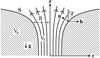 |
Fig. 1. Geometry of a magnetic flux tube (Vf) embedded in field-free plasma (Vp) (image adapted from Meyer et al. 1977). |
with Rc the radius of curvature of the surface S. For a more detailed derivation of the criterion, we refer to Meyer et al. (1977) and Strecker (2020). Based on this inequality, a magnetic flux tube in the upper layers of the convection zone has to balance two main effects to remain stable: (1) The plasma of the magnetic flux tube is less dense than the surrounding plasma, therefore the spot floats on the quiet Sun. (2) The concave curvature of the magnetic field lines has a destabilising effect and causes the tube to become vulnerable to interchange instability.
Interchange instability is a well-known process in which a cylindrical magnetic flux tube that is perturbed at its outer boundary is deformed. Bundles of field lines are transferred into the non-magnetised neighbourhood. On exchange, regions that were originally occupied by magnetic field lines are occupied by non-magnetised plasma. The individual volumes remain unchanged in this interchange process. The cylindrical flux tube obtains a rippled interface, similar to a fluted column. Therefore the process is also called fluting instability. The direction of the curving of the field lines towards the non-magnetised plasma affects the stability. If the curvature is concave, the rippled interface increases the cross-section and hence destabilises the flux tube further. A detailed explanation of interchange instability can be found in Priest (2014).
Schüssler (1984) developed the model of Meyer et al. (1977) further to study the effect of velocity fields on the instability of flux tubes. He found that converging convective flow cells surrounding the flux tube and flows along the field lines within the flux tube do not have a stabilising effect. Instead, their contribution can be destabilising. Only flows with an azimuthal component around the magnetic flux tube have the ability to stabilise. Parker (1979) made use of the stability criterion of Meyer et al. (1977). At a sufficiently large depth below the surface, field lines are able to separate from the spot through interchange instability. Parker suggested that a sunspot is not a monolithic, single flux tube below the solar surface. Instead, at about 1Mm below the photosphere, the monolithic structure divides into several smaller flux bundles. Buoyancy and convective downdrafts allow these bundles to bunch together towards the photosphere, and stabilise them against interchange processes (Parker 1979; Jahn 1992). This model is often referred to as the spaghetti or jelly fish model.
Studies performed by means of the photometric evolution of the sunspot take advantage of the change in area of the sunspot in the photosphere in time. A variety of studies have been performed, resulting in different decay processes and scenarios. A linear decay law was found by Bumba (1963) for recurrent sunspots and was found to fit the distribution in later studies. Martínez Pillet et al. (1993) proposed a parabolic decay rate, with the area being a quadratic function in time. However, they noted that it is difficult to distinguish linear or quadratic decay rates based on the observations. Petrovay & van Driel-Gesztelyi (1997) also proposed a parabolic decay law for their observed sunspots. The determination of a decay law is important to understand the decay process of the sunspots. A linear decay implies that the loss of flux occurs everywhere within the sunspot through turbulent diffusion of the magnetic field (e.g., Meyer et al. 1974; Solanki 2003). Instead, a parabolic decay law could be caused by erosion of the sunspot at its boundary, for instance, by supergranular motions (Simon & Leighton 1964) or turbulent motions on a granular-size scale (Petrovay & Moreno-Insertis 1997). These models shift the question of an area change during sunspot decay to possible scenarios regarding the loss of magnetic flux from the sunspots. A loss of magnetic flux across the whole area of the sunspot is supported by the appearance of moving magnetic features (MMFs). These appear in the non-magnetised moat region surrounding a sunspot and were first reported by Sheeley (1969). Harvey & Harvey (1973) were the first to propose that the magnetic patches pull off magnetic flux from the sunspot while moving away. However, later investigations found imbalances between the sunspot magnetic flux loss and the magnetic flux transported by MMFs (e.g., Martínez Pillet 2002; Kubo et al. 2007). Different types of MMFs were proposed to exist, and were classified according to their polarity (Shine & Title 2000). Unipolar features of both polarities are observed as well as bipolar features. Martínez Pillet (2002) proposed that only the unipolar features with the same polarity as the sunspot are related to the loss of flux from the sunspot, that is, sunspot decay. Unipolar features with opposite polarity as the sunspot and bipolar features might be extensions of penumbral filaments. Such a scenario was first proposed by Zhang (1992). Thomas et al. (2002) described such a scenario in further detail, with the bipolar features showing a sea-serpent structure. Kubo et al. (2007), Kubo (2012), and Verma et al. (2012) also found that the total magnetic flux of the MMFs is far higher than the flux loss of the sunspot. Therefore the polarity of the MMFs has to be considered to determine their relation to sunspot decay. In addition, Rempel (2015) found in simulations that the emergence and submergence of horizontal field in the moat region also contributes substantially to the flux budget of a sunspot. Specifically, these contributions tend to offset the flux transport due to MMFs. This might be an explanation for observations of MMFs in the surroundings of stable sunspots that last for several months (van Driel-Gesztelyi & Green 2015). The relation of MMFs to the decay process of sunspots is still unclear.
The knowledge that the flux tube of a sunspot evolves below the photosphere might lead to insights into the decay process. However, the models described above are static. The advent of new computers with more power and larger computational domains enabled setting up realistic magnetohydrodynamic (MHD) simulations in the past years. In this study we make use of a 3D MHD simulation of a sunspot to study the evolution of a sunspot in the upper convection zone and in the photosphere. In Sect. 2 we describe the setup and characteristics of the simulation domain that hosts the sunspot. In addition, we determine the flux tube boundary. We analyse the flux tube in Sect. 3 by studying the evolution of its structure, and by performing a linear stability analysis in Sect. 4. In both sections we describe the respective methods and results separately. The results of both studies are combined and discussed in Sect. 5. Finally, a picture of the stability of the flux tube in the upper convection zone and photosphere and a decay scenario of sunspots is presented in Sect. 6.
2. Data and methods
We analysed a sunspot in a 3D MHD simulation. It was calculated with the MURaM code by Rempel (2015). He calculated two different simulations. We used the simulation that is calculated with a modified numerical diffusivity. For a more detailed description of the calculation and the specification, we refer the reader to Sect. 2 of Rempel (2015).
The simulation domain had a size of 98.308 × 98.308 × 18.432 Mm3 and was computed on a grid with a 48 × 48 × 24 km3 cell size. The analysed data set had an increased grid cell size of 96 km in horizontal direction and a grid spacing of 48 km in vertical direction. Thus, the analysed 3D domain was composed of 1024 × 1024 grid cells horizontal and 384 grid cells vertical. The data show the sunspot with an average diameter of 30 Mm, the surrounding moat flow with an average extension of 10 Mm at the surface, and the surrounding quiet Sun. The vertical extension of the simulation domain enabled us to cover sub-photospheric regions with their own characteristics, such as convective motions. The simulation used the setup of Rempel (2012), in which a more horizontal field is imposed through the top boundary in order to create an extended penumbra.
The complete simulation covered a duration of 100 hours. In this analysis we considered a section of 30 hours. This section covers the time range from tsim = 50 h until tsim = 79.75 h, with a cadence of 15 min. For the analysis we used the 3D data of the temperature, T, pressure, p, density, ρ, the three components of the magnetic field (Bx, By, Bz), and the velocity (vx, vy, vz). In addition, 2D maps of the magnetic field strength and intensity for selected layers of constant optical depth, τ, were used.
The vertical extension of the simulation domain of 18.432 Mm covers the photosphere and uppermost part of the convection zone. The two regions are attempted to be separated by a solar surface. To define a constant layer within the gridded simulation domain and define it as the solar surface, we determined an average τ = 1 layer. To do this, the optical depth along vertical rays was calculated from the temperature and pressure of each grid cell using the tabulated Rosseland mean opacity, which was also used to advance the grey simulation in the first place. The Rosseland opacity was computed from Kurucz (1993) opacity tables. The z-layer, in the following termed solar surface, is defined as the mean z-position where τ = 1. A restriction was made by only taking into account cells outside the sunspot region, that is, the moat and quiet-Sun region. This layer was defined as z = 0 Mm. Thus, the convection zone extends down to z = −17.71 Mm with negative z-values. Regions in the photosphere have positive z-values with an extension up to 0.720 Mm above the solar surface.
In this analysis the evolution of the magnetic flux tube of the sunspot is studied from the solar surface downward through the convective region. In this region, we focus on defined depths in steps of Δz = 0.625 Mm from z = 0 Mm down to z = −15 Mm.
2.1. Convective timescale
The evolution of the flux tube of the sunspot is affected by the surrounding regions. We studied the time evolution of the flux tube at different depths in time. Therefore the changing timescales of convective motion within the convection zone had to be considered. In the following we determine the convective timescale for different depths of the simulation domain using the mixing length theory (see e.g., Stix 2002). In addition, we compare the obtained timescale with the corresponding values of the standard solar model.
Based on the mixing length theory, we can describe the evolution of convective motions with the convective timescale, tconv. It is calculated from the mixing length, lM, and the convective velocity, v, as
 (2)
(2)
The mixing length can be approximated by lM = αHp with the mixing length parameter, α, which is of order unity, and the pressure scale height, Hp = p/(ρg). Within the mixing length theory, the convective velocity, v, is described as the average velocity of a rising bubble through a defined layer. To determine the convective timescale within the simulation domain, the thermodynamic quantities were determined in steps of Δz = 0.625 Mm starting at z = 0 Mm down to z = −15 Mm, and additionally, the depths z = −16.25 Mm and z = −17.5 Mm were considered. Only the region outside the sunspot was used to determine the thermodynamic properties of the simulated convection zone. There, in quiet-Sun convection, α = 1 is a good approximation. For the velocity, the absolute value of the vertical component vz was used. For each depth position, we first determined the mean over nine layers (four layers above and four below the respective layer) and finally the mean over all time steps. The resulting local timescale for the different depths in the convective region of the simulation domain are shown in Fig. 2 as red crosses. The increase in timescale with depth represents a slower evolution of perturbations with deeper layers. Blue stars in Fig. 2 show the convective timescale calculated with values based on the standard solar model as provided by Stix (2002). A comparison of the values from the simulation and the standard solar model shows that the thermodynamic quantities of the two agree well.
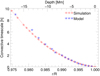 |
Fig. 2. Convective timescale tconv in the upper part of the convection zone from the MHD simulation (red crosses) and a standard solar model (blue stars) (values are taken from Stix 2002). |
2.2. Determination of the boundary of the sunspot flux tube
The sunspot region needs to be clearly defined when the structure of the magnetic flux tube of the sunspot is to be analysed. To do this, we used the magnetic field strength,  . At each of the 25 depth positions from z = 0 Mm to z = −15 Mm, an individual value of the magnetic field strength was determined as a contour value to define the boundary of the magnetic flux tube.
We applied two different methods to determine the contour values. The first method is an estimate of the boundary by eye. The values Beye(z) were chosen to obtain the best match between the contours and the magnetic flux tube at the individual depths. To this end, contours for different B values were visualised on horizontal B maps, clipped to B ≤ 6 kG, for arbitrary time steps. We then chose the contour that best represented the visual contrast between the magnetic flux tube and the non-magnetic surroundings. The obtained values, determined in steps of Δz = 1.25 Mm, are shown in Fig. 3 as blue stars and are listed in Table A.1. This manual method is neither consistent nor applicable to the large number of contours.
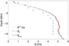 |
Fig. 3. Contour values of the magnetic field strength (Beye(z) and Bc(z)) used to determine the sunspot boundary by eye (blue) and from the maximum magnetic field strength (red). |
As second method we applied an automatic procedure to determine the threshold Bc(z). The maximum magnetic field strength Bmax(z, t) was determined for each grid layer and each time step. Bmax(z, t) was boxcar-smoothed with a width of 240 km in vertical direction and a width of 75 min in time around a defined depth position in steps of Δz = 0.625 Mm. From the smoothed values, averages,  , over all times and ten adjacent depth layers were calculated. These values were divided by 2e to yield the threshold Bc(z),
 (3)
(3)
We made tests for multiples of e in visualising the different contours on horizontal B maps for three different times of 0 h, 15 h, and 27.75 h and for depths in steps of Δz = 1.25 Mm. The best representation of the boundary of the magnetic flux tube throughout the different depth positions was found for a fraction of 2e of  . With this choice, the contours from Bc and Beye match fairly well, although they are determined independent of each other, but differences exist in a few cases.
The obtained Bc(z)-values are shown as red crosses in Fig. 3 overlaid on the temporal averaged values of the maximum magnetic field strength for each vertical grid layer, Bm, t(z)/2e (black dots). The calculated contour values Bc(z) are given in Table A.1 as well.
We computed the area, A, and perimeter, that is, the length of the contour, C, of the sunspot contours at each depth and time step as follows: We smoothed each map of the magnetic field strength with a width of 5 in x- and y-direction. We applied the values Beye(z) and Bc(z) to determine the contours.
3. Compactness of the sunspot
Because of the filamentary structure of the penumbra, the sunspot is not perfectly circular, as shown in the intensity map in Fig. 4, which corresponds to t = 0 h. A contour, outlining the boundary of the sunspot, is drawn at an intensity level Ic = 0.9In, with the normalised intensity,  , where
  denotes the mean intensity of the quiet Sun. A similar structure can be found in maps of the magnetic field strength at 1.25 Mm below the surface. This is shown for the same time step in Fig. 5a. The outer boundary of the flux tube, shown in red, is determined with the automated procedure as described in Sect. 2.2. At this depth, the flux tube is embedded in a mesh-like structure that covers the moat. This structure terminates at the network boundary. This network boundary is seen throughout all depth layers, as displayed in Figs. 5b–f, meaning that the sunspot is embedded in the centre of a moat cell (see also Rempel 2015). We note that in Fig. 5 the field of view is reduced to focus on the sunspot and the moat.
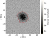 |
Fig. 4. Intensity map at τ = 1 with a contour line at Ic = 0.9In indicating the boundary of the sunspot. |
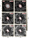 |
Fig. 5. Maps of the magnetic field strength at t = 0 h, shown at different depths (indicated in red in each panel). The boundary of the sunspot (red line) is defined by depth-dependent values of the magnetic field strength. |
Field-free regions penetrate the flux tube. In deeper regions, the average diameter of the flux tube decreases and the field strength increases. In addition, the boundary of the tube becomes more ragged, and the indentations at the boundary penetrate deeper into the inner part of the flux tube. This is most prominent at depths of z = −3.75 Mm and z = −6.25 Mm, as shown in Figs. 5b and c, respectively. The flux tube is more compact in deeper regions, that is, the outer boundary becomes smoother (see Figs. 5d–f).
In time, the ragged structure of the flux tube becomes more pronounced. This is shown in Fig. 6 for a depth of z = −7.5 Mm with a cadence of 6 hours between the snapshots, covering the 30 hours of the analysed data. An animation with a cadence of 15 min for selected depths is provided online.
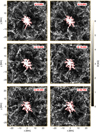 |
Fig. 6. Maps of the magnetic field strength at z = −7.5 Mm at different times (indicated in red in each panel). The boundary of the sunspot (red line) is defined by the contour value Bc = 4781 G. |
At the beginning of the analysis, at t = 0 h (see Fig. 6a) the inner part of the flux tube is mainly undisturbed. Within 6 hours, regions of weaker field appear in the innermost part of the flux tube while the outer structure becomes more ragged, as is shown in Fig. 6b. The increasing raggedness causes a degradation of the flux tube. This degradation process continues in time, as Figs. 6c–e show. At 29.75 h, the roundish structure of the flux tube has completely vanished. The degradation process takes place in all regions deeper than 1 Mm below the surface (see the animation online).
3.1. Method
For a quantitative description of the degradation process, we define the compactness, K, as the ratio of the circumference,  , that corresponds to a circle with the area A, and the actual perimeter, C, around the magnetised area A, that is, the length of the contour with area A,
 (4)
(4)
This enables a comparison of different depths as the average diameter of the flux tube decreases with depth. Thus, a circular flux tube has K = 1. The compactness K(z, t) was calculated for all time steps and all selected depths.
For an increasing raggedness, as discussed in context of Fig. 6, the length of the contour increases. This causes a decrease in the compactness K in time, as described by Eq. (4).
3.2. Results
The compactness in time for eight selected depths is shown in Fig. 7. The compactness evolution for all other analysed depths is shown in Figs. B.1 and B.2. The determination of the sunspot boundary might affect the results. Therefore we analysed a sunspot boundary with both contour values, Bc and Beye (see Sect. 2.2 and Fig. 3, red crosses and blue stars, respectively). However, the analysis with Beye was only performed for depths in steps of Δz = 1.25 Mm. Therefore no values are available at a depth of z = −1.875 Mm, for instance. If not explicitly noted otherwise, the following analysis describes the results obtained with Bc(z).
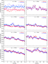 |
Fig. 7. Compactness of the sunspot (normalised area-perimeter ratio) in time, shown at different depths. The boundary of the sunspot is determined with depth-dependent contour values Bc(z) (red crosses) and Beye(z) (blue stars). Degradation times are calculated from linear fits (magenta and cyan lines). |
At the surface, the compactness of the flux tube is almost constant (see Fig. 7a). The scattering of the values is caused by the arbitrary change in filamentary structure of the penumbra. At z = −0.625 Mm the compactness is much smaller than at other depths (see Fig. B.1a). Here, the area of the sunspot is overestimated. The contour value Bc(−0.625 Mm) is not able to reproduce the sunspot boundary. It includes small magnetic structures of the surrounding region. Thus, a higher value for the area leads to a smaller compactness (see Eq. (4)). In conclusion, these results and the visual impression of the sunspot in maps of the magnetic field strength lead to the picture of an overall stable sunspot above z = −1 Mm. This agrees with the evolution of the sunspots magnetic flux at the surface, which is almost stationary, according to Rempel (2015). Below z = −1 Mm, the compactness decreases, as we show in Figs. 7b–h and Figs. B.1b–h and B.2.
The initial compactness differs for different depths. A minimum compactness is found 3.75 Mm below the surface (see Fig. 7c). Towards higher and deeper regions the compactness is larger. The maximum compactness is found at the lowest analysed depth, that is, 15 Mm below the surface. This means that at the beginning of the analysis, the sunspot structure is ragged most strongly at 3.75 Mm below the surface. This agrees with the first visual impression obtained from maps of the magnetic field strengths as described above and shown in Fig. 5.
A similar compactness is found for an analysis with different contour values, that is, Bc(z) and Beye(z). The compactness evolutions for the individual depths resemble each other. We can therefore assume that the exact determination of the sunspot boundary does not substantially affect the analysis of the sunspot compactness. The decrease in compactness in time for all depths reproduces the increase in raggedness, as described above. The evolution of the compactness can be approximated by a linear fit (magenta and cyan lines in Fig. 7), despite the non-continuous decrease. The gradients of the fits show that the compactness does not decrease at the same rate at different depths.
Degradation time of the sunspot. A decrease in compactness describes an increase in raggedness of the flux tube. A higher raggedness causes an increase in the outer surface of the flux tube. Thus, the contact area of the magnetic flux tube with the non-magnetic surrounding plasma increases. This enables a stronger effect of the surroundings, that is, plasma motions. We approximated the evolution of the compactness by a linear fit (see Fig. 7) to calculate a degradation time of the sunspot by the time at which the initial value of the fit has dropped by a factor of 1/e.
Above z = −1 Mm the compactness is stable, as described and concluded above. Therefore the following analysis focuses on layers deeper than 1 Mm below the surface. The degradation time is calculated for the same depths as the compactness. We also used the compactness obtained for both methods, that is, a determination of the flux tube with Bc and Beye, to calculate the degradation times. A similar distribution of the degradation times with depth can be found for Bc and Beye as shown in Fig. 8 (red crosses and blue stars, respectively). Error bars show the standard deviation obtained from the linear fits. Discrepancies between the degradation times when applying different contour values for individual depths can be ascribed to the evolution of the field strength within the flux tube. For times t ≥ 20 h at depths between 3 Mm and 5 Mm below the surface, the contours of the flux tube obtained with the different methods are significantly different. Figure 9 shows a map of the magnetic field strength at a depth of 3.75 Mm below the surface at t = 20 h where the contour lines obtained with the two methods differ significantly. This is one of the few cases where the automatic and manual contours do not match: The higher value of Bc (red) excludes two regions that are included when Beye (blue) is applied. This affects the determined compactness and leads to the deviation of the degradation times for Bc and Beye.
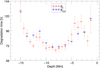 |
Fig. 8. Degradation time of the sunspot at different depths from the compactness of the flux tube. The analysis was made with different depth-dependent contour values Bc(z) and Beye(z) to determine the sunspot boundary (see Sect. 2.2). |
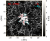 |
Fig. 9. Map of the magnetic field strength at z = −3.75 Mm, at t = 20 h. The outlined contour of the sunspot is determined with Bc = 3500 G (red) and Beye = 2500 G (cyan). |
The structure of the flux tube evolves fastest in regions between 6.25 Mm and 10 Mm below the surface. There, we measure the fastest degradation times of less than three days, as Fig. 8 shows. The slowest decrease in compactness of the flux tube is found at a depth of 15 Mm with a maximum degradation time of 5.4 days.
4. Stability of the sunspot
To understand the decay process of a sunspot, we took stabilising as well as destabilising effects into account. To do this, we studied the stability of the simulated sunspot in the convection zone.
4.1. Methods
The stability of a magnetic flux tube in the upper convection zone is affected by two main effects: The stratification of the thermodynamic properties such as density within the flux tube and in the direct surroundings, and the curvature of the outer surface of the flux tube defining the sunspot. Meyer et al. (1977) described the stability of a flux tube in the upper convection zone and took both effects into account (see Sect. 1). We used Eq. (1) to study the stability of the flux tube of the simulated sunspot in the convection zone. To do this, we determined the following parameters: (1) The density difference in the flux tube, ρs, and the surroundings, ρqs, as a function of depth. (2) The inclination angle, χ, of the outer surface of the flux tube towards the vertical and its radius of curvature, Rc. Both parameters are obtained from a surface function that describes the radial extension of the sunspot with depth.
4.1.1. Density stratification in the upper convection zone
From observations we know that temperature, pressure, and density within a sunspot are lower than in the surrounding quiet Sun. However, this only holds for regions close to the surface. In deeper regions, these differences are expected to decrease (e.g., Jahn & Schmidt 1994; Schlichenmaier 1997). We determined spatial averages of the density for all defined depths z and all time steps for the areas covered by the flux tube of the sunspot and the quiet Sun. The relative density difference between the two regions, (ρqs − ρs)/ρqs, decreases with increasing depth, as Fig. 10 shows for time-averaged values. Because we averaged the spot density over umbra and penumbra, the resulting density contrast just beneath the surface is affected by the Wilson depression, which leads to very low densities in the umbra. Together with a misinterpretation of the flux tube contour, this leads to the discontinuities at z ≥ −0.625 Mm.
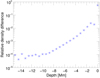 |
Fig. 10. Relative density difference between the quiet Sun and the magnetic flux tube, time-averaged, at different depths. |
4.1.2. Surface function of the flux tube
We define an equivalent radius of the flux tube as the radius,  , of a circle with the same area (see Sect. 3.1). The equivalent radius, re(z, t), is calculated for all defined depths z and all 120 time steps. These individual values are shown in Fig. 11 as rainbow-coloured dots. To approximate the depth dependence, we constructed an asymptotic function,
 (5)
(5)
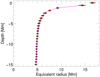 |
Fig. 11. Radial extension of a circular flux tube at different depths obtained from the area A of the simulated sunspot. The time-averaged values (black stars) of all 120 time steps (rainbow-coloured dots, red to blue in time) are fitted by an asymptotic function (magenta line). |
with fitting parameters, ai. The calculation was made for all 120 time steps with re(z, t) over a depth range from z = −0.625 Mm to z = −15 Mm. Figure 11 shows the best-fit function (magenta line), obtained from time-averaged equivalent radii (black stars). The obtained parameters for this fit function are a0 = −10.38 Mm−1, a1 = −2.74 Mm, a2 = −0.22 Mm, a3 = 1.85 Mm−2, and a4 = 4.34 Mm with  as the goodness of the fit (gof).
Inclination angle χ: The inclination angle χ is calculated from the derivative of the surface function with
 (6)
(6)
At each depth position z≤ −0.625 Mm and for each time step the spatial derivative  is calculated. A minimum angle of less than 1.7° is found at the lower-most depth, that is, 15 Mm below the surface. The inclination angle slowly increases towards the surface and reaches 13° at z = −5 Mm. Then, in the upper 5 Mm of the convection zone the increase steepens and almost reaches 85° at z = −0.625 Mm.
Radius of curvature Rc: To calculate the radius of curvature, the first and second derivatives,  and
and  , respectively, of the surface function have to be calculated. It is then determined for each depth position z≤ −0.625 Mm and time step individually with
 (7)
(7)
The radius of curvature is largest at the lowest measurement point, that is, 15 Mm below the surface (see Fig. 12). The flux tube is almost vertical there, thus, the curvature of the flux tube is smallest. The radius of curvature decreases with decreasing depth and has a minimum at z = −2.5 Mm. Upward of the minimum, the radius of curvature increases again. Because of the misinterpretation of the sunspot boundary at z = −0.625 Mm (see Sect. 3.2), the corresponding Rc values show a large scatter, but the trend of an upward-increasing curvature radius is obvious.
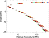 |
Fig. 12. Radius of curvature at different depths, time-averaged (black stars) over all 120 time steps (rainbow-coloured dots, blue to red in time). |
Another parameter necessary to apply the stability criterion, that is, Eq. (1), to the simulated sunspot is the magnetic field strength B(z, t). It is obtained as spatial average over the area of our flux tube contours for each time step t and each selected depth z.
4.2. Results
The stability of the sunspot at the different depth positions and for all time steps was studied by evaluating Eq. (1) with g = 274 m s−1. When the difference on the left side of Eq. (1) is positive, then the flux tube is stable. The difference obtained for the different depths and time steps is visualised in Fig. 13 as dots.
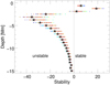 |
Fig. 13. Stability criterion of the sunspot flux tube at different depths time-averaged (black stars) over all 120 time steps (rainbow-coloured dots, blue to red in time). Positive values refer to a stable magnetic flux tube, and negative values represent an unstable configuration. |
Down to z = −1.25 Mm the difference is positive (see Fig. 13), and this means that the flux tube is stable. At z = −1.875 Mm the time-averaged value is still positive, although individual time steps are negative, indicating an instability of the flux tube at these time steps. At greater depth, for z < − 2.5 Mm, the flux tube is found to be unstable for all time steps. The change from stable to unstable is almost always located at the same depth as the smallest radius of curvature, Rc, of the sunspot flux tube. At this depth the surface function has an inclination angle, χ, between 42° and 62° with a temporal average of 46°. The difference reaches a minimum at z = −3.125 Mm. There, the flux tube is most unstable. With increasing depth, the negative difference approaches zero. However, the flux tube does not reach a stable configuration down to the lowest measurement point.
Figure 13 shows that the coloured dots for each depth do not follow the rainbow pattern. This means that no time-dependent relation of the flux-tube stability can be found.
5. Discussion
We applied the stability criterion that was derived with a simple magneto-static model by Meyer et al. (1977) in a current numerical simulation. We find that our simulated sunspot is stable in the upper 2 Mm below the photosphere. Our analysis of the compactness of the flux tube shows that the compactness of the sunspot is constant at the surface. For layers deeper than z = −1.25 Mm, the compactness decreases in time. Meyer et al. (1977) have suspected that a sunspot flux tube could be stable up to a depth of 2 Mm, although their magneto-static model only extended down to 0.650 Mm below the photosphere. In these layers, the inclined magnetic field is predominately kept together by buoyancy forces. The density difference between the magnetic flux tube and the surroundings stabilises the sunspot.
In deeper layers, the stability criterion yields an unstable configuration, as shown in Fig. 13. This represents the increasing effect of fluting. The flux tube is least stable at around z = −3 Mm, whereas the fastest decrease in compactness is found in deeper layers (see Fig. 8). We conjecture that the interchange process is damped within this region. Above z = −1.5 Mm, the field lines are held together by buoyancy to a stable configuration. Magnetic tension affects the behaviour of the field lines in deeper layers. These non-local effects are not taken into account in the linear stability analysis. The field lines can move more freely at larger depths. Therefore the decrease in compactness is faster in layers below z = −3 Mm. It proceeds most rapidly between z = −5 Mm and z = −10 Mm (see Fig. 8).
In even deeper layers, the decrease in compactness is found to proceed more slowly, and the instability of the flux tube approaches a marginally stable state (see Fig. 13). This behaviour is caused by a combination of two effects: (1) The convective timescale increases with depth, as described in Sect. 2.1 and shown in Fig. 2. This leads to the slower action of destabilising forces. (2) The flux tube is more vertical and less strongly curved, which makes it less susceptible to fluting, an effect that has been predicted by Meyer et al. (1977).
The existence of the fluting stability alone is not sufficient for sunspot decay. In addition, turbulent flows are required that remove flux from the spot. Rempel (2015) found a stabilising effect of the moat cell that developed around the simulated sunspot. Below the penumbra, the spot is surrounded by an annulus of upflowing plasma that has a strongly reduced convective rms velocity and is almost devoid of downflows. This strongly inhibits turbulent transport and in particular prevents the submergence of field lines below the penumbra, which would be required for a decay of the penumbra.
A non-monolithic sunspot flux tube was proposed by Parker (1979). He described the individual field lines of a sunspot that are to be kept together in the photosphere. The observable monolithic structure would be divided into several smaller flux bundles approximately 1 Mm below the visible photosphere.
The formation of intrusions at the sunspot boundary, which penetrate the flux tube below the visible surface, was also found by Panja et al. (2021). They calculated MHD simulations with different initial values for the vertical magnetic field at the bottom boundary of their simulation domain. After about 10 hours, the sunspots simulated by Panja et al. (2021) showed a fragmentation of the subsurface field that was substantially stronger than what we found here. This might be due to their more shallow domain (about 5.5 Mm), which cuts out the deeper part of the spot that is less susceptible to fluting. Despite this difference, they also find that the intrusions evolve fastest in depths below z = −5 Mm. Another critical difference is that their setup did not impose a strongly inclined magnetic field at the top boundary. They found that the fluting instability promotes penumbra formation, which is not the case in our simulation. Switching to a potential field boundary condition leads to a naked spot without penumbra in about half an hour, as shown in Rempel (2015). The fluting instability does lead to a growth of the penumbra over time at the expense of the umbra. This evolution was found in Rempel (2015) and can be seen in intensity maps in the top panels of Fig. 14. This points in the same direction as the findings of Panja et al. (2021): The intrusions cause a conversion of magnetic flux from the umbra to the penumbra.
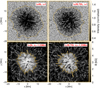 |
Fig. 14. Comparison of the sunspot at the first (t = 0 h, left) and last (t = 29.75 h, right) time step in intensity maps at τ = 1 (top row) and the magnetic field strength at a depth of 1.25 Mm (bottom row). The outlined contours are determined with Ic = 0.9In and Bc = 1669 G. |
The observational study of the decay of a sunspot by Benko et al. (2018) showed that the decrease in magnetic field strength within the umbra is one of the first observable effects of sunspot decay. In time, regions of weaker field are occupied by the penumbra or granulation. Benko et al. (2018) concluded that the umbral area decreases during the decay phase of the sunspot. In our simulation the intrusions of field free plasma that are most prominent at a depth of a few Mm do lead to a visible imprint at the surface (see Fig. 14). While we do not see fully developed light bridges, we find penumbral intrusions and clusters of higher umbral dot density associated with the subsurface fluting. This suggests that subsurface decay does not remain hidden from the surface.
We conjecture that the degradation of the sunspot at its outer surface will in time lead to the separation of the large magnetic flux tube into smaller ones. Light bridges that are observed as the onset of the decay could be caused by such intrusions. The weak magnetic field found within the sunspot in regions above z = −5 Mm, at t ≥ 20 h is the first indication of such a scenario. This agrees with the observations reported by McIntosh (1981) that the process that leads to sunspot decay should already act before the sunspot has fully developed. An interesting property of the simulated sunspot is that the total flux remains constant in spite of the subsurface decay, which can be attributed to the stabilising buoyancy of the penumbra and the stabilising effect of the moat cell. We conjecture that this confinement will eventually fail and at that time lead to a rapid disappearance of the already heavily corrugated spot.
6. Conclusion
We report the following main results from our study: (1) The convective timescale (see Fig. 2), increases with depth and reaches a value of 8 hours at z = −15 Mm, (2) the compactness of the sunspot decreases fastest at a depth around z = −8 Mm (see Fig. 8), and (3) our stability analysis reveals that the sunspot is stable down to approximately −2 Mm and most unstable around z = −3 Mm (see Fig. 13). This leads to a consistent picture of sunspot stability and decay.
Our analysis shows that sunspot (in)stability and decay is an interplay between stabilising and destabilising forces as well as timescales. Buoyant inclined field lines just beneath the photosphere stabilise the sunspot and keep the field lines together. Non-local magnetic tension effects damp the fluting instability in the adjacent layers. In even deeper layers, the fluting instability steadily decreases the compactness of the flux tube. Thus, the spot eventually loses its coherency in layers between z = −5 Mm and z = −10 Mm. Deeper layers are less strongly affected because the destabilising force is weaker, convective timescales (time of change) increase substantially with depth, and the moat cell is stabilising.
We recall that this scenario of sunspot decay is based on simulated data. The described process occurs within the upper convection zone, a region hidden from real observations. For a more detailed clarification of the decay process, we might therefore have to compare characteristics of observations with those seen in the photospheric region of the simulated sunspot. Tracers of the degradation process that are visible in the photosphere could then be studied in greater detail in real observations. We propose to take light bridges as tracers for the indentations at the boundary of the flux tube below the solar surface into account. Panja et al. (2021) reported that upflows within the intrusions become visible as light bridges at the surface. The role of MMFs in the sunspot decay process has been discussed in many studies (see Sect. 1). Their connection to the sunspot should be studied in simulations. In simulations we can take advantage of tracing the connection of their field lines below the surface. This might give insight into a possible role of these features in the interchange and degradation process of a sunspot.
Movie
Movie 1 associated with Fig. 6 (BMaps) Access Supplementary Material
Acknowledgments
We gratefully acknowledge fruitful discussions with Nazaret Bello González and Markus Schmassmann, and we thank Rebecca Centeno Elliott for carefully reading and commenting on the manuscript. We appreciate the useful comments and suggestions of the anonymous referee. H. S. has been funded by the Deutsche Forschungsgemeinschaft, under grant No. RE 3282 and acknowledges financial support from the HAO visitor program. This material is based upon work supported by the National Center for Atmospheric Research, which is a major facility sponsored by the National Science Foundation under Cooperative Agreement No. 1852977.
References
- Benko, M., González Manrique, S. J., Balthasar, H., et al. 2018, A&A, 620, A191 [NASA ADS] [CrossRef] [EDP Sciences] [Google Scholar]
- Bumba, V. 1963, Bull. astr. Inst. Czechosl., 14, 91 [Google Scholar]
- Harvey, K., & Harvey, J. 1973, Sol. Phys., 28, 61 [NASA ADS] [CrossRef] [Google Scholar]
- Jahn, K. 1992, in Sunspots: Theory and Observations, eds. J. H. Thomas, & N. O. Weiss (Dordrecht: Springer Netherlands), 139 [Google Scholar]
- Jahn, K. 1997, in 1st Advances in Solar Physics Euroconference. Advances in Physics of Sunspots, eds. B. Schmieder, J. C. del Toro Iniesta, & M. Vazquez, PASPC, 118, 122 [Google Scholar]
- Jahn, K., & Schmidt, H. U. 1994, A&A, 290, 295 [NASA ADS] [Google Scholar]
- Kubo, M. 2012, in 4th Hinode Science Meeting: Unsolved Problems and Recent Insights, eds. L. Bellot Rubio, F. Reale, & M. Carlsson, PASPC, 455, 49 [Google Scholar]
- Kubo, M., Shimizu, T., & Tsuneta, S. 2007, ApJ, 659, 812 [Google Scholar]
- Kurucz, R. 1993, ATLAS9 Stellar Atmosphere Programs and 2 km/s grid. Kurucz CD-ROM No. 13. Cambridge, 13 [Google Scholar]
- Martínez Pillet, V. 2002, Astron. Nachr., 323, 342 [NASA ADS] [CrossRef] [Google Scholar]
- Martínez Pillet, V., Moreno-Insertis, F., & Vazquez, M. 1993, A&A, 274, 521 [NASA ADS] [Google Scholar]
- McIntosh, P. S. 1981, in The Physics of Sunspots, eds. L. E. Cram, & J. H. Thomas, 7 [Google Scholar]
- Meyer, F., Schmidt, H. U., Weiss, N. O., & Wilson, P. R. 1974, MNRAS, 169, 35 [NASA ADS] [CrossRef] [Google Scholar]
- Meyer, F., Schmidt, H. U., & Weiss, N. O. 1977, MNRAS, 179, 741 [NASA ADS] [Google Scholar]
- Panja, M., Cameron, R. H., & Solanki, S. K. 2021, ApJ, 907, 102 [Google Scholar]
- Parker, E. N. 1979, ApJ, 230, 905 [NASA ADS] [CrossRef] [Google Scholar]
- Petrovay, K., & Moreno-Insertis, F. 1997, ApJ, 485, 398 [NASA ADS] [CrossRef] [Google Scholar]
- Petrovay, K., & van Driel-Gesztelyi, L. 1997, Sol. Phys., 176, 249 [NASA ADS] [CrossRef] [Google Scholar]
- Priest, E. 2014, Magnetohydrodynamics of the Sun (Cambridge University Press) [Google Scholar]
- Rempel, M. 2012, ApJ, 750, 62 [NASA ADS] [CrossRef] [Google Scholar]
- Rempel, M. 2015, ApJ, 814, 125 [NASA ADS] [CrossRef] [Google Scholar]
- Schlichenmaier, R. 1997, PhD Thesis, Ludwig-Maximilians-Universität München, Germany [Google Scholar]
- Schlüter, A., & Temesváry, S. 1958, Symp. - IAU, 6, 263 [Google Scholar]
- Schüssler, M. 1984, A&A, 140, 453 [NASA ADS] [Google Scholar]
- Sheeley, N. R. 1969, Sol. Phys., 9, 347 [NASA ADS] [CrossRef] [Google Scholar]
- Shine, R., & Title, A. 2000, in Encyclopedia of Astronomy and Astrophysics, ed. P. Murdin (Bristol: Institute of Physics Publishing), 2038 [Google Scholar]
- Simon, G. W., & Leighton, R. B. 1964, ApJ, 140, 1120 [NASA ADS] [CrossRef] [Google Scholar]
- Simon, G. W., & Weiss, N. O. 1970, Sol. Phys., 13, 85 [NASA ADS] [CrossRef] [Google Scholar]
- Solanki, S. K. 2003, A&ARv, 11, 153 [Google Scholar]
- Stix, M. 2002, The Sun, A&A Library (Berlin Heidelberg: Springer) [Google Scholar]
- Strecker, H. 2020, PhD Thesis, Albert-Ludwigs-Universität Freiburg, Germany [Google Scholar]
- Thomas, J. H., Weiss, N. O., Tobias, S. M., & Brummell, N. H. 2002, Nature, 420, 390 [NASA ADS] [CrossRef] [PubMed] [Google Scholar]
- van Driel-Gesztelyi, L., & Green, L. M. 2015, Liv. Rev. Sol. Phys., 12, 1 [NASA ADS] [CrossRef] [Google Scholar]
- Verma, M., Balthasar, H., Deng, N., et al. 2012, A&A, 538, A109 [NASA ADS] [CrossRef] [EDP Sciences] [Google Scholar]
- Zhang, H., & AI, G., Wang, H., Zirin, H., & Patterson, A., 1992, Sol. Phys., 140, 307 [Google Scholar]
Appendix A: Determination of the flux tube boundary
Threshold levels Bc and Beye for determining the boundary of the sunspot in maps of the magnetic field strength for defined depths z.
Appendix B: Compactness of the flux tube
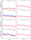 |
Fig. B.1. Compactness of the sunspot (normalised area-perimeter ratio) in time, shown at different depths. The boundary of the sunspot is determined with depth-dependent contour values Bc(z) (red crosses) and Beye(z) (blue stars). Same as Fig. 7. |
All Tables
Threshold levels Bc and Beye for determining the boundary of the sunspot in maps of the magnetic field strength for defined depths z.
All Figures
|
Fig. 1. Geometry of a magnetic flux tube (Vf) embedded in field-free plasma (Vp) (image adapted from Meyer et al. 1977). |
| In the text | |
|
Fig. 2. Convective timescale tconv in the upper part of the convection zone from the MHD simulation (red crosses) and a standard solar model (blue stars) (values are taken from Stix 2002). |
| In the text | |
|
Fig. 3. Contour values of the magnetic field strength (Beye(z) and Bc(z)) used to determine the sunspot boundary by eye (blue) and from the maximum magnetic field strength (red). |
| In the text | |
|
Fig. 4. Intensity map at τ = 1 with a contour line at Ic = 0.9In indicating the boundary of the sunspot. |
| In the text | |
|
Fig. 5. Maps of the magnetic field strength at t = 0 h, shown at different depths (indicated in red in each panel). The boundary of the sunspot (red line) is defined by depth-dependent values of the magnetic field strength. |
| In the text | |
|
Fig. 6. Maps of the magnetic field strength at z = −7.5 Mm at different times (indicated in red in each panel). The boundary of the sunspot (red line) is defined by the contour value Bc = 4781 G. |
| In the text | |
|
Fig. 7. Compactness of the sunspot (normalised area-perimeter ratio) in time, shown at different depths. The boundary of the sunspot is determined with depth-dependent contour values Bc(z) (red crosses) and Beye(z) (blue stars). Degradation times are calculated from linear fits (magenta and cyan lines). |
| In the text | |
|
Fig. 8. Degradation time of the sunspot at different depths from the compactness of the flux tube. The analysis was made with different depth-dependent contour values Bc(z) and Beye(z) to determine the sunspot boundary (see Sect. 2.2). |
| In the text | |
|
Fig. 9. Map of the magnetic field strength at z = −3.75 Mm, at t = 20 h. The outlined contour of the sunspot is determined with Bc = 3500 G (red) and Beye = 2500 G (cyan). |
| In the text | |
|
Fig. 10. Relative density difference between the quiet Sun and the magnetic flux tube, time-averaged, at different depths. |
| In the text | |
|
Fig. 11. Radial extension of a circular flux tube at different depths obtained from the area A of the simulated sunspot. The time-averaged values (black stars) of all 120 time steps (rainbow-coloured dots, red to blue in time) are fitted by an asymptotic function (magenta line). |
| In the text | |
|
Fig. 12. Radius of curvature at different depths, time-averaged (black stars) over all 120 time steps (rainbow-coloured dots, blue to red in time). |
| In the text | |
|
Fig. 13. Stability criterion of the sunspot flux tube at different depths time-averaged (black stars) over all 120 time steps (rainbow-coloured dots, blue to red in time). Positive values refer to a stable magnetic flux tube, and negative values represent an unstable configuration. |
| In the text | |
|
Fig. 14. Comparison of the sunspot at the first (t = 0 h, left) and last (t = 29.75 h, right) time step in intensity maps at τ = 1 (top row) and the magnetic field strength at a depth of 1.25 Mm (bottom row). The outlined contours are determined with Ic = 0.9In and Bc = 1669 G. |
| In the text | |
|
Fig. B.1. Compactness of the sunspot (normalised area-perimeter ratio) in time, shown at different depths. The boundary of the sunspot is determined with depth-dependent contour values Bc(z) (red crosses) and Beye(z) (blue stars). Same as Fig. 7. |
| In the text | |
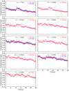 |
Fig. B.2. Same as Fig. B.1, but for different depths. |
| In the text | |
Current usage metrics show cumulative count of Article Views (full-text article views including HTML views, PDF and ePub downloads, according to the available data) and Abstracts Views on Vision4Press platform.
Data correspond to usage on the plateform after 2015. The current usage metrics is available 48-96 hours after online publication and is updated daily on week days.
Initial download of the metrics may take a while.