| Issue |
A&A
Volume 649, May 2021
|
|
|---|---|---|
| Article Number | A117 | |
| Number of page(s) | 15 | |
| Section | Cosmology (including clusters of galaxies) | |
| DOI | https://doi.org/10.1051/0004-6361/202039781 | |
| Published online | 26 May 2021 | |
Properties of gas phases around cosmic filaments at z = 0 in the IllustrisTNG simulation
Université Paris-Saclay, CNRS, Institut d’astrophysique spatiale, 91405 Orsay, France
e-mail: This email address is being protected from spambots. You need JavaScript enabled to view it.
Received:
28
October
2020
Accepted:
4
March
2021
Abstract
We present the study of gas phases around cosmic-web filaments detected in the TNG300-1 hydro-dynamical simulation at redshift z = 0. We separate the gas into five different phases according to temperature and density. We show that filaments are essentially dominated by gas in the warm-hot intergalactic medium (WHIM), which accounts for more than 80% of the baryon budget at r ∼ 1 Mpc. Apart from WHIM gas, cores of filaments (r ≤ 1 Mpc) also host large contributions from other hotter and denser gas phases, whose fractions depend on the filament population. By building temperature and pressure profiles, we find that gas in filaments is isothermal up to r ∼ 1.5 Mpc, with average temperatures of Tcore = 4−13 × 105 K, depending on the large-scale environment. Pressure at cores of filaments is on average Pcore = 4−12 × 10−7 keV.cm−3, which is ∼1000 times lower than pressure measured in observed clusters. We also estimate that the observed Sunyaev-Zel’dovich signal from cores of filaments should range between 0.5 < y < 4.1 × 10⁻⁸, and these results are compared with recent observations. Our findings show that the state of the gas in filaments depends on the presence of haloes and on the large-scale environment.
Key words: large-scale structure of Universe / methods: statistical / methods: numerical
© D. Galárraga-Espinosa et al. 2021
 Open Access article, published by EDP Sciences, under the terms of the Creative Commons Attribution License (https://creativecommons.org/licenses/by/4.0), which permits unrestricted use, distribution, and reproduction in any medium, provided the original work is properly cited.
1. Introduction
Under the action of gravity, matter is assembled to form a gigantic network composed of nodes, filaments, walls, and voids called the cosmic web (de Lapparent et al. 1986; Bond et al. 1996). This structure is mainly set by the dynamics of dark matter (DM), which builds the cosmic skeleton, and baryonic matter is accreted onto the DM skeleton driven by gravity. Studies based on simulations have shown that cosmic filaments might contain almost 50% of the mass of the Universe (e.g., Cautun et al. 2014), so our understanding of matter in the Universe is closely tied to that of filaments.
Along with gravity and because of their collisional nature, baryons are also subject to a large variety of physical processes such as heating, cooling, mass ejection, and shocks caused by, for example stellar and AGN feedback, galactic winds, radiation. These processes form a complex cycle in which gas is pushed into different physical states, or phases, which co-exist in the cosmic web and are spatially correlated with the different structures at different cosmic scales (e.g., Ursino et al. 2010; Shull et al. 2012; Cen & Ostriker 2006; Haider et al. 2016; Martizzi et al. 2019; Ramsøy et al. 2021).
Hydro-dynamical numerical simulations are an ideal tool to explore gas in filaments without the difficulties specific to observational data analysis (e.g., foreground contamination, low signal-to-noise ratio, and redshift uncertainties). These have significantly improved understanding of the properties of baryons and the processes to which they are subjected in the cosmic web (e.g., Ursino et al. 2010; Shull et al. 2012; Nevalainen et al. 2015; Gheller et al. 2015, 2016). For example, Gheller & Vazza (2019) investigate the link between the properties of cosmic filaments (e.g., mass, length, and temperature) and the physics deciding the fate of baryons in the cosmic web. Martizzi et al. (2019) analyse the gas content and separated gas into different phases of the various structures of the cosmic web at different redshifts of the IllustrisTNG simulation (Nelson et al. 2019). More recently, Gheller & Vazza (2020) show that one of the most promising tracers of gas in the diffuse warm-hot intergalactic medium (WHIM) around filaments is the Sunyaev-Zel’dovich (SZ) effect, thanks to its linear dependence on gas pressure.
Given that cosmic filaments lack a standard and unique definition and that their mass densities are low in comparison with the nodes of the cosmic web, studies of filaments face all the same limitations in terms of detection and identification. Several algorithms, which detect filaments using various approaches, have been developed to overcome these limitations. For example, filaments can be defined based on the topology of the matter density field, on density thresholds, on the velocity field, or even with a probabilistic approach (see for example Aragón-Calvo et al. 2010; Sousbie 2011; Sousbie et al. 2011; Cautun et al. 2013; Libeskind et al. 2018; Bonnaire et al. 2020; Pereyra et al. 2020).
In the present paper, we study gas around cosmic filaments detected with the DisPerSE algorithm (Sousbie 2011; Sousbie et al. 2011) in the galaxy distribution of the Illustris The Next Generation simulation (IllustrisTNG, Nelson et al. 2019) at redshift zero. We separate the gas into different density and temperature states, called phases, and we study the gas properties around the different populations of filaments identified in Galárraga-Espinosa et al. (2020). We map the distribution of the different baryonic phases around filaments by building phase fraction profiles, and we characterise their thermodynamical properties by means of temperature and pressure profiles. We remove the contamination of gas contained in nodes, and we identify the contribution of massive (Mtot > 1012 M⊙) galactic haloes to explicitly focus on the properties of the gas of filaments that are not associated with smaller-scales collapsed structures.
In Sect. 2, we introduce the IllustrisTNG simulation and we describe the filament catalogue as well as the five different phases studied in this work. We show our results on the distribution of these phases around the different types of filaments in Sect. 3. Section 4 presents a study of the temperature and pressure of the five gas phases around filaments. We analyse, in Sect. 5, the contribution of gas in galactic haloes to the filament temperature and pressure when the haloes are not removed in the analysis. Finally, we estimate the SZ signal from filaments in Sect. 6, and we summarise our conclusions in Sect. 7.
2. Data
2.1. IllustrisTNG simulation
We analyse the gravo-magnetohydrodynamical simulation IllustrisTNG1 (Nelson et al. 2019). This simulation follows the coupled evolution of DM, gas, stars, and black holes from redshift z = 127 to z = 0. IllustrisTNG is run with the moving-mesh code Arepo (Springel 2010) with the cosmological parameters from Planck Collaboration XIII (2016), namely ΩΛ, 0 = 0.6911, Ωm, 0 = 0.3089, Ωb, 0 = 0.0486, σ8 = 0.8159, ns = 0.9667 and h = 0.6774.
In this work, we choose to use the largest simulation volume with the highest mass resolution of the IllustrisTNG suite to accurately describe large cosmic filaments and their gas content down to small scales. We therefore focus on the simulation box TNG300-1 at a redshift z = 0. This box consists in a cube of around 302 Mpc side length with a DM resolution of mDM = 4.0 × 10⁷ M⊙/h and a number of particles of NDM = 25003.
The gaseous component in the IllustrisTNG simulation is implemented by Voronoi cells evolving in time using Godunov’s method (Nelson et al. 2019). Owing to Riemann solvers at the cell interfaces, the Voronoi cells track the conserved quantities of the gas fluid (e.g., mass, momentum, and energy), and they are refined and de-refined according to a mass target of 7.6 × 10⁶ M⊙/h (Springel 2010; Nelson et al. 2019; Weinberger et al. 2020; Pillepich et al. 2018). Finally, the baryonic processes driving gas dynamics (e.g., star formation, stellar evolution, chemical enrichment, gas cooling, black hole formation, growth, and feedback) are implemented in a subgrid manner following the ‘TNG model’ (Pillepich et al. 2018; Nelson et al. 2019). This model was specifically calibrated on observational data to match to the observed galaxy properties and statistics (Nelson et al. 2019). The complete description of this model can be found in Pillepich et al. (2018).
2.2. Filament catalogue
The catalogue of filaments used in this work was constructed in Galárraga-Espinosa et al. (2020), which provides details and technicalities. Here, we simply summarise the main important points.
We detected the filamentary structures in the simulation box by applying DisPerSE (Sousbie 2011; Sousbie et al. 2011) to the galaxy catalogue of the TNG300-1 simulation at z = 0. Galaxies of this catalogue were selected to be in the stellar masses range of 109 ≤ M∗[M⊙] ≤ 1012 in order to correspond to observational limits (Brinchmann et al. 2004; Taylor et al. 2011). From the galaxy distribution, DiPerSE first computes the density field using the Delaunay Tessellation Field Estimator (DTFE, Schaap & van de Weygaert 2000; van de Weygaert & Schaap 2009). To minimise the contamination by shot noise and to prevent the identification of small-scale, possibly spurious, features, following Malavasi et al. (2020), we smoothed the density field by averaging the density value at each vertex of the Delaunay tessellation with the values at the surrounding vertices. The DisPerSE algorithm then identifies the critical points of the density field (points where the gradient of the field is zero) using discrete Morse theory. Filaments are thus defined as sets of segments connecting maximum density critical points to saddles. The user can choose the significance of the detected filaments by fixing the persistence ratio of the corresponding pair of critical points and, following Galárraga-Espinosa et al. (2020), the persistence is fixed to 3σ in this work.
The filaments of the obtained catalogue have a maximum length of Lf = 65.6 Mpc, their minimum is Lf = 0.4 Mpc, and the mean and median lengths are 10.9 and 8.8 Mpc, respectively. As in Galárraga-Espinosa et al. (2020), we separate two statistically distinct populations of filaments, short (Lf < 9 Mpc) and long (Lf ≥ 20 Mpc), depending on the density of their environments in the cosmic web (denser and less dense, respectively). In addition, we consider here medium-length filaments (9 ≤ Lf < 20 Mpc) to study gas around all the filaments of our catalogue. These specific length boundaries are not sharply defined because they weakly depend on the density of the tracers of the matter distribution, which in our case is the number of galaxies in the simulated volume (10−2 gal Mpc−3). However, the results we show here do not depend on the exact values of these length boundaries.
2.3. Gas cell dataset
The TNG300-1 simulation box provides a dataset of 15 625 000 000 gas cells. Because we want to study gas properties that are associated with filaments, we removed from the analysis the cells located within spheres of radius 3 × R200 centred on the position of the maximum density critical points of the Delaunay density field (hereafter CPmax, see Sect. 2.2), which are the topological nodes of the skeleton. This step removes 11% of the initial dataset. For illustration, the gas cells within 1 × R200 of the CPmax are represented by the red points in the xy slice of Fig. 1.
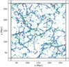 |
Fig. 1. Two-dimensional projection of a slice of thickness 50 Mpc in the xy plane of the TNG300-1 box. The red points correspond to gas cells within the R200 radii of nodes (traced in this work by the DisPerSE maximum density critical points, see Sect. 2.3). The blue points represent gas around filaments, at distances closer than 1 Mpc from the spine of the cosmic web. Finally, the green points show gas in the R200 region of galactic haloes (i.e. within spheres of radius 1 × R200). The galactic haloes residing in filaments are clearly apparent (green over blue regions). The centres of the cells are plotted as points, but the TNG300-1 simulation is described by Voronoi cells having various volumes. |
We also removed the contribution of galactic haloes, which we define as massive (Mtot > 1012 M⊙), collapsed structures hosting at least one galaxy of stellar mass 109 ≤ M∗ ≤ 1012 M⊙ (see green points in Fig. 1). We therefore discarded the gas cells located within spheres of radius 3 × R200 centred on these structures. After these steps, our dataset contains 76% of the initial cells; the other 24% lies within 3 × R200 of nodes (11%) or galactic haloes (13%).
Furthermore, given the excess of critical points near the boundaries of the simulation box, we chose, following Galárraga-Espinosa et al. (2020), to completely disregard the regions of thickness 25 Mpc at the box boundaries (vertical and horizontal lines in Fig. 1), and to replicate the cell distribution at the borders to reduce the effects of a volume-limited simulation in the gas profiles.
By masking the CPmax and the galactic haloes, and by removing the cells at the borders, we obtained a dataset containing ∼6 400 000 000 gas cells (i.e. ∼40% of the initial dataset). This is still an extremely large number, and dealing with such an amount of information is computationally very expensive and time consuming. So, to perform our analysis in reasonable computing time, we sampled the gas dataset by randomly selecting 1 cell out of 500. By doing so, we end up with a final set containing 12 711 272 cells. We checked that this number is representative of the full cell dataset, as different random samples give exactly the same results in terms of gas distributions and statistical properties. Hence, the resulting gas dataset allows us to perform the analysis of properties of gas of the inter-filamentary medium, without contamination of gas in haloes and nodes. This gas dataset is used in the following Sects. 3 and 4, while in Sect. 5, gas in haloes is included to show explicitly how the latter contributes to the baryon content, temperature, and pressure profiles of filaments.
2.4. Cell temperature and pressure
The IllustrisTNG simulation offers information about various properties and characteristics of the gas cells (labelled as PartType0). We derive the temperature and pressure of each cell by employing their corresponding InternalEnergy, ElectronAbundance, and Density fields, hereafter u, xe, and ρcell respectively.
Gas cell temperature is computed under the assumption of perfect monoatomic gas and is written as
 (1)
(1)
In this equation, γ corresponds to the adiabatic index of perfect monoatomic gas (γ = 5/3), kB is the Boltzmann constant, and μ denotes the mean molecular weight. The latter is estimated as follows:
 (2)
(2)
where XH is the hydrogen mass fraction (XH = 0.76) and mp denotes the mass of the proton. In these equations, all the quantities are expressed in the International System of Units.
The thermodynamic pressure is estimated from the temperature and electron density as
 (3)
(3)
The electron density ne, in m−3, is computed as the electron abundance times the hydrogen density, ne = xe × nH, where nH = XH ρcell/mp. We convert the pressure from pascals to the more usual unit in astrophysics of kev.cm−3.
2.5. Definition of gas phases
Gas in the cosmic web is subjected to several complex and interconnected physical processes, which can be essentially summarised by accretion, ejection, heating, and cooling. These processes are not isotropic; they depend on the local environment in the cosmic web and therefore they distribute the gas into different phases. Phases can easily be identified with the help of a phase-space diagram showing the relation between gas temperature and gas density (e.g., Ursino et al. 2010; Shull et al. 2012; Cen & Ostriker 2006; Haider et al. 2016; Martizzi et al. 2019). These phases share neither the same physical properties nor the same spatial distribution as we show below.
In this work, we analyse the baryonic gas not only in terms of the various populations of cosmic filaments we identified, but also in terms of its distribution across five different phases. We consider the five phases of gas presented in Table 1 and in Fig. 2, which show the normalised 2D histogram of the gas cells of the TNG300-1 simulation. The five gas phases are defined according to their hydrogen number density2, nH, and their temperature. These are the diffuse intergalactic medium (diffuse IGM), WHIM, warm circumgalactic medium (WCGM), halo gas, and hot gas. Further details are available in Sect. 2.3 of Martizzi et al. (2019). We note, however, that in our analysis we do not consider star-forming gas, which is defined in Martizzi et al. (2019) as gas with densities higher than nH > 0.13 cm−3, temperatures lower than T < 107 K, and star formation rate SFR > 0. This is motivated by the fact that the ElectronAbundance field (see Sect. 2.4) of star-forming cells is altered by the subgrid model of star formation (Springel & Hernquist 2003) employed in the simulation (see an example in Pakmor et al. 2018). Moreover, it is worth noting that star formation is not a representative property of gas in the IllustrisTNG simulation, as cells with SFR > 0 account for only a tiny fraction of the total gas budget (∼0.1%).
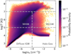 |
Fig. 2. Phase-space of the gas cells in the TNG300-1 simulation, shown by the normalised 2D histogram of the cells. The five different gas phases studied in this work are delimited by the thick dashed lines. They are defined as in Martizzi et al. (2019), and presented in Table 1 and Sect. 2.5. |
Before presenting our results in the next sections, we would like to recall that the boundaries of these phases are somewhat artificial and should not be considered as sharp limits. Gas cells in the neighbourhood of these limits may suddenly move from one phase to another under the influence of even the tiniest perturbation; for example WCGM gas just needs to be heated up to temperatures beyond 107 K to be counted as hot gas. Similarly, gas cells at a given place in the phase diagram may have reached their location through a large variety of processes. For instance, gas within the boundaries of the WCGM phase may correspond to WHIM gas that has been accreted and has become denser, to halo gas that has been heated by feedback effects, or to hot gas that has cooled down. Therefore these density and temperature limits defining the gas phases should simply be considered as guiding references.
3. Distribution of gas phases around filaments
3.1. Gas fraction profiles
In this section, we describe how the various gas phases introduced above are distributed around the filaments of our catalogue (Sect. 2.2). We computed the radial profiles of the mass fraction of each gas phase (hereafter called φi) along the direction perpendicular to the filament spine (hereafter called r). The phase mass fraction is defined as
 (4)
(4)
where ρgas, i(r) corresponds to the mass density of the gas phase i (i= WHIM, WCGM, etc.) at a given location around filaments, and ρgas, tot(r) is the total mass density of gas (all phases included) at this location. These densities are computed as mass averages in volumes of concentric cylindrical shells (denoted by the index k) around the axis of filaments. For all the Nseg filament segments, for a given distance rk from their axes, we summed the masses of the gas cells mcell located inside the cylindrical shells of outer radius rk and of thickness rk − rk − 1 to get the total enclosed gas mass at this location. We then divided this result by the corresponding volume, that is the volume of the hollow cylinder of thickness rk − rk − 1 and of height the total segment length. This is given by
 (5)
(5)
where, N(k) corresponds to the number of cells within the k-th shell around the segment s of length ls. We note that the radial distance r is binned in k = 20 equally spaced logarithmic bins, starting from the filament spine up to 100 Mpc.
The resulting phase fraction profiles φi are presented in Fig. 3 for short, medium-length, and long filaments in the left, middle, and right panels, respectively. The error bars in this figure are obtained by propagating these of the density measurements. The latter are obtained using the bootstrap method, that is we compute the standard deviation of 1000 density profiles, obtained by applying Eq. (5) to a set of Nseg = 1000 randomly extracted (with replacement) filament segments. These errors thus quantify the statistical variance of the density around our limited sample of filaments. In this figure, we distinguish three different regimes for all the filaments:
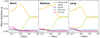 |
Fig. 3. Gas mass fraction profiles φi (see Eq. (4)) of the five different phases (labelled by the index i) around short (left panel), medium-length (centre), and long filaments (right panel). All the gas phases used in this work are presented in Sect. 2.5. |
(i) Far away from the filament spine (at distances r > 10 Mpc), gas is mainly in a diffuse state (more than 95% of the total budget). This is shown by the fractions of diffuse IGM and WHIM gas, which are the highest of all the filaments; as expected, diffuse IGM is the most representative phase (∼50%) at such large distances. In the case of short filaments (left panel of Fig. 3), from outside to inside, we see a decline of the diffuse IGM fraction starting at distances of ∼20 Mpc from the spine, and this goes along with a rise of the fraction of WHIM. This feature can be interpreted as the accretion of diffuse gas to filaments, which starts at these large distances in the short population. Accreted gas is gravitationally heated (as will be shown by the temperature profiles later on), and diffuse IGM gas is thus converted to WHIM, which becomes the dominant phase at r ∼ 20 Mpc from the spine of the filament (see intersection point). However, in long filaments (right panel), this accretion feature happens at distances much closer to the spine because the diffuse IGM and WHIM fractions intersect only at r ∼ 5 Mpc. These differences are likely because short and long filaments reside in different environments of the cosmic web (Galárraga-Espinosa et al. 2020). Short filaments are in denser regions (e.g., in the vicinity of galaxy clusters), where the heating of the gas due to accretion happens at larger radii from the spine than in less dense environments (e.g., in the surroundings of voids), which are traced by long filaments. Finally, the fractions of WCGM, halo, and hot gas are only tiny at these large distances from the spines.
(ii) At intermediate distances (1 < r ≤ 10 Mpc), the accretion of cold and diffuse gas to the core continues. We observe a very significant decrease of the fraction of diffuse IGM, along with an abrupt increase of that of the WHIM phase. The fraction of WHIM reaches its maximum (∼88% of the total baryon budget in short and ∼80% in long filaments) at distances of r ∼ 1 Mpc from the spine. This radial scale of 1 Mpc is independent of the length of the filament and does not depend on the resolution of the simulation either (see Appendix A for details). Thus this points to a more general radial extent of gas in filaments, which might be defined as the radius at which the baryonic processes in filaments (e.g., shocks, feedback effects, and mergers) start counteracting the pure gravitational infall of gas. Moreover, in this radial regime of 1 < r ≤ 10 Mpc, almost all the diffuse IGM gas has been heated and turned into another phase, thereby becoming negligible (less than 5% and decreasing) in the total baryon budget, which is completely dominated by WHIM. There are no significant changes in the denser phases (WCGM, halo and hot gas), whose fractions remain constant and tiny on the outskirts of filaments.
(iii) The cores of filaments (r ≤ 1 Mpc) are characterised by a very sharp decrease of the fraction of WHIM and the increase of the WCGM and hot gas, which remained tiny so far. Precisely, we report in Table 2 the fractions of each gas phase in the first radial bin, that is r = 0.05 Mpc. We notice that, despite the decrease, WHIM remains the dominant phase in all types of filaments (accounting for ∼70% of the baryons), which is in qualitative agreement with previous findings at z = 0, using different simulations and filament finders (e.g., Nevalainen et al. 2015; Cui et al. 2018, 2019; Martizzi et al. 2019; Tuominen et al. 2021). We note that cores of filaments are also composed of hotter and denser gas (WCGM and especially hot gas). As WHIM gas approaches or falls into the filament, it is subjected to a variety of baryonic processes (shocks, feedback effects, and mergers) that are specific to these dense environments, which contain significantly larger numbers of galaxies than the outskirts of filaments (as shown in Galárraga-Espinosa et al. 2020), thus making them susceptible to the effects of galactic physics (see Sect. 5). Moreover, we note that the fractions of the different phases depend on the length of filament, and this is further investigated in the next subsection, where we study, at the cell level, the gas content of cores of the short and long populations.
Mass fractions φi of the different gas phases at the core of short, medium-length, and long filaments.
3.2. Phase diagrams of gas in filaments
We now analyse their gas content by the means of phase diagrams to get a clearer picture of the physical properties of gas in filaments. As we mentioned above, the boundaries between the five phases used in Fig. 3 are somehow arbitrary and must not be considered as sharp limits. This is particularly the case in cores of filaments (and in haloes and nodes) due to the numerous physical processes affecting the gas in these dense regions.
We built the phase diagrams of gas in cylinders of radius 1 Mpc around the spine of filaments. This radius was chosen following the results of Fig. 3 because it corresponds to the distance from which the WHIM fraction starts decreasing, giving room to the other hotter and denser baryonic phases. The phase diagram of cells in filaments is presented in the 2D histogram of Fig. 4 (first panel). For the sake of comparison, we also analysed the phase diagram of gas inside galactic haloes (see definition in Sect. 2.3) and around the DisPerSE CPmax points, which are not counted in the first filament phase diagram. These are presented in the second and third panels of Fig. 4, respectively, where the gas cells within spheres of radius 1 × R200 centred on galactic haloes and on CPmax are displayed.
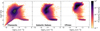 |
Fig. 4. Phase portraits of gas, presenting the normalised 2D histograms of the gas cells in the corresponding structures. First panel: gas in filaments (within 1 Mpc from the core). Second panel: gas within the R200 radius of galactic haloes (defined as haloes of mass Mtot > 1012 M⊙ hosting at least one galaxy of mass 109 ≤ M∗[M⊙] ≤ 1012). Third panel: gas within the R200 radius of the DisPerSE maximum density critical points (CPmax), tracers of nodes. The 68% and 99% contours correspond to results of short (orange) and long filaments (blue), to galactic haloes (dotted green lines), and CPmax (dash-dotted red contours). |
The phase portrait of gas in filaments shows that most of the gas cells in these structures have temperatures and densities corresponding to the WHIM phase, which is in agreement with the previous results of Fig. 3 and Table 2. The contours of short and long filaments (orange and blue lines) are rather circular and share the common region around nH = 10−5.3 cm−3 and T = 106.1 K. However, their overall distribution is significantly different, showing that these two populations of filaments are not made by exactly the same gas. The contours of the long filaments are shifted towards the cooler values with respect to short filaments, and these present a contribution of cold and diffuse IGM gas. The latter corresponds to primordial gas that has never been heated by baryonic processes, and whose temperature is regulated by the competition between radiative heating (by the UV background) and the expansion of the Universe (Valageas et al. 2003). On the other hand, short filaments present larger contributions of hot gas, as expected from these puffy and dense structures. We now comment on the small, but non-negligible, presence of cold and dense gas (halo gas), in the lower right of the phase portrait of filaments because it might play a major role in the star formation of galaxies in filaments. It is known that cores of filaments are mainly populated by quiescent galaxies that have ceased forming stars (e.g., Malavasi et al. 2017; Kraljic et al. 2018, 2019; Bonjean et al. 2020). However, recent studies claim the detection of a slight increase star formation in galaxies located in cores of filaments, at distances lower than r < 1 Mpc (Liao & Gao 2019; Singh et al. 2020). According to Liao & Gao (2019), this surprising burst of star formation might be explained by the presence of filaments that can feed galaxies residing at their cores with cool and dense gas (at the galaxy outskirts). This gas might correspond to the halo gas revealed in this work, which we checked is not a contribution of massive galactic haloes (see Fig. 9 in Sect. 5). Cold and dense gas is a reservoir of star formation for galaxies in the cores of filaments (see in particular Singh et al. 2020).
We compared gas in filaments with gas in galactic haloes and around CPmax (second and third panels of Fig. 4). Galactic haloes show a large amount of their cells in an elliptical pattern at temperatures from 106.5 K to 107 K, which forms an elongated contour from WHIM to hot gas. As expected, there is also a significant contribution of cold and dense gas (halo gas) in these structures. Gas around the CPmax, the tracers of nodes in this work (last panel) also exhibits the elliptical contour mentioned above, but the most striking feature of this phase portrait is the significant excess towards the hottest and densest parts of the plot in the hot gas domain. This hot gas is expected around these critical points, which coincide with the densest structures of the universe where the shock-heating processes are the most efficient. We note that only a tiny fraction of gas in the WHIM region is detected around the CPmax and that diffuse IGM gas is absent near these points and in galactic haloes.
We compared the results in Fig. 4 with the phase portraits of filaments and knots of Martizzi et al. (2019), whose results are also derived from an analysis of the IllustrisTNG simulation (see their Fig. 4). In that paper, the phase portrait of filaments exhibits a large number of cells aligned in the elliptical pattern (from WHIM to hot medium) specific to collapsed structures, which makes it slightly different from our findings in this work. Section 5 shows that the elliptical pattern in the phase-space of filaments in Martizzi et al. (2019) is due to gas associated with haloes in filaments. Moreover, the phase portrait of knots in their paper shows a mixture of contributions from the galactic haloes and the gas around the CPmax point identified in this work. These differences can be explained by the very different cosmic classification method of Martizzi et al. (2019), where the association of gas to the different structures of the cosmic web (knots, sheets, filaments, and voids) is performed with an algorithm based on the Hessian of the density field. On the contrary, in this paper, we detect filaments using the DisPerSE algorithm and, since these are defined as the ridges of the Delaunay tessellation (see Sect. 2.2), we are able to locate the position of the filament spines as well as those of the CPmax points. Therefore, our results are an interesting complement to those of Martizzi et al. (2019) because we identified galactic halo signatures in the portraits of filaments and nodes and we show that the gas content of different populations of filaments is not the same.
4. Thermodynamical properties
In the previous section, we focussed on the distribution of the different gas phases around the filaments of the cosmic web, and we analysed the gas content of these structures by performing phase portraits of the gas cells. We now study a couple of thermodynamical properties of gas, namely the temperature and the pressure, as a function to the distance to the filament. We pose the questions how these quantities vary as we get closer to the filament spine, starting from the outskirts; whether the different gas phases described in Sect. 2.5 vary in the same way; and how the picture changes from one type of filament to another.
4.1. Method
We built radial profiles of gas temperature and pressure as functions of the distance to the spine of the filament. These are computed as volume-weighted averages of gas cell quantities, as shown by Eqs. (6) and (7) for temperature and pressure, respectively, as follows:
 (6)
(6)
 (7)
(7)
At the distance rk from the spine of the filament, we summed the products between temperature and volume (Tcell × Vcell) of the N(k) cells inside the k-th cylindrical shell around the segment s. We repeated this procedure for the same kth cylindrical shell of all the segments and we summed all contributions. We divided this result by the sum of the volumes of all cells in the corresponding k-th shell of each segment. This method was also applied to the pressure profiles (Eq. (7)). We note that for a study of combined quantities (e.g., mean T × P), a simple multiplication of individual profiles would be incorrect, since we would need to apply again Eq. (6) to the combination of variables at the cell level. By computing volume-weighted profiles we retrieved results that are independent of the Arepo grid, that is independent of the irregular volumes of the Voronoi gas cell simulations. More explicitly, the cell refinement criterion of the moving-mesh Arepo code is based on a fixed mass threshold (Weinberger et al. 2020), leading to a broad distribution of cell volumes. Therefore, the more conventional mass-weighted average profiles would have been biased by the different volumes of the gas cells. Finally, we specify that the error bars in all the following plots are estimated using the bootstrap method applied on the distribution of segments, as described in Sect. 3.1.
4.2. Temperature profiles
We first focus on the total temperature profiles of gas around filaments, regardless of the gas phase. Figure 5 shows the temperature profiles for short (Lf < 9 Mpc), medium-length (9 ≤ Lf < 20 Mpc), and long filaments (Lf ≥ 20 Mpc). We focus on the thick solid lines with circles, given that the thin dotted lines with squares correspond to the results when contributions of galactic haloes are included, which is discussed in Sect. 5. The horizontal grey lines represent the mean temperatures of all the gas cells in the box (CPmax excluded) in each case.
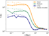 |
Fig. 5. Temperature profiles of short (Lf < 9 Mpc), medium-length (9 ≤ Lf < 20 Mpc), and long filaments (Lf ≥ 20 Mpc) in orange, green, and blue, respectively. The thick solid lines with circles correspond to the temperature profiles presented in Sect. 4.2, while the thin dotted lines with squares show the results in which contributions of galactic haloes are included (see Sect. 5). For each case, the horizontal grey lines represent the average temperatures of all the gas cells (CPmax points excluded) in the box. These profiles clearly show the isothermal cores of filaments. |
These temperature profiles exhibit the main feature of an isothermal core up to rcore = 1.5 Mpc from the axis of the filament. This trend is present in profiles of all three filament types (short, medium-length, and long). It is worth noting that the radial scale of rcore = 1.5 Mpc is independent of the resolution of the simulation, as shown in Appendix A. Most likely, a more fundamental physical reason is behind this characteristic scale (for example, an equilibrium between the gas pressure, volume, and density), but any conclusion is still premature at this stage and would require further investigations that go beyond the scope of the present paper. We note, however, that isothermal filament cores have already been observed in the temperature profiles of single simulated filaments in for example Klar & Mücket (2012) and Gheller & Vazza (2019); in this work we retrieve this property in a statistically significant way. We note that in the latter paper, the authors use an algorithm based on fixed density thresholds to detect filaments in the gas density field, which is a very different approach from the DisPerSE algorithm employed in this work.
Interestingly, we observe that the value of the plateau, Tcore, strongly depends on the length of the filament (e.g., orange vs. blue curves). For quantitative purposes, Table 3 reports the different values of Tcore, computed directly from the profiles as the average temperature of the points at r < 1.5 Mpc. On the left side of this table, we clearly see that cores of short filaments are more than three times hotter than those of long filaments. Indeed, the gravitational heating efficiency is likely stronger in the short population because of the deeper potential wells of these denser regions. This result is independent of the presence or the absence of galactic haloes, which is discussed in Sect. 5. We note that the temperature ranges of cores of filaments found in our analysis agree with the recent work of Tuominen et al. (2021), who studied filaments detected with the Bisous algorithm (Tempel et al. 2016) in the EAGLE simulation (Schaye et al. 2015).
Temperature Tcore and pressure Pcore at the cores of short (Lf < 9 Mpc), medium-length (9 ≤ Lf < 20 Mpc), and long filaments (Lf ≥ 20 Mpc).
At distances larger than r = 1.5 Mpc from the filament spine, the gas average temperature drops sharply. This drop is monotonic in short filaments, where the minimum of T ∼ 1.1 × 10⁵ K is reached in the most distant regions from the filament (> 50 Mpc). We emphasise that this value represents the average temperature in regions that are very far away from the spine, so gas from other structures (namely other, distant filaments) is included in this average. We checked that, by masking the gas cells from other filaments (at r ≤ 2 Mpc from the spine), we remove their contribution to the temperature and we find a lower background average, that is T ∼ 8.5 × 10⁴ K. Unlike for short filaments, the temperature profiles of the long filaments do not follow a monotonic trend. The long filaments exhibit a global minimum at r ∼ 10 Mpc, followed by a slight increase of the temperature, to finally reach the same background level as short (and medium-length) filaments. These dissimilarities between populations of short and long filaments at distances larger than r = 1.5 Mpc might come from their different environments in the cosmic web. Since short filaments statistically reside in denser regions (Galárraga-Espinosa et al. 2020), they are more likely to be closely surrounded by other dense structures (e.g., other filaments, clusters, or haloes) that contribute to the relatively high average temperature on the r > 1.5 Mpc outskirts. On the contrary, long filaments, tracers of less dense environments, extend into under-dense regions (voids) where the gas is cooler, which explains the dip at r ∼ 10 Mpc, before the temperature reaches the average value of the entire box. We note that these differences in temperature between short and long filaments closely reflect the phase portraits of Fig. 4.
We now split the different gas phases to see how their temperatures behave around filaments. We compute the temperature profiles of the five different phases, and we present these profiles in the panels of Fig. 6, where the same colour code as in Fig. 5 is adopted. In this section, we focus on the thick solid lines with circles and the thin dotted lines with squares are discussed in Sect. 5. We note that these profiles span a very broad total temperature range, from cold temperatures of T ∼ 104 K exhibited by the diffuse IGM (upper right panel), to the very hot values, of the order of T ∼ 2 × 10⁷ K, reached by the hot gas (lower right panel). This broad range simply reflects the definition of the gas phases.
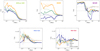 |
Fig. 6. Temperature profiles of the different gas phases (see Table 1), for short (Lf < 9 Mpc; orange curves), medium-length (9 ≤ Lf < 20 Mpc; green curves), and long filaments (Lf ≥ 20 Mpc; blue curves). The thick solid lines with circles correspond to the temperature profiles presented in Sect. 4.2, while the thin dotted lines with squares show the results in which contributions of galactic haloes are included (see Sect. 5). For each case, the horizontal grey lines represent the average temperatures of all the gas cells (CPmax points excluded) in the box. |
The temperature profiles of the five gas phases in Fig. 6 exhibit very different shapes and behaviours depending on the type of filament. All the gas phases around the short population show a rise in temperature from the outskirts to the core, except the hot gas that remains constant. The same trend is followed by gas around medium-length filaments, but in this case the temperature rise of the profile of WHIM is only very mild. Finally, the temperature profiles of the phases around long filaments exhibit a broader diversity.
The fact that the temperature profile of the hot gas phase remains essentially flat is easily understood by looking at Fig. 4, where the vast majority of the gas cells in filaments occupy only a limited and rather flat region that extends into the hot gas phase domain. Moreover, our results agree with recent findings from X-ray ROSAT observations. Tanimura et al. (2020a) detect a significant X-ray emission from hot gas at temperatures of  K (
K ( keV) in regions of cores of filaments, and this range is compatible with the mean temperature values of hot gas presented in this work.
To the contrary of all phases, diffuse IGM gas (upper right panel) exhibits the most significant temperature increase, from the background to the core of filaments. For example, cores of short filaments are up to seven times hotter than their background temperature. The increase of temperature from background to core is smaller in long filaments (for which the temperature is only multiplied by three), and this might be related to their location in less dense environments of the cosmic web (see Galárraga-Espinosa et al. 2020, and references therein). For all filaments, this significant temperature increase of the diffuse IGM profile may be due to the gravitational heating resulting from the accretion of this diffuse gas into the filament (as discussed in Sect. 3.1). We note that the maximum temperature is not higher than 105 K, given that beyond this threshold gas is counted as part of the WHIM phase.
Concerning the WHIM (middle left panel), we observe notably different temperature profiles for short, medium-length, and long filaments. The temperature of WHIM gas around short filaments increases with decreasing distance to the core, while in long filaments, the WHIM temperature shows a decrease on the outskirts (r ∼ 6−10 Mpc). Once again, this can be seen as a consequence of the different cosmic web environments of the short and long filaments. Gas accreted towards short filaments is likely rapidly heated by shocks, mergers, and feedback effects taking place in the denser environments that characterise these structures. On the contrary, gas falling into long filaments is probably not subject to the same dynamics (or perhaps simply with lesser efficiency) as gas falling into the short population.
Interestingly enough, the temperature profiles of the two phases corresponding to gas in and around haloes, halo gas and WCGM, respectively, do not appear to be sensitive to the different types of filaments (and therefore to the large-scale environment). As we move towards the spine, circumgalactic gas gets heated by shocks and feedback processes near galaxies in fairly the same way as for short and long filaments, as shown by their very similar profiles (see coloured curves in the WCGM and halo gas panels of Fig. 6). The profiles of these phases rather present a notable difference in the mean temperature levels (grey horizontal lines) whether galactic haloes are included into the temperature estimation or not. This feature is expected, given that halo gas and WCGM are tracers of haloes and that these collapsed structures can be located in background and foreground filaments, thus contributing to the rise of the mean temperature. Further details on the role that galactic haloes contribute to the temperature of filaments are discussed in Sect. 5.
4.3. Pressure profiles
We computed the profiles of gas pressure (see Sect. 2.4) around filaments using the same method as for temperature, described in Sect. 4.1. Before showing the results for each gas phase, we first focus on the general pressure profiles computed considering all the gas cells.
The latter are shown in Fig. 7 for short, medium-length, and long filaments. As expected from our previous results, filaments of different lengths have significantly different pressure profiles. At the core (r ≤ 1 Mpc) and on the outskirts (1 < r ≤ 10 Mpc), short filaments show values that are more than three times those of long filaments, as we reported on the left side of Table 3 (where the values correspond to the pressure read from the first radial bin). The same trends as for the temperature profiles of Fig. 5 are observed in Fig. 7; these trends are the monotonic decrease of short filament profiles and the presence of a global minimum in the pressure on the outskirts of long filaments. Again, these differences might be related to the different environments traced by the two populations (see text in Sect. 4.2). In comparison with the findings of Arnaud et al. (2010), who showed that pressure in the cores of galaxy clusters lies in the range of P = 1−300 × 10−3 keV.cm−3, we find that pressure in filaments, P = 4−12 × 10−7 keV.cm−3, is more than 1000 times smaller. This difference of three orders of magnitude is not surprising, given that the galaxy clusters are the densest and hottest structures of the cosmic web.
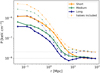 |
Fig. 7. Pressure profiles of short (Lf < 9 Mpc; orange curves), medium-length (9 ≤ Lf < 20 Mpc; green curves), and long filaments (Lf ≥ 20 Mpc; blue curves). The thick solid lines with circles correspond to the pressure profiles presented in Sect. 4.2, while the thin dotted lines with squares show the results in which contributions of galactic haloes are included (see Sect. 5). For each case, the horizontal grey lines represent the average pressures of all the gas cells (CPmax points excluded) in the box. |
Finally in Fig. 8, we show the pressure profiles of each gas phase. We note, as for the temperature, the very broad and particular pressure ranges of the different phases. Notably, the WCGM and hot phases reach maximum values of P ∼ 10−4 keV.cm−3, which are comparable to pressures on the outskirts of clusters of galaxies (Arnaud et al. 2010). We note that the pressure profiles of these phases, along with those of halo gas, do not show a strong dependence on the type of filament (i.e. the coloured curves are essentially the same), showing that the pressures of WCGM, halo, and hot gas are quite insensitive to the large-scale environment in the cosmic web, which is expected for phases that are associated with collapsed structures such as haloes. This is further discussed in Sect. 5. The opposite trend is observed in the pressure profiles of diffuse IGM and WHIM phases (first and second panels of Fig. 8). Indeed, they present significant differences for short, medium-length, and long filaments, showing that the properties of these phases are mainly ruled by the different environments in the cosmic web (traced by short and long filaments). This dependences were already pointed out by the diffuse IGM and WHIM temperature profiles of Fig. 6.
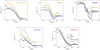 |
Fig. 8. Pressure profiles of the different gas phases (introduced in Sect. 2.5), for short (Lf < 9 Mpc; orange curves), medium-length (9 ≤ Lf < 20 Mpc; green curves), and long filaments (Lf ≥ 20 Mpc; blue curves). The pressure profiles in thick solid lines with circles are presented in Sect. 4.3, while the dotted lines with squares correspond to the results including galactic haloes (discussed in Sect. 5). The grey horizontal lines represent the average pressure of gas in each case. |
We now specifically focus on the WHIM phase (middle upper panel of Fig. 8), as some interesting features are exhibited by its pressure profiles. First, we note that WHIM pressures increase by almost two orders of magnitude from the outskirts to the cores of filaments. Almost all the profiles show a low-pressure zone at r ∼ 3 Mpc (with respect to the mean value), and this is most marked in the results of long filaments, which are tracers of cosmic regions with low and moderate densities. This dip was already visible in Figs. 5 and 7 and is probably due to the under-dense environment around the longer filaments, where the gas is cooler and less dense. This decrease of pressure happens at the same distance (r ∼ 3 Mpc) from the cores of all the filaments regardless of their length, exhibiting a characteristic radius of WHIM pressure around filaments. This common feature shows that WHIM gas might be subjected to the same physical processes (gravity and baryonic effects) in all types of filaments; although WHIM gas might not have the same efficiencies, since the pressure values are different. Moreover, WHIM gas pressure does not follow the distribution of galaxies: in the same simulations, we show that galaxies are statistically closer to cores of long filaments than to short, showing a characteristic radius of ∼3 and ∼5 Mpc, respectively (Galárraga-Espinosa et al. 2020).
5. Contribution of galactic haloes in filaments
All the above results present the properties of gas in the inter-filament medium, that is excluding the contribution of collapsed structures. In this section, we compare our above findings to those obtained when the galactic haloes (i.e. massive Mtot > 1012 M⊙ haloes containing at least one galaxy; see Sect. 2.3) are retained.
Figure 9 presents the phase-space of gas within 1 Mpc from the spine of filaments, including the contribution from gas in galactic haloes residing in these core regions. We note substantial differences in the filament contours with respect to those of Fig. 4. The contours are now in elliptical shapes that follow exactly those of galactic haloes towards the hottest and densest values at the boundaries between the WHIM, WCGM, and hot phases. The comparison of this phase-space to the first panel of Fig. 4 explicitly shows the contribution of gas associated with galactic haloes residing in filaments. We note that halo gas is also present in Fig. 9, with essentially the same significance as in Fig. 4, meaning that this phase cannot be interpreted as a contribution from massive galactic haloes (see Sect. 3.2).
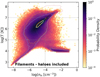 |
Fig. 9. Phase-space of gas in filaments, including the contribution of galactic haloes (i.e. haloes of mass Mtot > 1012 M⊙ hosting at least one galaxy of mass 109 ≤ M∗[M⊙] ≤ 1012). The 68% and 99% contours correspond to results of short (orange) and long filaments (blue), to galactic haloes (dotted green lines), and gas around the maximum density critical points of the field (CPmax, in dash-dotted red contours). |
The contribution of galactic haloes on the temperature profiles of filaments (thin dotted lines with squares in Fig. 6) is a general rise of the temperature at the core. We report these core temperature values in the right side of Table 3, which shows that the cores of filaments appear on average ∼1.2 times hotter when gas in haloes is included in the computation. This rise is expected as we have seen, in the phase-spaces of Figs. 4 and 9, that galactic haloes (statistically located in cores of filaments) contribute hotter and denser gas.
Regarding pressure, shapes, and amplitudes of the total profiles of Fig. 7, they seem to be extremely sensitive to the presence of galactic haloes in filaments. The values at the filament cores including galactic haloes are also reported on the right side of Table 3 and happen to be more than three times larger than core pressures when haloes are removed. These differences are not surprising, since galactic haloes and clusters are known to reach pressures that are several orders of magnitude higher (∼1000, see e.g., Arnaud et al. 2010) than our findings in the intra-filament medium, thus raising the average values.
We also disentangle the contributions of galactic haloes in the pressure and temperature profiles of each of the five different gas phases (see thin dotted lines with squares in Figs. 6 and 8). For the WHIM, WCGM, halo, and hot gas, we see that their values of temperature and pressure are clearly sensitive to the presence of galactic haloes, as solid and dotted profiles are significantly different both in temperature and pressure (see Figs. 6 and 8). The inverse trends are shown by the diffuse IGM phase. Its properties are dominated by the large-scale environment of short and long filaments, but the temperature and pressure profiles of the diffuse IGM phase are essentially the same whether galactic haloes are included or not, which simply reflects that this phase is absent in galactic haloes.
6. Sunyaev-Zel’dovich signal of filaments
Gas pressure can be measured via the thermal Sunyaev-Zel’dovich (SZ) effect (Zeldovich & Sunyaev 1969; Sunyaev & Zeldovich 1970, 1972). We therefore computed, from the mean pressure profiles of Fig. 7, the Compton y-profiles of gas around filaments. We present two extreme cases of filament orientation with respect to the line of sight (l.o.s.): the filament is perpendicular to the l.o.s., which gives a lower limit of SZ signal; and the filament is parallel to the l.o.s. (upper limit of SZ signal). In the following, we assume that filaments are far enough from the observer for all l.o.s. to be parallel.
For the perpendicular orientation, we computed the Compton-y value at the distance R from the spine of the filament (R is the projected distance on the sky) using the following equation:
 (8)
(8)
where σT, me, and c are the Thomson scattering cross-section, electron mass, and speed of light in vacuum, P is the mean pressure profile of Fig. 7, and l denotes the distance from the filament to the observer along the l.o.s..
In the second case, the filament is parallel to the l.o.s. and the Compton-y parameter depends on filament length Lf, as shown by
 (9)
(9)
Given that we deal with mean profiles of each filament population, the filament length values that we use are the average lengths  and 27.1 Mpc for short, medium-length, and long filaments, respectively.
The resulting Compton-y profiles are shown in Fig. 10 for short (left panel), medium-length (middle), and long filaments (right panel). The curves corresponding to the lower and upper signal limits are computed with Eqs. (8) and (9), respectively, and so the expected SZ signal from the various orientations should be bracketed between these curves in the colour-filled regions. The dark colours show the results from inter-filament gas excluding galactic haloes, while light colours correspond to the results including the contributions of these structures (as in Sect. 5).
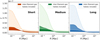 |
Fig. 10. Compton-y profiles of short (Lf < 9 Mpc), medium-length (9 ≤ Lf < 20 Mpc), and long filaments (Lf ≥ 20 Mpc) in the left, middle, and right panels, respectively. The dark colours show the SZ signal from inter-filament gas, that is gas that excludes the contribution of galactic haloes (massive Mtot > 1012 M⊙ haloes hosting at least one galaxy of stellar mass 109 ≤ M∗ ≤ 1012 M⊙). The light colours correspond to the SZ signal in filaments, where the contributions of galactic haloes are included. The lower and upper limits are computed with Eqs. (8) and (9), respectively, using the mean filament lengths of each population: |

At cores of filaments, we see that the values of the SZ signal for the perpendicular orientation are the largest in short filaments. This is due to the high pressures and the wider shape of the pressure profile of this population with respect to the other medium-length and long filaments. Concerning the parallel orientation, in the case in which the contribution from galactic haloes is removed (dark colours), the maximum SZ signal of the inter-filament medium is associated with long filaments, with y = 4.1 × 10⁻⁸ at their core (see dark blue upper limit), as expected from a signal that is proportional to filament length (Eq. (9)). Interestingly, we note that the upper values in cores of short and medium-length filaments, y ∼ 2−3 × 10⁻⁸, are close to that of the long-filament population; this is a result of the larger pressure values of these populations (see Fig. 7), which compensate the smaller filament lengths.
We note that the inclusion of gas in galactic haloes (light colours) increases significantly, by a factor three, the SZ signal, which is expected since these structures are hotter and denser and might be strong SZ sources by themselves. Indeed, when galactic haloes are taken into account, the resulting SZ signal at filament cores is around y ∼ 1.2 × 10⁻⁷ for the short population, y ∼ 1.5 × 10⁻⁷ for medium-length, and y ∼ 1.4 × 10⁻⁷ in long filaments. Maximum values are proportional to both pressure and filament length, so the similar y values in medium-length and long filaments are due to the higher pressures in the former, and to the longer lengths of the latter.
The SZ signal between pairs of clusters has been measured in Planck data, but the comparison of these results to our findings from simulations faces intrinsic limitations (e.g., instrumental noise, density of sources, foregrounds, etc.). It is however remarkable that our ranges of expected y values from filaments including haloes are of the same order of magnitude as SZ measurements around luminous red galaxies of mass M* > 1011.3 M⊙ (Tanimura et al. 2019). We also compare our results with the measured SZ signal from the bridge between the clusters A399-A401 of Bonjean et al. (2018). The signal in this filament was found to be remarkably high, with a value of the Compton-y parameter of ∼10−5. This is about two orders of magnitude higher than our predicted ranges in filaments (including the contribution of haloes), which is not surprising from this exceptional bridge.
We finally perform a more complete comparison with the recent measurements at 4.4σ significance of SZ signal from hot ionised gas around large-scale filaments presented in Tanimura et al. (2020b). In that paper, the authors built an average Compton-y profile by stacking the Planck 2015 (Planck Collaboration XXII 2016) y map, after removing the contribution of known groups and clusters, around filaments detected in the Sloan Digital Sky Survey (SDSS) by Malavasi et al. (2020). To reproduce the observational constraints of Tanimura et al. (2020b), we used the mean y profile we obtained for the long filament population. This is the closest possible to the sample of long (30−100 Mpc) filaments used in Tanimura et al. (2020b). We note that within the DisPerSE framework, filament lengths strongly depend on the density of tracers. The filament catalogue in Malavasi et al. (2020), from SDSS, and in our work are derived with 4 × 10⁻⁴ and 10−2 galaxy Mpc−3 respectively. As a consequence, the filament length distribution of the SDSS catalogue misses a lot of short filaments and thus peaks at 20−30 Mpc. We rescaled our mean y profile of long filaments to the average redshift of z = 0.4 of the observed filament sample. We also convolved the y profile by a Gaussian beam of 10 arcmin at redshift z = 0.4, corresponding to resolution of the SZ Planck map analysed in Tanimura et al. (2020b). Finally, following their approach, we computed the excess of SZ signal Δy with respect to the background by dividing the y profile derived from simulations by its background value, defined as the mean value at distances r > 25 Mpc from the spine.
The resulting Δy profiles are shown in Fig. 11 in light and dark purple, while the measurement from Tanimura et al. (2020b) is shown in grey (lines and shaded regions of 1σ errors). For the inter-filament gas, we find that the maximum SZ signal derived from the IllustrisTNG simulation is expected to be Δy = 2.6 × 10⁻⁸, which is compatible within the 1σ with the Tanimura et al. (2020b) profile. Given that our values correspond to upper bounds and that the observed filaments have a distribution of orientations, we deduce that a small contribution from the galactic haloes is expected in the measured signal, as suggested by the predicted signal of filaments including haloes (light purple curve) peaking at Δy = 8.0 × 10⁻⁸. Moreover, we note that the differences in the radial extent of the profiles could be explained by the reduced number of tracers in the SDSS catalogue (as mentioned above). The low galaxy density increases the uncertainties on the position of the filament spines, thus broadening the cores of the DisPerSE filaments (as shown in Galárraga-Espinosa et al. 2020). However at this stage, we are not able to distinguish this effect from possible thicker filament cores that would be expected at higher redshifts.
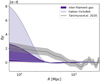 |
Fig. 11. Mean Δy profile of long filaments (Lf ≥ 20 Mpc), convolved with the Planck beam at z = 0.4. The dark purple shows the results of gas in the inter-filament medium (i.e. excluding the contribution of galactic haloes), while light purple presents our findings when galactic haloes are included. The lower and upper boundaries (solid purple lines) are computed using Eqs. (8) and (9), respectively. We compare our results from simulations with observations from Tanimura et al. (2020b), which are shown in grey (line and 1σ errors). |
7. Conclusions
Using the TNG300-1 simulation at redshift z = 0, we analysed the gas distribution and properties around the filamentary structures of the cosmic web. We distinguished five different gas phases, according to their density and temperature in the phase diagram, and we analysed their distribution around three different filament populations characterised by their length. The main results of this work are listed in the following.
– We find that cores of filaments (r ≤ 1 Mpc) essentially contain WHIM gas, but the hotter and denser phases of hot gas and WCGM are also significantly present (see Fig. 3 and Table 2). However, cores of short and long filaments are not made of exactly the same gas. Short filaments contain hotter gas than the long population, and long filaments possess a contribution of cold and diffuse IGM gas at their cores, that is absent in the short filament population (see phase-space of Fig. 4). These differences can be explained by the different large-scale environments, which are denser and less-dense for short and long filaments, respectively.
– We find that at r ∼ 1 Mpc from the spine of filaments WHIM gas completely dominates (> 80%) the entire baryon budget and the other phases are negligible. The different gas content at the cores and on the outskirts of filaments suggests that, apart from gravitational interactions, additional baryonic processes (whose efficiencies depend on the type of filament) affect the gas located at the cores, making it significantly different from the gas located further away from the spine. These additional baryonic processes might be due to the enhanced presence of haloes in these regions (Galárraga-Espinosa et al. 2020), which can accrete gas to their gravitational potential well, but also expel it by other feedback effects.
– We estimate that the average temperature and pressure at cores of filaments (r ≤ 1 Mpc) are T = 4−13 × 105 K, and P = 4−12 × 10−7 keV.cm−3, depending on the cosmic environment (see Table 3). Short filaments (living in denser regions) have temperature and pressure values that are three times those of the long population (which traces less-dense environments). All filaments present isothermal cores up to distances of rcore = 1.5 Mpc (see Fig. 5), which agrees with previous studies (Klar & Mücket 2012; Gheller & Vazza 2019). Finally, we observe that pressures in filament cores are ∼1000 times lower than those in cores of clusters.
– We estimate the SZ signal associated with gas in filaments and we find this signal in the range y = 0.5−4.1 × 10⁻⁸, depending on the type of filament (see Fig. 10). When gas from galactic haloes is included, the expected SZ signal increases significantly. In this case, the Compton-y parameter is in the range y = 0.1−1.5 × 10⁻⁷. We compare with the recent observations of gas in filaments (Bonjean et al. 2018; Tanimura et al. 2019, 2020b) and we find compatible SZ ranges with the expected signal of gas (Fig. 11).
– We show that diffuse phases (diffuse IGM and WHIM) are extremely sensitive to the large-scale cosmic environment, traced by short and long filaments (see their corresponding profiles in Figs. 6 and 8). On the outskirts of filaments (r > 1 Mpc) where these phases are the most present, there are statistically less haloes than in filament cores (Galárraga-Espinosa et al. 2020). Therefore, gas in these rather empty regions might be mainly shaped by the gravitational pull towards the denser regions of the cosmic web. Gravity is thus probably the main responsible for the rise of temperature of the accreted diffuse IGM (see Fig. 6), which is therefore converted into WHIM gas (Fig. 3) when approaching the spine of the filament. On the contrary, we find that the hotter and denser phases (WCGM, halo and hot gas) are almost insensitive to the global environment of short and long filaments. Given that these phases are associated with haloes (Fig. 4), their properties might be rather shaped by smaller scales (e.g., accretion onto haloes and halo mergers) and by galactic physics (e.g., feedback effects). Moreover, haloes are (biased) tracers of the density field and they are thus widely present in cores of filaments (Galárraga-Espinosa et al. 2020). Accordingly, we find that all the gas phases at filament cores (r ≤ 1 Mpc) are significantly impacted by the higher number density of these collapsed structures (see Figs. 6 and 8).
The physics of gas in the cosmic web is complex, and since baryonic matter is the only component that can be directly observed, it is essential to characterise its distribution and properties. In this sense, this work allowed us to build a clearer picture of the physical state of gas at any distance from the spine of filaments, and to identify more precisely the scales at which the different processes that shape gas in the cosmic web enter the game. Of course, further studies of the dynamics of gas and its evolution across redshifts are necessary to have a comprehensive understanding of the properties of gas in filaments, including dedicated mapping of the balance of power between the processes at play as function of time and environment in the cosmic web.
We note that the hydrogen number density is a direct tracer of the total gas mass density ρcell, as nH = XH ρcell/mp.
Acknowledgments
The authors thank the anonymous referee for helpful comments. This research has been supported by the funding for the ByoPiC project from the European Research Council (ERC) under the European Union’s Horizon 2020 research and innovation program grant agreement ERC-2015-AdG 695561. (ByoPiC, https://byopic.eu). The authors acknowledge the very useful comments and discussions with all the members of the ByoPiC team (https://byopic.eu/team/), and thank Marius Cautun for providing constructive feedback. DGE is especially grateful to Victor Bonjean and Céline Gouin for stimulating discussions. We thank the IllustrisTNG team for making their data publicly available.
References
- Aragón-Calvo, M. A., Platen, E., van de Weygaert, R., & Szalay, A. S. 2010, ApJ, 723, 364 [NASA ADS] [CrossRef] [Google Scholar]
- Arnaud, M., Pratt, G. W., Piffaretti, R., et al. 2010, A&A, 517, A92 [NASA ADS] [CrossRef] [EDP Sciences] [Google Scholar]
- Bond, J. R., Kofman, L., & Pogosyan, D. 1996, Nature, 380, 603 [NASA ADS] [CrossRef] [Google Scholar]
- Bonjean, V., Aghanim, N., Salomé, P., Douspis, M., & Beelen, A. 2018, A&A, 609, A49 [NASA ADS] [CrossRef] [EDP Sciences] [Google Scholar]
- Bonjean, V., Aghanim, N., Douspis, M., Malavasi, N., & Tanimura, H. 2020, A&A, 638, A75 [CrossRef] [EDP Sciences] [Google Scholar]
- Bonnaire, T., Aghanim, N., Decelle, A., & Douspis, M. 2020, A&A, 637, A18 [NASA ADS] [CrossRef] [EDP Sciences] [Google Scholar]
- Brinchmann, J., Charlot, S., White, S. D. M., et al. 2004, MNRAS, 351, 1151 [NASA ADS] [CrossRef] [Google Scholar]
- Cautun, M., van de Weygaert, R., & Jones, B. J. T. 2013, MNRAS, 429, 1286 [NASA ADS] [CrossRef] [Google Scholar]
- Cautun, M., van de Weygaert, R., Jones, B. J. T., & Frenk, C. S. 2014, MNRAS, 441, 2923 [NASA ADS] [CrossRef] [Google Scholar]
- Cen, R., & Ostriker, J. P. 2006, ApJ, 650, 560 [NASA ADS] [CrossRef] [Google Scholar]
- Cui, W., Knebe, A., Yepes, G., et al. 2018, MNRAS, 473, 68 [NASA ADS] [CrossRef] [Google Scholar]
- Cui, W., Knebe, A., Libeskind, N. I., et al. 2019, MNRAS, 485, 2367 [Google Scholar]
- de Lapparent, V., Geller, M. J., & Huchra, J. P. 1986, ApJ, 302, L1 [Google Scholar]
- Galárraga-Espinosa, D., Aghanim, N., Langer, M., Gouin, C., & Malavasi, N. 2020, A&A, 641, A173 [EDP Sciences] [Google Scholar]
- Gheller, C., & Vazza, F. 2019, MNRAS, 486, 981 [NASA ADS] [CrossRef] [Google Scholar]
- Gheller, C., & Vazza, F. 2020, MNRAS, 494, 5603 [Google Scholar]
- Gheller, C., Vazza, F., Favre, J., & Brüggen, M. 2015, MNRAS, 453, 1164 [Google Scholar]
- Gheller, C., Vazza, F., Brüggen, M., et al. 2016, MNRAS, 462, 448 [NASA ADS] [CrossRef] [Google Scholar]
- Haider, M., Steinhauser, D., Vogelsberger, M., et al. 2016, MNRAS, 457, 3024 [Google Scholar]
- Klar, J. S., & Mücket, J. P. 2012, MNRAS, 423, 304 [NASA ADS] [CrossRef] [Google Scholar]
- Kraljic, K., Arnouts, S., Pichon, C., et al. 2018, MNRAS, 474, 547 [Google Scholar]
- Kraljic, K., Pichon, C., Dubois, Y., et al. 2019, MNRAS, 483, 3227 [NASA ADS] [CrossRef] [Google Scholar]
- Liao, S., & Gao, L. 2019, MNRAS, 485, 464 [Google Scholar]
- Libeskind, N. I., van de Weygaert, R., Cautun, M., et al. 2018, MNRAS, 473, 1195 [NASA ADS] [CrossRef] [Google Scholar]
- Malavasi, N., Arnouts, S., Vibert, D., et al. 2017, MNRAS, 465, 3817 [NASA ADS] [CrossRef] [EDP Sciences] [Google Scholar]
- Malavasi, N., Aghanim, N., Douspis, M., Tanimura, H., & Bonjean, V. 2020, A&A, 642, A19 [CrossRef] [EDP Sciences] [Google Scholar]
- Martizzi, D., Vogelsberger, M., Artale, M. C., et al. 2019, MNRAS, 486, 3766 [Google Scholar]
- Nelson, D., Springel, V., Pillepich, A., et al. 2019, Comput. Astrophys. Cosmol., 6, 2 [Google Scholar]
- Nevalainen, J., Tempel, E., Liivamägi, L. J., et al. 2015, A&A, 583, A142 [NASA ADS] [CrossRef] [EDP Sciences] [Google Scholar]
- Pakmor, R., Guillet, T., Pfrommer, C., et al. 2018, MNRAS, 481, 4410 [CrossRef] [Google Scholar]
- Pereyra, L. A., Sgró, M. A., Merchán, M. E., Stasyszyn, F. A., & Paz, D. J. 2020, MNRAS, 499, 4876 [Google Scholar]
- Pillepich, A., Springel, V., Nelson, D., et al. 2018, MNRAS, 473, 4077 [Google Scholar]
- Planck Collaboration XIII. 2016, A&A, 594, A13 [NASA ADS] [CrossRef] [EDP Sciences] [Google Scholar]
- Planck Collaboration XXII. 2016, A&A, 594, A22 [NASA ADS] [CrossRef] [EDP Sciences] [Google Scholar]
- Ramsøy, M., Slyz, A., Devriendt, J., Laigle, C., & Dubois, Y. 2021, MNRAS, 502, 351 [Google Scholar]
- Schaap, W. E., & van de Weygaert, R. 2000, A&A, 363, L29 [Google Scholar]
- Schaye, J., Crain, R. A., Bower, R. G., et al. 2015, MNRAS, 446, 521 [Google Scholar]
- Shull, J. M., Smith, B. D., & Danforth, C. W. 2012, ApJ, 759, 23 [NASA ADS] [CrossRef] [Google Scholar]
- Singh, A., Mahajan, S., & Bagla, J. S. 2020, MNRAS, 497, 2265 [Google Scholar]
- Sousbie, T. 2011, MNRAS, 414, 350 [NASA ADS] [CrossRef] [Google Scholar]
- Sousbie, T., Pichon, C., & Kawahara, H. 2011, MNRAS, 414, 384 [NASA ADS] [CrossRef] [Google Scholar]
- Springel, V. 2010, MNRAS, 401, 791 [NASA ADS] [CrossRef] [Google Scholar]
- Springel, V., & Hernquist, L. 2003, MNRAS, 339, 289 [Google Scholar]
- Sunyaev, R. A., & Zeldovich, Y. B. 1970, Ap&SS, 7, 3 [NASA ADS] [Google Scholar]
- Sunyaev, R. A., & Zeldovich, Y. B. 1972, Comm. Astrophys. Space Phys., 4, 173 [Google Scholar]
- Tanimura, H., Hinshaw, G., McCarthy, I. G., et al. 2019, MNRAS, 483, 223 [Google Scholar]
- Tanimura, H., Aghanim, N., Kolodzig, A., Douspis, M., & Malavasi, N. 2020a, A&A, 643, L2 [EDP Sciences] [Google Scholar]
- Tanimura, H., Aghanim, N., Bonjean, V., Malavasi, N., & Douspis, M. 2020b, A&A, 637, A41 [CrossRef] [EDP Sciences] [Google Scholar]
- Taylor, E. N., Hopkins, A. M., Baldry, I. K., et al. 2011, MNRAS, 418, 1587 [NASA ADS] [CrossRef] [Google Scholar]
- Tempel, E., Stoica, R. S., Kipper, R., & Saar, E. 2016, Astron. Comput., 16, 17 [NASA ADS] [CrossRef] [Google Scholar]
- Tuominen, T., Nevalainen, J., Tempel, E., et al. 2021, A&A, 646, A156 [EDP Sciences] [Google Scholar]
- Ursino, E., Galeazzi, M., & Roncarelli, M. 2010, ApJ, 721, 46 [NASA ADS] [CrossRef] [Google Scholar]
- Valageas, P., Schaeffer, R., & Silk, J. 2003, MNRAS, 344, 53 [NASA ADS] [CrossRef] [Google Scholar]
- van de Weygaert, R., & Schaap, W. 2009, in The Cosmic Web: Geometric Analysis, eds. V. J. Martínez, E. Saar, E. Martínez-González, & M. J. Pons-Bordería, 665, 291 [NASA ADS] [Google Scholar]
- Weinberger, R., Springel, V., & Pakmor, R. 2020, ApJS, 248, 32 [Google Scholar]
- Zeldovich, Y. B., & Sunyaev, R. A. 1969, Ap&SS, 4, 301 [NASA ADS] [CrossRef] [Google Scholar]
Appendix A: Impact of the resolution of simulation
We study the effects of resolution on our results by performing the same analysis on the TNG300-2 simulation box. This box is the medium resolution run of the TNG300 series. Therefore, this box has the same characteristics as our baseline, the TNG300-1 simulation, except for a mass resolution (mDM = 3.2 × 10⁸ M⊙/h) that is eight times lower, a target baryon mass of mbaryon = 5.9 × 10⁷ M⊙/h, and a reduced number of gas cells Ngas = 12503.
Figure A.1 presents our findings concerning the mass fractions profiles φi of the different gas phases in these two simulations. The results of the reference TNG300-1 simulation (previously shown in Fig. 3) are presented in thin solid lines, and we compare these reference results to the φi profiles from the TNG300-2 box (in thick dashed lines). The profiles of TNG300-1 and TNG300-2 are quite similar, except for a very slight difference in the φi amplitudes that is the most noticeable at the core of filaments (r ≤ 1 Mpc). This difference is explained by the coarser Voronoi grid of the TNG300-2 box. Indeed, Fig. A.2 clearly shows that the distribution of the cell volumes in the TNG300-2 simulation is considerably shifted towards the larger values with respect to the TNG300-1 distributions, and this is the case for all the gas phases. As a consequence, the coarser grid of the TNG300-2 box leads to a slightly different distribution of the gas cells in the phase-space plane, meaning that, unsurprisingly, the classification of the gas cells into the different phases is less precise in this simulation.
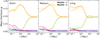 |
Fig. A.1. Gas mass fraction profiles φi (see Eq. (4)) of the five different gas phases in the TNG300-2 simulation (thick dashed lines), and in the reference TNG300-1 box (thin solid lines, same as Fig. 3). The colour codes follow those of Fig. 3, so that diffuse IGM, WHIM, WCGM, halo, and hot gas correspond to the green, yellow, purple, blue, and red curves, respectively. |
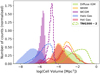 |
Fig. A.2. Distribution of the volumes of the gas cells in the TNG300-1 box (colour-filled histograms) and in the TNG300-2 simulation (dashed lines). The different colours correspond to the different gas phases considered in this work. |
For quantitative purposes, we show in Table A.1 the total fractions of the five different gas phases in our two simulations; we consider the full simulation boxes, excluding nodes and haloes. This table shows that the TNG300-2 box possesses slightly different fractions of cells with respect to the reference TNG300-1, with larger fractions in the hotter phases (e.g., hot gas and WHIM), and reduced fractions in the cooler phases (e.g., diffuse IGM, halo gas). As expected, this is reflected in the phase-space of gas at cores of filaments (r ≤ 1 Mpc) that we present in Fig. A.3. Here, the contours of the TNG300-2 simulation corresponding to the gas content of short and long filaments are slightly shifted in comparison to those of TNG300-1. Nevertheless, all the differences described above remain very tiny.
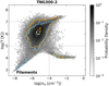 |
Fig. A.3. Phase-space diagram of cells at cores of filaments (r ≤ 1 Mpc) in the TNG300-2 simulation. The specific contours of short and long filaments are shown by the thick dashed lines in orange and blue, respectively. The results from TNG300-1 (presented in Fig. 4) are over-plotted in thin solid lines. |
Fractions of cells in the five different gas phases considered in this work for the full TNG300-1 and TNG300-2 simulations.
We now investigate the effects of resolution in the filament temperature and pressure profiles. We compare in Fig. A.4 the profiles of the TNG300-2 filaments to those of the reference TNG300-1 skeleton. Again, we observe only minor differences, which consist mainly in slightly hotter profiles and higher pressure values in the TNG300-2 curves. This only reflects the previously discussed features, which arise from the coarser Voronoi grid of the TNG300-2 simulation.
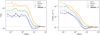 |
Fig. A.4. Temperature and pressure profiles of short, medium-length, and long filaments in the TNG300-1 and TNG300-2 simulations in thin solid and thick dashed lines, respectively. The results from TNG300-1 are the same as presented in Figs. 5 and 7. |
It is important to note that the characteristic radial scales of gas around filaments that we have discussed in the main text are found to be resolution independent, since all the results from the TNG300-1 and TNG300-2 simulations exhibit the same radial features, that is maximum of WHIM at r ∼ 1 Mpc and isothermal cores up to r ∼ 1.5 Mpc (see Sects. 3.1 and 4.2), despite the TNG300-2 box having a resolution that is eight times lower than the reference. Therefore, this study shows that the resolution of the simulation has only minor effects in the gas distribution and properties around cosmic filaments, as expected, since we focus in this work on the largest scales of the Universe. The main conclusions presented in this paper are therefore free from resolution effects.
All Tables
Mass fractions φi of the different gas phases at the core of short, medium-length, and long filaments.
Temperature Tcore and pressure Pcore at the cores of short (Lf < 9 Mpc), medium-length (9 ≤ Lf < 20 Mpc), and long filaments (Lf ≥ 20 Mpc).
Fractions of cells in the five different gas phases considered in this work for the full TNG300-1 and TNG300-2 simulations.
All Figures
|
Fig. 1. Two-dimensional projection of a slice of thickness 50 Mpc in the xy plane of the TNG300-1 box. The red points correspond to gas cells within the R200 radii of nodes (traced in this work by the DisPerSE maximum density critical points, see Sect. 2.3). The blue points represent gas around filaments, at distances closer than 1 Mpc from the spine of the cosmic web. Finally, the green points show gas in the R200 region of galactic haloes (i.e. within spheres of radius 1 × R200). The galactic haloes residing in filaments are clearly apparent (green over blue regions). The centres of the cells are plotted as points, but the TNG300-1 simulation is described by Voronoi cells having various volumes. |
| In the text | |
|
Fig. 2. Phase-space of the gas cells in the TNG300-1 simulation, shown by the normalised 2D histogram of the cells. The five different gas phases studied in this work are delimited by the thick dashed lines. They are defined as in Martizzi et al. (2019), and presented in Table 1 and Sect. 2.5. |
| In the text | |
|
Fig. 3. Gas mass fraction profiles φi (see Eq. (4)) of the five different phases (labelled by the index i) around short (left panel), medium-length (centre), and long filaments (right panel). All the gas phases used in this work are presented in Sect. 2.5. |
| In the text | |
|
Fig. 4. Phase portraits of gas, presenting the normalised 2D histograms of the gas cells in the corresponding structures. First panel: gas in filaments (within 1 Mpc from the core). Second panel: gas within the R200 radius of galactic haloes (defined as haloes of mass Mtot > 1012 M⊙ hosting at least one galaxy of mass 109 ≤ M∗[M⊙] ≤ 1012). Third panel: gas within the R200 radius of the DisPerSE maximum density critical points (CPmax), tracers of nodes. The 68% and 99% contours correspond to results of short (orange) and long filaments (blue), to galactic haloes (dotted green lines), and CPmax (dash-dotted red contours). |
| In the text | |
|
Fig. 5. Temperature profiles of short (Lf < 9 Mpc), medium-length (9 ≤ Lf < 20 Mpc), and long filaments (Lf ≥ 20 Mpc) in orange, green, and blue, respectively. The thick solid lines with circles correspond to the temperature profiles presented in Sect. 4.2, while the thin dotted lines with squares show the results in which contributions of galactic haloes are included (see Sect. 5). For each case, the horizontal grey lines represent the average temperatures of all the gas cells (CPmax points excluded) in the box. These profiles clearly show the isothermal cores of filaments. |
| In the text | |
|
Fig. 6. Temperature profiles of the different gas phases (see Table 1), for short (Lf < 9 Mpc; orange curves), medium-length (9 ≤ Lf < 20 Mpc; green curves), and long filaments (Lf ≥ 20 Mpc; blue curves). The thick solid lines with circles correspond to the temperature profiles presented in Sect. 4.2, while the thin dotted lines with squares show the results in which contributions of galactic haloes are included (see Sect. 5). For each case, the horizontal grey lines represent the average temperatures of all the gas cells (CPmax points excluded) in the box. |
| In the text | |
|
Fig. 7. Pressure profiles of short (Lf < 9 Mpc; orange curves), medium-length (9 ≤ Lf < 20 Mpc; green curves), and long filaments (Lf ≥ 20 Mpc; blue curves). The thick solid lines with circles correspond to the pressure profiles presented in Sect. 4.2, while the thin dotted lines with squares show the results in which contributions of galactic haloes are included (see Sect. 5). For each case, the horizontal grey lines represent the average pressures of all the gas cells (CPmax points excluded) in the box. |
| In the text | |
|
Fig. 8. Pressure profiles of the different gas phases (introduced in Sect. 2.5), for short (Lf < 9 Mpc; orange curves), medium-length (9 ≤ Lf < 20 Mpc; green curves), and long filaments (Lf ≥ 20 Mpc; blue curves). The pressure profiles in thick solid lines with circles are presented in Sect. 4.3, while the dotted lines with squares correspond to the results including galactic haloes (discussed in Sect. 5). The grey horizontal lines represent the average pressure of gas in each case. |
| In the text | |
|
Fig. 9. Phase-space of gas in filaments, including the contribution of galactic haloes (i.e. haloes of mass Mtot > 1012 M⊙ hosting at least one galaxy of mass 109 ≤ M∗[M⊙] ≤ 1012). The 68% and 99% contours correspond to results of short (orange) and long filaments (blue), to galactic haloes (dotted green lines), and gas around the maximum density critical points of the field (CPmax, in dash-dotted red contours). |
| In the text | |
|
Fig. 10. Compton-y profiles of short (Lf < 9 Mpc), medium-length (9 ≤ Lf < 20 Mpc), and long filaments (Lf ≥ 20 Mpc) in the left, middle, and right panels, respectively. The dark colours show the SZ signal from inter-filament gas, that is gas that excludes the contribution of galactic haloes (massive Mtot > 1012 M⊙ haloes hosting at least one galaxy of stellar mass 109 ≤ M∗ ≤ 1012 M⊙). The light colours correspond to the SZ signal in filaments, where the contributions of galactic haloes are included. The lower and upper limits are computed with Eqs. (8) and (9), respectively, using the mean filament lengths of each population: |
| In the text | |
|
Fig. 11. Mean Δy profile of long filaments (Lf ≥ 20 Mpc), convolved with the Planck beam at z = 0.4. The dark purple shows the results of gas in the inter-filament medium (i.e. excluding the contribution of galactic haloes), while light purple presents our findings when galactic haloes are included. The lower and upper boundaries (solid purple lines) are computed using Eqs. (8) and (9), respectively. We compare our results from simulations with observations from Tanimura et al. (2020b), which are shown in grey (line and 1σ errors). |
| In the text | |
|
Fig. A.1. Gas mass fraction profiles φi (see Eq. (4)) of the five different gas phases in the TNG300-2 simulation (thick dashed lines), and in the reference TNG300-1 box (thin solid lines, same as Fig. 3). The colour codes follow those of Fig. 3, so that diffuse IGM, WHIM, WCGM, halo, and hot gas correspond to the green, yellow, purple, blue, and red curves, respectively. |
| In the text | |
|
Fig. A.2. Distribution of the volumes of the gas cells in the TNG300-1 box (colour-filled histograms) and in the TNG300-2 simulation (dashed lines). The different colours correspond to the different gas phases considered in this work. |
| In the text | |
|
Fig. A.3. Phase-space diagram of cells at cores of filaments (r ≤ 1 Mpc) in the TNG300-2 simulation. The specific contours of short and long filaments are shown by the thick dashed lines in orange and blue, respectively. The results from TNG300-1 (presented in Fig. 4) are over-plotted in thin solid lines. |
| In the text | |
|
Fig. A.4. Temperature and pressure profiles of short, medium-length, and long filaments in the TNG300-1 and TNG300-2 simulations in thin solid and thick dashed lines, respectively. The results from TNG300-1 are the same as presented in Figs. 5 and 7. |
| In the text | |
Current usage metrics show cumulative count of Article Views (full-text article views including HTML views, PDF and ePub downloads, according to the available data) and Abstracts Views on Vision4Press platform.
Data correspond to usage on the plateform after 2015. The current usage metrics is available 48-96 hours after online publication and is updated daily on week days.
Initial download of the metrics may take a while.