| Issue |
A&A
Volume 649, May 2021
|
|
|---|---|---|
| Article Number | A132 | |
| Number of page(s) | 11 | |
| Section | Astronomical instrumentation | |
| DOI | https://doi.org/10.1051/0004-6361/202039629 | |
| Published online | 27 May 2021 | |
Monitoring precipitable water vapour in near real-time to correct near-infrared observations using satellite remote sensing
Center for Space and Habitability (CSH), University of Bern, Gesellschaftsstrasse 6, 3012 Bern, Switzerland
e-mail: This email address is being protected from spambots. You need JavaScript enabled to view it.
Received:
9
October
2020
Accepted:
5
March
2021
Abstract
Context. In the search for small exoplanets orbiting cool stars whose spectral energy distributions peak in the near infrared, the strong absorption of radiation in this region due to water vapour in the atmosphere is a particularly adverse effect for ground-based observations of cool stars.
Aims. To achieve the photometric precision required to detect exoplanets in the near infrared, it is necessary to mitigate the effect of variable precipitable water vapour (PWV) on radial-velocity and photometric measurements. The aim is to enable global PWV correction by monitoring the amount of precipitable water vapour at zenith and along the line of sight of any visible target.
Methods. We developed an open-source Python package that uses imagery data obtained with the Geostationary Operational Environmental Satellites (GOES), which provide temperature and relative humidity at different pressure levels to compute the near real-time PWV above any ground-based observatory that is covered by GOES every 5 min or 10 min, depending on the location.
Results. We computed PWV values on selected days above Cerro Paranal (Chile) and San Pedro Mártir (Mexico) to benchmark the procedure. We also simulated different pointing at test targets as observed from the sites to compute the PWV along the line of sight. To asses the accuracy of our method, we compared our results with the on-site radiometer measurements obtained from Cerro Paranal.
Conclusions. Our results show that our publicly available code proves to be a good supporting tool for measuring the local PWV for any ground-based facility within the GOES coverage, which will help to reduce correlated noise contributions in near-infrared ground-based observations that do not benefit from on-site PWV measurements.
Key words: infrared: stars / atmospheric effects / methods: observational / techniques: image processing
© ESO 2021
1. Introduction
In our search for potential habitable exoplanets, cool stars such as the TRAPPIST-1 system (Gillon et al. 2016; Luger et al. 2017) have proven to be promising candidates. In the past years, numerous detections of exoplanets have been reported, and projects such as SPECULOOS (Jehin et al. 2018; Delrez et al. 2018) aim to detect small exoplanets orbiting ultra-cool stars for which the spectral energy distribution peaks in the near infrared. A key requirement for detecting small exoplanets orbiting cool stars is to efficiently correct for the adverse effects induced by the Earth’s atmosphere. Water vapour is one of the main atmospheric gases that absorbs incoming radiation in the near infrared (NIR) region, specifically around 1 μm and 5 μm (see Peixoto & Oort 1992). This characteristic of water vapour poses a serious challenge for ground-based observations in the NIR region. The amount of precipitable water vapour is variable in space and time, thus inducing correlated noise in the photometric time-series, potentially masking or mimicking an exoplanet transit (Baker et al. 2017). In the search for exoplanets with the radial velocity (RV) method, telluric lines can limit the measurement accuracy at the level of 1 m s−1 (Cunha et al. 2014), which cannot be neglected for instruments aiming to achieve a precision better than m s−1, such as ESPRESSO (Pepe et al. 2021). These issues justify the interest in monitoring the temporal variability of precipitable water vapour (PWV) during observations to better understand and correct for correlated noise due to the atmosphere in the search for small planets.
Several studies (Kassomenos & McGregor 2006; Otárola et al. 2009; Buehler et al. 2012; Marín et al. 2015) have focused on monitoring and characterising precipitable water vapour variability from a meteorological point of view, for which daily, monthly, or seasonal values are of interest. Thus, the temporal resolution between measurements may be lower (e.g. retrieval of data every 12 or 24 h) than in studies with an astronomical focus. While the average PWV above certain locations is an important factor for astronomical site selection, a much higher temporal resolution of several minutes is required to study PWV variability over timescales relevant for RV or photometric exoplanet observations. In particular, the relevant timescales for photometric observations is the transit duration, which has been observed to last less than an hour for some exoplanets (see Gillon et al. 2017). Much effort has been put into mitigating the effect of water vapour absorption on astronomical observations. Baker et al. (2017) developed an automatic PWV monitoring multiband photometer system and installed it at the Fred Lawrence Whipple Observatory in Arizona. The instrumentation achieves a precision better than 0.5 mm for PWV conditions below 4 mm, and the data were compared to GPS monitoring systems. A GPS is commonly used to measure PWV by means of the delay of satellite signals, which can be formulated as an excess length and is usually determined at the zenith above the ground-based receiver station. This parameter, called zenith total delay (ZTD), includes a wet delay component, which is a function of the water vapour distribution (Mile et al. 2019). The issue of measuring PWV from GPS data arises on the uncertainty in the ZTD measurement because the standard deviation for PWV is approximately the same for all measurements. Therefore the relative uncertainty is high for low values of PWV, but low for high values of PWV (Buehler et al. 2012). The GPS method is therefore less accurate in dry conditions, which are typical of most astronomical observing sites. In this paper we define a region as dry for an average of PWV below 4 mm.
Additionally, Buehler et al. (2012) conducted a multi-instrument comparison of PWV over the subarctic site Kiruna (Sweden). The different sensors and retrieval methods used involved radiosondes, GPS, ground-based Fourier-transform infrared spectrometer, ground-based microwave radiometer, and satellite-based microwave radiometer. The available parameters for each measurement taken by the radiosonde included time of flight, pressure, temperature, relative humidity, height, and dew point, but measurements were limited to periods of scheduled launches. To estimate PWV using Fourier transform infrared spectroscopy, solar absorption spectra were recorded and processed via radiative transfer models, but this technique requires cloud-free conditions, and the measurements were limited to periods when the Sun was above the horizon. The ground-based radiometer measured thermal emission spectra to monitor stratospheric trace gases. To retrieve ozone profiles, the spectrum has to be corrected for varying tropospheric water vapour, resulting in an offset. Then models based on radiative transfer theory were used to calculate a water vapour profile matching the offset and actual temperature and pressure values. Finally, because the atmosphere is too dry in polar regions, the satellite-based radiometer measured the brightness temperature instead of relative humidity and related it with PWV. The results agreed reasonably well, differing by values below ±1 mm, except for ground-based measurements without filtering out cloud presence (Buehler et al. 2012). Additionally, given that the systematic differences depend strongly on the instrument, location, and method, it is not conclusive which technique is most suitable for estimating PWV. Additionally, the technique that is most suitable from a scientific point of view depends on practical factors such as maintenance costs.
Andre Erasmus conducted several studies on forecasting of precipitable water vapour in Chile. Erasmus & van Staden (2001) performed a survey using 58 months of meteorological satellite data taken every 12 h between July 1993 and September 1999 in Northern Chile to evaluate the best site for the Extremely Large Telescope (ELT) based on cloud cover and water vapour. This work concluded that Paranal, Quimal, Yacas, and Cascasco were the best candidates based on cloud cover. Cerro Chascón was found to be the best site based on PWV analysis. The ELT is now under construction on Cerro Armazones. Researchers have also made use of older GOES imagery to compute PWV values every 6 h (Erasmus & Sarazin 2002) or every 3 h (Marín et al. 2015) by means of radiance data. Planck functions relate radiance with brightness temperature, and the method to compute PWV involves a semi-empirical formula valid only for the 6.7 μm channel between 600 and 300 hPa pressure levels. We note that this approach is no longer valid using data of currently operational GOES satellites because these satellites are not equipped with a 6.7 μm channel. Instead, they take measurements at bands with central wavelength of 7.34, 6.93, and 6.17 μm. This allows measuring low- (from sea level to approximately 900 hPa), mid- (from approximately 900 to 700 hPa) and high-level (from 700 to 300 hPa) water vapour, respectively (NOAA 2019a).
Querel & Kerber (2014) used the Low Humidity and Temperature Profiling (LHATPRO) microwave radiometer, installed at the ESO Cerro Paranal observatory in support of the Very Large Telescope (VLT), to monitor the amount of PWV above the site down to an elevation angle of 27.5° every 6 h during a period of 21 months. They found that PWV across the sky over Paranal is very uniform, suggesting that constraining PWV measurements at the zenith would be sufficient to support most science applications. Another important result is that the highest spatial and temporal variation of PWV occurs for low PWV conditions. Finally, they recommend providing simultaneous line-of-sight observations pointed toward the target.
A Python package that estimates PWV was developed by Perrefort et al. (2018), which provides models for atmospheric transmission due to water vapour at Kitt Peak National Observatory, Arizona, or user-specified sites in the continental United States region and most of central America affiliated with the SuomiNet project1. Given a date and airmass, the package determines the PWV column density using data regarding the delay in GPS signals that is published every hour.
There is no defined boundary set to compute the PWV. While the total PWV value is computed between sea-level atmospheric pressure and approximately 100 hPa, this is not the ideal choice when the PWV is estimated on high-altitude sites because it does not take the actual pressure on the surface into account given that pressure decreases with height. Applying this definition at Cerro Paranal, where the mean surface pressure is 750 hPa, would lead to an overestimated PWV value due to contribution below this pressure level. Erasmus & van Rooyen (2006) set an upper limit of 300 hPa because at lower pressure, the contribution from PWV is very small (see Sect. 4.4). Marín et al. (2015) estimated the integrated PWV in the Chajnantor plateau (5100 m above sea level) in Chile for pressure levels from 550 hPa to 100 hPa because the mean surface pressures at the study sites ranged between 550 hPa and 500 hPa over the year, and the upper pressure level corresponds to the highest level available in the dataset they used.
The aim of the present study is to present fyodor2, an open-source Python package that uses GOES imagery data to compute the near real-time PWV at any site covered by the GOES-W/E (Americas). The main motivation is to assist data analyses of observations of cool stars in the NIR region, including the SAINT-EX Observatory (Demory et al. 2020) located in San Pedro Mártir (Baja California, Mexico). The novelty of our approach is that at the user’s request, the code computes the amount of precipitable water vapour at the zenith or along the line of sight to a target in the sky. To asses the program performance, ESO’s Cerro Paranal (Chile) Observatory was chosen to compare the results with the measurements obtained by the LHATPRO instrument at the same location.
2. Methodology
We present the instrumentation and methodology in this section. First, in Sects. 2.1 and 2.2 we introduce the currently operational satellites of the National Oceanic and Atmospheric Administration (NOAA) and the relevant data products with their range, accuracy, and performance. Then, Sect. 2.3 is dedicated to the coordinate system used by GOES satellites. In Sect. 2.4 we present the theoretical ground on the PWV, along with the complete derivation in Appendix A. Finally, the proposed method for computing the PWV along the line of sight to a target in the sky is explained in Sect. 2.5.
2.1. GOES-R series
NOAA currently operates two Geostationary Operational Environmental Satellites (GOES), at 75° west and 137° west longitude, to provide continuous weather imagery and monitoring of meteorological data across the USA and most part of the American continent. The current generation is called GOES-R series, and the primary instrument is the Advanced Baseline Imager (ABI), a multi-spectral channel, two-axis scanning radiometer that provides geolocated observations on three standard coverage regions: Full Disk, defined as a circle with 17.4° angular diameter from the perspective of the satellite covering a near hemispheric Earth region, CONUS covers an area of 10N–60N latitude and 60W–125W longitude, and Mesoscale, equivalent to a region of approximately 1000 × 1000 km. ABI Bands 1 to 6 measure the solar reflected radiance at visible and NIR wavelengths, while bands 7 to 16 measure the emitted radiance at infrared wavelengths. All data are made available in the netCDF-4 file format (NOAA 2019b). For this study we used data obtained by the GOES-16 satellite.
2.2. GOES-R data products
Among all data products provided by NOAA, which are publicly available for download3, we required only temperature, pressure, and relative humidity data to compute the PWV. The data products used are labeled Legacy Vertical Temperature Profile (LVTP) and Legacy Vertical Moisture Profile (LVMP), which make use of all infrared channels (Bands 7−16). Both data products contain a three-dimensional variable with pixel values identifying the air temperature and relative humidity at 101 discrete standard pressure levels. Each file corresponds to one measurement for all pressure levels, and the measurements are taken every 10 min for the Full Disk region and every 5 min for the continental United States (CONUS) region. Temperature values are provided in Kelvin, while relative humidity is given as a fraction ranging between 0 and 1. The spatial resolution of both data products is 10 km, and data are generated if the following criteria are met: (1) Clear sky and (2) Geolocated source data to local zenith angles of 80° for both daytime and nighttime conditions (angle between the line of sight to the satellite and the local zenith at the observation target).
The temperature range is between 180 and 320 K with an accuracy of 1 K and a precision of 2 K between the top of the boundary layer and 400 hPa. Regarding relative humidity, accuracy and precision are 0.18 from the surface up to 300 hPa and 0.2 between 300 and 100 hPa.
Conditions for good-quality data also require latitude |ℓ| ≤ 70° (NOAA 2019a). Before the data are released, internal algorithms check the data for their quality. If a pixel does not fulfil the conditions, the data point is masked. It is very important to note that of the temperature and moisture values taken at 101 pressure levels, only 54 temperature and 35 moisture pressure levels are actually measured. These temperature levels are from approximately 103 hPa to 1014 hPa, while the moisture levels are from 300 hPa to 1014 hPa. The remaining levels are retrieved by interpolation.
Additionally, NOAA offers a product containing the integrated column water vapour amount from the surface to a height corresponding to a pressure of 300 hPa called total precipitable water (TPW). It has an accuracy of 1 mm and precision of 3 mm. The advantages and disadvantages of using this end product are discussed in Sect. 4.
2.3. ABI fixed grid
The coordinate system used by the GOES-R, called advanced baseline imager (ABI) fixed grid, is a projection based on the viewing perspective of the location of the satellite in geostationary orbit. Data points at a particular horizontal spatial resolution on the fixed grid have the same angular separation from the satellite’s perspective. Depending on the data product resolution, Earth is covered by equally sized squares, each one of them populated by data. The x-axis represents the ABI east-west scan angle, and the y-axis represents the north-south scan angle. GOES-16 products with a spatial resolution of 10 km at nadir have data points with an angular separation of 280 μ radians. To locate a specific pixel in a file, the horizontal and vertical index have to be given. The dimension of a data product with 10 km horizontal resolution is 1086 × 1086.
To navigate through data points in the ABI fixed grid, a transformation between latitude and longitude coordinates and ABI fixed grid scan angle coordinates has to be performed. The equations presented here assume points lying on the Geodetic Reference System 1980 ellipsoid. Given geodetic latitude ϕ and longitude λ in radians, the scan angles x and y are computed by the following equations (NOAA 2019a):
 (1)
(1)
where sx is the x-axis from the satellites’ reference frame and is defined as the line from the satellite to the centre of the Earth, sy is the y-axis aligned with the equatorial axis and sz completes the orthogonal coordinate system and is parallel to the line that passes from the centre of the Earth to the north pole. These quantities are computed as follows:
 (2)
(2)
H is the satellite height from the centre of Earth in meters, λ0 is the satellite longitude, also called longitude of projection origin. These quantities, as well as Earth’s semi-major axis req, semi-minor axis rpol, and eccentricity e, are included in every GOES netCDF-4 file. The geocentric latitude ϕc and geocentric distance to the point on the ellipsoid rc are
 (3)
(3)
2.4. Definition of PWV
Among the variable gases, water vapour is predominant in the lower troposphere, comprising up to 4% of the volume of air in the atmosphere (Ahrens 2013). The amount of water vapour contained in a unit area column of air between two pressure levels is given by the expression (Kassomenos & McGregor 2006)
 (4)
(4)
where q is the specific humidity, p is the pressure, and g is the acceleration due to Earth’s gravity. It represents the amount of liquid water that would result if all the water vapour in the column were condensed and is usually expressed in units of kg m−2 or mm after dividing the expression above by the density of water ρw.
A negative sign has to be included in front of the integral if we define that for ascending index i = 1, 2, 3, …, the absolute value of the pressure decreases. This convention is adopted from now on because pressure decreases with increasing altitude.
The specific humidity can be expressed as a function of temperature, pressure, and relative humidity as follows (see Appendix A for the derivation and details):
 (5)
(5)
2.5. PWV along the line of sight to the target
In this section the novel method for computing the PWV along the line of sight to the target in the sky is described. Computing the PWV at the zenith is the easiest task because the values of temperature and relative humidity are found in the same coordinates on the GOES-R data files at all times, but estimating the PWV along the line of sight to the celestial target requires additional computation. The idea behind our procedure is to compute an inclined column along the line of sight to the target instead of doing so vertically above the location. Figure 1 illustrates this concept (note that the scales are exaggerated for better understanding). Let O be an observation point on Earth looking at an arbitrary target in the sky. Consider each pressure level as a circular shell concentric to Earth. The line of sight to the target intercepts the ith pressure layer Pi at a certain point. Now, if we connect this interception point with a straight line to the centre of the Earth, we obtain a point Li on the surface of the Earth, which gives us the projection of the point where the line of sight intercepts the ith pressure level. If a target is fixed at the zenith, then all projection points from all pressure levels are located at the location of the observation, but for any other location on the sky, the latitude and longitude coordinates of the projection points have to be computed in order to retrieve temperature and relative humidity data at each relevant pressure level.
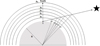 |
Fig. 1. Illustration of where the projection points Li are located. The PWV is estimated from the observer O along the line up to the pressure level Pn. |
To locate the projected places on Earth, the line of sight has to be specified from the point of observation. Horizontal celestial coordinates are best suited for this because the coordinates of a target are given by the altitude (also called elevation) angle α, azimuth δ, and time in the observation frame of reference (see Smart 1977). Assuming that the point of observation lies on a plane tangential to Earth’s surface, the projection point at a certain height can be computed with Pythagoras’ theorem in Euclidean geometry. This assumption of a flat surface is valid for the scales considered here. Estimating the PWV up to a pressure level of 300 hPa corresponds to a height of approximately 11 km. Constraining observations to elevation angles above 30°, the maximum projected distance is 19.05 km in Euclidean geometry, while the arc length in spherical geometry from the observation point to the projection point equals 18.97 km. The difference is about 81.64 m, which gives the maximum error by this method. Considering that the GOES-R spatial resolution is 10 km, this error is negligible, and thus assuming a flat surface is valid.
When the geodesic distance Δd to the observation point is computed, the azimuth angle is used to estimate the distance along longitude Δdlon and latitude Δdlat lines. Finally, the angle subtended from the centre of the Earth between the observation point and the projection point is computed for both latitude and longitude and then added to the coordinates of the observation point, which yields the coordinates of the projection point (latprojection and lonprojection). These coordinates are used to locate the temperature and relative humidity data on the GOES-R data files. All equations are listed below:
 (6)
(6)
 (7)
(7)
 (8)
(8)
 (9)
(9)
 (10)
(10)
where all angles are given in radians, REarth is the radius of Earth, and h is the height computed from the pressure via the barometric formula (see Eq. (11)).
3. PWV program
We present fyodor, a Python package for computing PWV above a location or along the line of sight for arbitrary astronomical sources from publicly available GOES-R data products. fyodor is built based on several open-source packages including python-netCDF4, NumPy (Harris et al. 2020), matplotlib (Hunter 2007), AstroPy (Astropy Collaboration 2013, 2018), astroplan (Morris et al. 2018), and bs4 (Richardson 2007). Here we describe the process from downloading the files until the retrieval of PWV. Each moisture and temperature file provided by NOAA has to be locally stored. Users can either search and request data on given dates and times, or they can create a subscription for delivery of specific GOES-R products. The user must download each file individually. The program works with GOES-16 and GOES-17 imaging data. For a complete day in the Full Disk region, a new file with data is available every 10 min, making a total of 144 files of temperature data and 144 files of moisture data. Each file has a size of approximately 240 MB, corresponding to 70 GB of data for a complete day. However, the GOES-R satellites take measurements of the CONUS region every 5 min, which doubles the amount of files but reduces the size of each one of them to 30 MB, equivalent to 17 GB for a complete day. If the user prefers to download TPW, each file for the Full Disk and CONUS region has a size of 1.4 MB and 0.28 MB, respectively, corresponding to 201.6 MB and 80 MB for a complete day, respectively.
The name of a typical GOES-R file contains the abbreviation of the product (in our case, LVMP, LVTP, and TPW), the region of observation (F for Full Disk and C for CONUS), satellite (G16 or G17) and the starting time of measurement in following order: year, number of day, hour, minutes, and seconds. Files obtained by a subscription have the number of processing order at the beginning of the name. Here we show an example with four files, two moisture and two temperature measurements. One of the files was retrieved via subscription for clarity on how the different steps of the program work.
3.1. download_nc(): Download the files
To avoid manually downloading each file, the download_nc function can be called. It takes three string arguments: the website provided by NOAA with the downloadable files, the directory where a new folder containing the files should be created, and the day on which the measurements were taken in the format “dd mm yyyy”:
Example 1. Download .nc files.
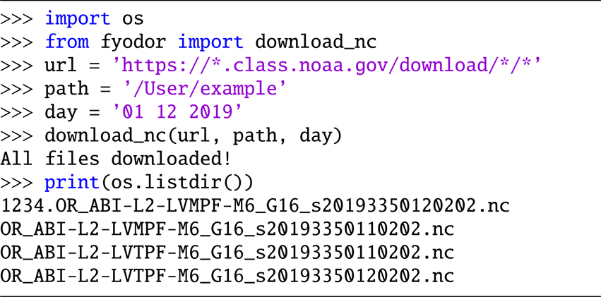
download_nc was developed specifically for the design of NOAA’s Comprehensive Large Array-data Stewardship System (CLASS) website, consisting of a table with every netCDF4 file requested by the user. As long as the NOAA CLASS website remains unchanged, the routine will work. The caveat of this method is that due to an occasional slow response by the website or slow internet connection, the script tends to time out and fail, forcing the user to run it again. It is worth mentioning that the code does not differentiate between files corresponding to the Full Disk and CONUS region. The user has to make sure to store the different datasets in separate folders.
3.2. rename_nc(): Rename subscription files
Because the name of each file contains the time of measurement, the files can be sorted in chronological order. However, data obtained from a subscription have the number of processing order at the beginning. If the file name is not renamed, sorting the files will not necessarily order them chronologically. To delete the first string of numbers of all files in a specific folder, we can call rename_nc, giving the directory as the argument:
Example 2. Rename .nc files.
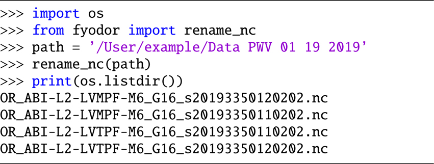
We note that the name of the first file was changed by removing the string “1234”.
3.3. pwv(): Compute PWV at the zenith
The package netCDF4 reads the files and lists all variables, ranges, and dimensions contained in the file. All necessary Earth parameters (such as the semi-major axis) are assigned here to variables by reading out just the first file in the folder.
Each file contains 101 standard pressure levels starting at 1100 hPa up to 0.005 hPa. These are the same for all GOES-16 products containing the pressure variable. For this reason, the script assigns the pressure variable just once out of the first file.
The data files contain time variables represented in seconds since J2000 epoch (2000-01-01 12:00:00 UTC). The script converts into human readable time in UTC format.
In order to compute the height as a function of pressure, hydrostatic balance in the atmosphere is assumed. The height depends on the pressure (P), the universal gas constant (R), acceleration due to Earth’s gravity (g), standard atmospheric pressure (P0), and a typical surface temperature (T0) of 288 K (Wells 2012). We also assume a constant lapse rate (L). The height has to be considered as an approximation, but it is necessary to compute the PWV along the line of sight to a target in the sky:
 (11)
(11)
Although the variation on gravitational acceleration and the gas constant are negligible from the surface to 300 hPa, the temperature changes considerably over space and time. The limitation of the formulation used in the code is that the reference temperature of 288 K is the same for any location for any time of the year.
The pwv function requires several arguments. As for all other objects, the directory containing the files is necessary. The observing location is required and accepts three different inputs: “Cerro Paranal”, “San Pedro Martir”, and “Other”. The first two automatically set the latitude and longitude for the Cerro Paranal or San Pedro Mártir observatory. Alternatively, “Other” gives the user the option to enter a valid value for latitude (between −81.3281 and 81.3281°) and longitude (between −156.2995 and 6.2995°), defined in the GOES-R documentation (NOAA 2019b). All relevant coordinates located on Earth are transformed into scan angles according to Eq. (1) with its auxiliary Eqs. (2) and (3).
Next, the function needs the pressure level boundaries. As we discussed in the Introduction, the contribution to PWV is very small above 300 hPa, therefore it is reasonable to set this as a cutoff. The lower boundary (in height) can be set to the standard atmospheric pressure, or ideally, the surface pressure at the location of interest. At Cerro Paranal, the mean atmospheric pressure on the surface is 750 hPa4, while in San Pedro Mártir, it is 727 hPa5.
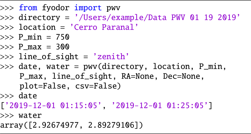
To compute the PWV above the location, we have to set the argument line_of_sight = ‘zenith’. Finally, plot = True displays a plot with the results and saves a .png figure in the directory, while csv = True generates and saves a .csv file with the time of measurement and PWV value. Below is a complete example at Cerro Paranal:
Example 3. Compute PWV above Cerro Paranal.
3.4. pwv(): Compute the PWV along the line of sight
Alternatively, to obtain the PWV along the line of sight to a target, we have to set line_of_sight = ‘target’. The coordinates of the target in equatorial coordinates have to be given. In Sect. 2.5 the equations were derived making use of horizontal celestial equations, but instead, the user is still asked to input right ascension (RA) and declination (Dec) values. The reason is that equatorial coordinates require less input information because RA and Dec are constant numbers (during a long period of time), and computationally, it is much easier to transform from RA and Dec into altitude and azimuth than typing these angles and time of measurement and then compute the angles for each time of measurement of the satellite (i.e. each data file). The astropy package carries out the transformation and assigns the altitude and azimuth angles to each time of measurement. At the moment, the code supports only RA and Dec given in degrees. While it is customary to enter RA in hour angles, astropy is a suited program to make conversions. The option to input different units will be implemented soon.
Another advantage of having the coordinates of a target given by its altitude and azimuth is that it can immediately be checked whether the target is above the horizon by considering altitude angles above zero degrees. In this study an additional constraint was set because usual observations are made down to a certain elevation. We only considered elevation angles above 30°. The code stores the indices where this condition is fulfilled in a variable.
The latitude and longitude coordinates of the projection points for each file and each pressure level (height) are computed as described by Eqs. (6)–(10). They are transformed into scan angles, and the horizontal and vertical index numbers of the pixel in the files are retrieved by searching for the closest available gridpoint in the dataset. For each of these indices and each pressure level, the corresponding temperature and relative humidity values are retrieved.
To compute the amount of PWV given by Eq. (5), a discrete numerical integration based on the trapezoidal method is used. For each file (i.e. for each time of measurement), the integral is computed between the pressure level boundaries.
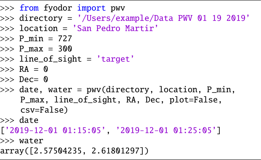
The example below displays a target with coordinates RA = 0, Dec = 0 observed from San Pedro Mártir:
Example 4. Compute PWV along the observing line of sight as observed from San Pedro Mártir.
3.5. tpw(): Compute the PWV using the TPW product
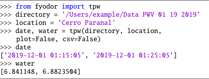
If the user prefers to use the TPW product provided by NOAA, the program can compute the PWV using the tpw function, which is a simpler version than the pwv. It needs the working directory and the locations as described for pwv. We show the working of this function using the corresponding TPW files for the same time of measurements as the examples above at Cerro Paranal:
Example 5. Compute PWV using the TPW product above Cerro Paranal.
4. Results and discussion
We analysed the amount of precipitable water vapour estimated by the program for two weeks of consecutive data from 1 December to 15 December 2019 and from 1 March to 15 March 2020. The first section contains the results of PWV above Cerro Paranal computed with the function pwv compared with data provided by LHATPRO and the TPW product. In Sect. 4.2 we present the results of the PWV above the observatory located in San Pedro Mártir. We computed the PWV between 750 hPa and 300 hPa pressure levels in Cerro Paranal and between 727 hPa and 300 hPa in San Pedro Mártir. One of the reasons we chose this upper limit is that the PWV in the TPW product is computed until that level and thus provides better conditions for comparison. The measurements were taken every 10 min by GOES-16. All times are given in UTC. The results of the PWV at zenith contain the complete number of available data excluding missing data, but the results of the PWV along the line of sight to a target in the sky in Sect. 4.3 consists of observations constrained to elevation angles above 30°. Finally, in Sect. 4.4 we briefly discuss the contribution to the PWV above the pressure level of 300 hPa. From now on, when we refer to fyodor, we mean the function pwv that is its main feature, while the results using the TPW product were retrieved using the fyodor function tpw. To clarify, when we mention fyodor measurements or results, we mean the PWV from the fyodor code using GOES data.
4.1. Comparison of the PWV above Cerro Paranal with LHATPRO data and TPW
To asses the code performance, we compared PWV data with values measured by LHATPRO, a ground-based radiometer installed at Cerro Paranal. LHATPRO measurements are publicly available for download6. We also compared the results of fyodor with the TPW product. In Fig. 2 each panel presents two weeks of measurements. In December (Fig. 2a), the difference between the highest and lowest value, called peak-to-peak value, of 2.8 mm given by fyodor is smaller than LHATPRO (5 mm) and TPW (4.6 mm), indicating that the method may be less sensitive to changes than other instruments. During the first two weeks in March (Fig. 2b), the amount of PWV is considerably higher than in December, showing a seasonal variability. The change in PWV during a single day in March is also highly variable, ranging between a difference of 1.1 mm and 4.4 mm within a day.
 |
Fig. 2. PWV above Cerro Paranal. Red points are fyodor measurements taken between 750 hPa and 300 hPa every 10 min using GOES-16 imagery data of the Full Disk region. Blue corresponds to LHATPRO, and black to the TPW product using GOES-16 imagery data from (a) 1−15 December 2019 and (b) 1−15 March 2020. |
For most of the measurements in December, the PWV given by fyodor is higher than those by LHATPRO, agreeing between each other within 3σ. In March, both datasets are similar at a significance of 0.25σ. It is clear by eye that the trend is similar. Most of the variable features are well captured by both fyodor and LHATPRO. However, some drops in PWV measured by LHATPRO, especially on 4 and 8 December 2019, are inverted in the estimation given by fyodor, resulting in an increase in PWV. For higher values, both datasets seem to agree better with each other.
From analysing all our data, it appears that the fyodor differences in values over time are less subtle than those of LHATPRO. While the general behaviour is similar between the two, LHATPRO appears to be more sensitive to PWV variations. The reason for the different values is that LHATPRO takes measurements in the range between 183 and 191 GHz (Querel & Kerber 2014), which corresponds to strong absorption lines (Matsushita & Matsuo 2002), and 51 to 58 GHz and in the range of 10 μm, while GOES-16 data are taken at different bands centred between 3.89 and 13.27 μm. The absorption coefficient of water vapour was checked in the HITRAN database (Gordon et al. 2017) for these different regions. It is highly variable and not identical for the range where LHATPRO and GOES-16 obtain measurements (see Tennyson et al. 2013; Taylor et al. 2003), which explains the absolute value difference in PWV. Another reason for the difference is that LHATPRO is an in situ instrument, guaranteeing that the measurements correspond to Cerro Paranal, while GOES-16 has a spatial resolution of 10 km, meaning that every measurement represents an average value over an area of 10 km × 10 km horizontal size. Thus, temperature and relative humidity values do not necessarily correspond to the actual values on Cerro Paranal, but to those at the nearest gridpoint on the dataset.
When we compare our results with the TPW product, both datasets also follow the same trend, capturing every drop or increase in PWV. The TPW values appear to be shifted up by an offset and stretched by a factor. The two datasets appear to be so similar, except for the shift, because the TPW end product is generated by the same algorithm that produces the legacy vertical temperature (moisture) profile and is derived from the moisture profile. However, the TPW gives an integrated value of the PWV between the surface and 300 hPa. The offset seen in the TPW product is a result of taking pressure levels into account that may not correspond to the surface pressure at a certain location. This is especially true for high-altitude locations. Running some tests with fyodor, we found that to match the offset of the TPW product, the surface pressure at Cerro Paranal should be approximately 950 hPa, while the actual mean surface pressure is approximately 750 hPa. This leads to an overestimated value of the PWV by the TPW product.
4.2. PWV above San Pedro Mártir
We computed the amount of PWV above San Pedro Mártir for the same dates using fyodor and TPW. Figures 3a and b show some notable gaps of missing data between 3 and 4 December 2019 and between 10 and 12 March 2020, probably due to partially cloudy or overcast conditions because the values of PWV before and after the gaps are relatively high. There is no evident seasonal variability between these months.
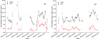 |
Fig. 3. PWV above San Pedro Mártir. Red points are fyodor measurements taken between 727 hPa and 300 hPa every 10 min using GOES-16 imagery data of the Full Disk region, and black shows the TPW product using GOES-16 imagery data from (a) 1−15 December 2019 and (b) 1−15 March 2020. |
The difference between the two measurements is analogous to the analysis above Cerro Paranal in Sect. 4.1. The trend is similar, but TPW overestimates the amount of PWV compared to fyodor. However, there are some PWV variations in the TPW product that our program does not recognise, or alternatively, the difference between the values is very small. The most drastic event occurred on 5 March 2020, where a considerable increase in PWV recorded by TPW is just a small bump in the fyodor results. Similar results are obtained on 9 and 15 March 2020, where there is even no evidence of the increase in PWV. Because TPW is a quality-checked end product, it could be that it undergoes additional processing and computation compared to the products used by fyodor.
When the PWV above San Pedro Mártir using GOES-16 imagery data is computed, the user can make use of one of the regions covering the location: Full Disk and CONUS. The Full Disk dataset has a temporal resolution of 10 min, while new data are available in the CONUS dataset every 5 min. However, during a test, we found discrepancies between the values in the datasets. The measurements are independent from each other, and usually, they do not overlap in time of measurement. However, some of the CONUS values may be extracted from the Full Disk measurement, while others are independent scans (NOAA 2019a). For a full coverage of the American region and consistency in the measurements, we recommend using the Full Disk region dataset.
4.3. PWV along the observing line of sight from Cerro Paranal and San Pedro Mártir
To prove the estimation of PWV along the line of sight, we entered a toy test target in the program with coordinates (RA) = 250 and (Dec) = −20 as seen from the observatory in Cerro Paranal. By definition, the right ascension can be related to the longitude on the great circle, while the declination corresponds to the latitude. In general, in order to compute the PWV along the line of sight, the code is ingested with two different sets of coordinates: The observing location, and the coordinates of the target in the sky. For this particular example, the test target has similar coordinates as the observatory. In this fashion, once in a 24 h cycle, it passes very close to the observatory’s zenith. The results (Figs. 4a and b) show PWV values for time intervals when the target was visible (above an elevation angle of 30°). The PWV change during an observing window in December ranges between 0.2 mm on 6 December 2019 to 1.2 mm on 4 December 2019, while in March, it ranges between 0.4 mm on 5 March 2020 to 3.1 mm on 11 March 2020. The trend is similar as above the location (see Figs. 2a and b) as well as the range of values, but there are clearly fewer data points. The reason is that by constraining to observations to above 30° altitude, the maximum projection distance is about 20 km, as discussed in Sect. 2.5, but the dataset has a resolution of 10 km. This means that the maximum change of pixels containing data points in the ABI fixed grid equals two pixels. In other words, temperature and moisture data of projection points is retrieved quite close to the observation point if not exactly at it.
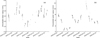 |
Fig. 4. PWV along the line of sight to a test target with coordinates RA = 250° and Dec = −20° observing from Cerro Paranal between 750 hPa and 300 hPa every 10 min using GOES-16 imagery data of the Full Disk region from (a) 1−15 December 2019 and (b) 1−15 March 2020. Data are available only when the target was visible above an elevation angle of 30°. Note the difference in the limit of the vertical axes. |
Next we computed the PWV from San Pedro Mártir along the line to a target with coordinates RA = 0°, Dec = 0°, shown in Figs. 5a and b. During a single observing window of approximately 8 h, the PWV varies as little as 0.2 mm on 2 December 2019 to 3.4 mm on 5 December 2019. In March, the smallest change during an observation is 0.3 mm on 9 March 2020, while the largest change of 1.2 mm occurs on 8 March 2020. These results reinforce the purpose for which fyodor was developed, that is, act as a supporting tool for monitoring the PWV during astronomical observations.
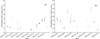 |
Fig. 5. PWV along the line of sight to a test target with coordinates RA = 0° and Dec = 0° observing from San Pedro Mártir between 727 hPa and 300 hPa every 10 min using GOES-16 imagery data of the Full Disk region from (a) 1−15 December 2019 and (b) 1−15 March 2020. Data are available only when the target was visible above an elevation angle of 30°. Note the difference in the limit of the vertical axes. |
Given that the instrumentation uncertainty in relative humidity is 18% and 1 K in temperature, our first estimates give a percentage uncertainty of about 27%. We also have to take the error into account that we induce by the numerical integration, the height approximation via barometric formula, and the formulation of the saturation vapour pressure.
4.4. Contribution to the PWV above 300 hPa
In Sect. 1 we mentioned that at heights above a pressure level of 300 hPa, the contribution to the PWV is very small, as also stated by Erasmus & van Rooyen (2006). To confirm this, we analysed our data above Cerro Paranal and San Pedro Mártir between 300 hPa and 0,005 hPa, which is the lowest pressure level available in the GOES-16 dataset.
Above Cerro Paranal the amount of PWV is still variable in time, ranging between 0.05 and 0.15 mm. Compared to the precipitable water vapour computed in Cerro Paranal between the surface and 300 hPa, the content above 300 hPa represents between 0.8% and 1.5% of it.
The results above San Pedro Mártir are similar. All values are found between 0.02 and 0.047 mm, representing 0.87% and 1.67% of the amount found between the surface and 300 hPa. Thus, we conclude that the contribution to the PWV above 300 hPa is indeed small.
5. Conclusions
The high variability of the PWV in the atmosphere is a serious challenge in the search for small exoplanets orbiting ultra-cool stars. Using GOES-16 satellite imagery data, the Python program developed here has proven to be a promising assisting tool for astronomical observation, giving an estimated value of the PWV above the site. Furthermore, we conclude that our program correctly tracks the motion of the target, benchmarking the novel method proposed here for computing the PWV along the line of sight to the target in the sky during the time of observation.
Computing the PWV using satellite-based imagery data has the advantage of being a remote-sensing method that is reasonably inexpensive for the user, allowing computations for many locations across the complete American continent. It can be very helpful at observatories within the GOES coverage that do not benefit from an on-site PWV monitoring tool. Additionally, the temporal resolution of 10 min or 5 min (depending on the dataset) allow clearly recognising temporal variability during typical observation periods in near real-time. For a single measurement, a gross estimate of the time a user would need when using fyodor to complete the process from downloading GOES data to the time when the amount of PWV is computed and saved in a .csv file is approximately 5 min for the Full Disk with a slow internet connection and approximately 30 s with a fast connection. In comparison, the whole process using the TPW product takes approximately 5 s. However, the time between requesting data from NOAA and receiving the link with the files is highly variable. The uncertainty in the PWV computed in Cerro Paranal and San Pedro Mírtir is about 27%. Compared with data in Cerro Paranal provided by LHATPRO, although the values differ, both follow a similar trend, which is favourable for the reliability of the method developed here. In general, the variability of the PWV is reasonably similar for the two methods, and the magnitudes are also similar. We recommend to compare the amount of PWV over a longer period of time to count with a statistical reliable analysis.
The TPW product provided by NOAA has the advantage of being an end product that gives the PWV value. The files are considerably smaller, and the running time of the program is also reduced. Users interested in a fast method for retrieving the amount of PWV can use this product along with the function in our program. The caveat is that it only works at the zenith on the location, and the pressure level limits are fixed between the surface and 300 hPa, which leads to an overestimated PWV value at high altitude locations. If the user needs the PWV between certain pressure levels or to follow a target during observation, they should use the pwv function of fyodor on the temperature and moisture files from GOES-16. As a supporting tool in astronomy, it is not necessary to download a complete day’s worth of data. The files corresponding to the observation time suffice.
The program was developed with the purpose of monitoring and mitigating the effect of variable PWV on astronomical observations while searching for exoplanets orbiting cool stars, but the program allows other applications to address questions on climate science or forecasting studies. The steps involved to compute PWV lead to the definition of many variables storing useful meteorologic and geographic information, which can prove helpful for modelling. From now on, the program fyodor can be used as a supporting tool during observations.
The aim of this project was to develop an open-source program that reliably computes the PWV at the request of the user. The software is intended to receive continuous maintenance and improvements. In the near future, the option to input the altitude and azimuth of a target will be implemented. Moreover, information regarding quality flags would be helpful to catalogue masked entries. NOAA provides a product containing clear sky mask and cloud mask information, which would surely improve fyodor. However, the number of files required for PWV measurements would increase. Another planned improvement is to automate the process of downloading the dataset. Right now, the user has to request the files of interest on their own at the NOAA website and then run the program to open and process them. Finally, the next great improvement is to implement a method that directly corrects for noise produced by PWV on observations. At the moment, the user can monitor the amount of PWV present during the observation at a given location, but the use given to the results is up to the user, that is, correlation or correction have to be made manually. For further research, the program will be tested with real observations.
fyodor can be downloaded at https://github.com/Erikmeier18/fyodor
Acknowledgments
We would like to thank the US National Oceanic and Atmospheric Administration (NOAA) for the Legacy Vertical Temperature Profile, Legacy Vertical Moisture Profile and Total Precipitable Water product data. We thank the anonymous referee for the constructive suggestions and comments that improved the manuscript. We are grateful to N. Schanche for her contribution to the code. B.-O. D. acknowledges support from the Swiss National Science Foundation (PP00P2-190080). This work has received support from the Centre for Space and Habitability (CSH) and the National Centre for Competence in Research PlanetS, supported by the Swiss National Science Foundation (SNSF).
References
- Ahrens, C. D. 2013, Meteorology Today: An Introduction to Weather, Climate, and the Environment (Brooks/Cole) [Google Scholar]
- Astropy Collaboration (Robitaille, T. P., et al.) 2013, A&A, 558, A33 [NASA ADS] [CrossRef] [EDP Sciences] [Google Scholar]
- Astropy Collaboration (Price-Whelan, A. M., et al.) 2018, AJ, 156, 123 [Google Scholar]
- Baker, A. D., Blake, C. H., & Sliskir, D. H. 2017, PASP, 129, 085002 [NASA ADS] [CrossRef] [Google Scholar]
- Bolton, D. 1980, Mon. Weather Rev., 108, 1046 [Google Scholar]
- Buehler, S. A., Östman, S., Melsheimer, C., et al. 2012, Atmos. Chem. Phys., 12, 10925 [Google Scholar]
- Camuffo, D. 2019, Microclimate for Cultural Heritage (Elsevier) [Google Scholar]
- Cunha, D., Santos, N. C., Figueira, P., et al. 2014, A&A, 568, A35 [NASA ADS] [CrossRef] [EDP Sciences] [Google Scholar]
- Delrez, L., Gillon, M., Queloz, D., et al. 2018, in Ground-based and Airborne Telescopes VII, eds. H. K. Marshall, & J. Spyromilio (SPIE), Int. Soc. Opt. Photon., 10700, 446 [Google Scholar]
- Demory, B. O., Pozuelos, F. J., Gómez Maqueo Chew, Y., et al. 2020, A&A, 642, A49 [CrossRef] [EDP Sciences] [Google Scholar]
- Erasmus, D., & Sarazin, M. 2002, ASP Conf. Ser., 266, 310 [Google Scholar]
- Erasmus, D. A., & van Rooyen, R. 2006, Final Report, European Southern Observatory [Google Scholar]
- Erasmus, D. A., & van Staden, C. 2001, Final Report, Cerro Tololo Inter-American Observatory [Google Scholar]
- Gillon, M., Jehin, E., Lederer, S. M., et al. 2016, Nature, 533, 221 [Google Scholar]
- Gillon, M., Triaud, A. H. M. J., Demory, B.-O., et al. 2017, Nature, 542, 456 [Google Scholar]
- Gordon, I., Rothman, L., Hill, C., et al. 2017, J. Quant. Spectrosc. Radiat. Transf., 203, 3 [Google Scholar]
- Harris, C. R., Millman, K. J., van der Walt, S. J., et al. 2020, Nature, 585, 357 [CrossRef] [PubMed] [Google Scholar]
- Hunter, J. D. 2007, Comput. Sci. Eng., 9, 90 [NASA ADS] [CrossRef] [Google Scholar]
- Jehin, E., Gillon, M., Queloz, D., et al. 2018, The Messenger, 174, 2 [NASA ADS] [Google Scholar]
- Kassomenos, P., & McGregor, G. 2006, J. Hydrometeorol., 7, 271 [Google Scholar]
- Luger, R., Sestovic, M., Kruse, E., et al. 2017, Nat. Astron., 1, 0129 [Google Scholar]
- Marín, J. C., Pozo, D., & Curé, M. 2015, A&A, 573, A41 [NASA ADS] [CrossRef] [EDP Sciences] [Google Scholar]
- Matsushita, S., & Matsuo, H. 2002, in Astronomical Site Evaluation in the Visible and Radio Range, eds. J. Vernin, Z. Benkhaldoun, & C. Muñoz-Tuñón, ASP Conf. Ser., 266, 180 [Google Scholar]
- Mile, M., Benáček, P., & Rozsa, S. 2019, Atmos. Meas. Tech., 12, 1569 [Google Scholar]
- Morris, B. M., Tollerud, E., Sipőcz, B., et al. 2018, AJ, 155, 128 [NASA ADS] [CrossRef] [Google Scholar]
- NOAA 2019a, GOES-R Series Product Definition and Users’ Guide, Volume 5 [Google Scholar]
- NOAA 2019b, GOES-R Series Product Definition and Users’ Guide, Volume 1 [Google Scholar]
- Otárola, A., Hiriart, D., & Pérez-León, J. 2009, Rev. Mex. Astron. Astrofís., 45, 161 [Google Scholar]
- Peixoto, J. P., & Oort, A. H. 1992, Physics of Climate (AIP-Press) [Google Scholar]
- Pepe, F., Cristiani, S., Rebolo, R., et al. 2021, A&A, 645, A96 [CrossRef] [EDP Sciences] [Google Scholar]
- Perrefort, D., Wood-Vasey, W. M., Bostroem, K. A., et al. 2018, PASP, 131, 025002 [Google Scholar]
- Querel, R. R., & Kerber, F. 2014, in Ground-based and Airborne Instrumentation for Astronomy V, eds. S. K. Ramsay, I. S. McLean, & H. Takami (SPIE), Int. Soc. Opt. Photon., 9147, 2941 [Google Scholar]
- Richardson, L. 2007, Beautiful Soup Documentation [Google Scholar]
- Smart, W. M. 1977, Textbook on Spherical Astronomy (Cambridge: Cambridge University Press), 25 [Google Scholar]
- Taylor, J., Newman, S., Hewison, T., & Mcgrath, A. 2003, Q. J. R. Meteorol. Soc., 129, 2949 [Google Scholar]
- Tennyson, J., Bernath, P. F., Brown, L. R., et al. 2013, J. Quant. Spectrosc. Radiat. Transf., 117, 29 [Google Scholar]
- Varmaghani, A. 2012, Terr. Atmos. Ocean. Sci., 23, 17 [Google Scholar]
- Wells, N. C. 2012, The Atmosphere and Ocean, Advancing Weather and Climate Science (Wiley-Blackwell) [Google Scholar]
Appendix A: Derivation of Eq. (5)
The specific humidity and mixing ratio w of moist air, which is the ratio of the mass of water vapour to the mass of dry air (Camuffo 2019), can be related as follows:
 (A.1)
(A.1)
Using the ideal gas equations for water vapour and dry air, considering e as the partial vapour pressure of water and pa = p − e as the partial pressure of dry air and p the atmospheric pressure, we can express the mixing ratio as
 (A.2)
(A.2)
where Ra and Rv are the gas constants for dry air and water, respectively, while Ma = 28.966 is the molecular mass of dry air, and Mv = 18.016 is the molecular mass of water. When we substitute Eq. (A.2) into Eq. (A.1), we obtain an expression for the specific humidity as a function of the pressure of water vapour and atmospheric pressure,
 (A.3)
(A.3)
The relative humidity u is defined as the ratio between the partial pressure of the vapour and its saturation vapour pressure at the same temperature and pressure. It ranges between 0 and 1 and can also be expressed in percent. We keep it as a fraction,
 (A.4)
(A.4)
Equation (A.4) is a useful way to compute the partial pressure of vapour given the relative humidity and saturation vapour pressure, which is a temperature-dependent pressure value on which a dynamic equilibrium between evaporation and condensation prevails. The functional form of the saturation pressure is given by the empirical Magnus and Tetens formula (Camuffo 2019)
 (A.5)
(A.5)
where esat(0) = 611 hPa according to Tetens’ formulation (1930), and T is given in degrees Celsius. Parameters a and b are found by empirical means. In the original formula, a = 7.5 and b = 237.3°C over a plain of water, while a = 9.5 and b = 265.5°C over a plain of ice. Although the original formula is old, it remains in use due to its simplicity and accuracy. The following equation is an improved formulation derived by Bolton (1980)
 (A.6)
(A.6)
showing lower errors than those obtained with the original formulation for temperatures below 0°C, which is the temperature range typically found over astronomical observatories located at high-altitude sites. In the range −35°C ≤ T ≤ 35°C, the maximum percentage error obtained when compared to Tetens’ formula is 1.68% at −35° C, which translates into a PWV percentage difference of approximately 0.025%. Using Eq. (A.6) in Eq. (A.4), and substituting in the expression for specific humidity (Eq. (A.3)), we can finally compute the PWV defined in Eq. (4) as a function of temperature, pressure, and relative humidity:
 (A.7)
(A.7)
The literature reports further approximations or simplifications to reduce the number of variables, for example by assuming an atmosphere of constant lapse rate, which occurs only in moisture-free atmospheres (Varmaghani 2012).
All Figures
|
Fig. 1. Illustration of where the projection points Li are located. The PWV is estimated from the observer O along the line up to the pressure level Pn. |
| In the text | |
|
Fig. 2. PWV above Cerro Paranal. Red points are fyodor measurements taken between 750 hPa and 300 hPa every 10 min using GOES-16 imagery data of the Full Disk region. Blue corresponds to LHATPRO, and black to the TPW product using GOES-16 imagery data from (a) 1−15 December 2019 and (b) 1−15 March 2020. |
| In the text | |
|
Fig. 3. PWV above San Pedro Mártir. Red points are fyodor measurements taken between 727 hPa and 300 hPa every 10 min using GOES-16 imagery data of the Full Disk region, and black shows the TPW product using GOES-16 imagery data from (a) 1−15 December 2019 and (b) 1−15 March 2020. |
| In the text | |
|
Fig. 4. PWV along the line of sight to a test target with coordinates RA = 250° and Dec = −20° observing from Cerro Paranal between 750 hPa and 300 hPa every 10 min using GOES-16 imagery data of the Full Disk region from (a) 1−15 December 2019 and (b) 1−15 March 2020. Data are available only when the target was visible above an elevation angle of 30°. Note the difference in the limit of the vertical axes. |
| In the text | |
|
Fig. 5. PWV along the line of sight to a test target with coordinates RA = 0° and Dec = 0° observing from San Pedro Mártir between 727 hPa and 300 hPa every 10 min using GOES-16 imagery data of the Full Disk region from (a) 1−15 December 2019 and (b) 1−15 March 2020. Data are available only when the target was visible above an elevation angle of 30°. Note the difference in the limit of the vertical axes. |
| In the text | |
Current usage metrics show cumulative count of Article Views (full-text article views including HTML views, PDF and ePub downloads, according to the available data) and Abstracts Views on Vision4Press platform.
Data correspond to usage on the plateform after 2015. The current usage metrics is available 48-96 hours after online publication and is updated daily on week days.
Initial download of the metrics may take a while.