| Issue |
A&A
Volume 649, May 2021
|
|
|---|---|---|
| Article Number | A179 | |
| Number of page(s) | 9 | |
| Section | The Sun and the Heliosphere | |
| DOI | https://doi.org/10.1051/0004-6361/202039381 | |
| Published online | 01 June 2021 | |
Kink instability of triangular jets in the solar atmosphere⋆
1
Institute of Physics, University of Graz, Universitätsplatz 5, 8010 Graz, Austria
e-mail: This email address is being protected from spambots. You need JavaScript enabled to view it.
2
Astronomical Institute, Slovak Academy of Sciences, 05960 Tatranská Lomnica, Slovakia
3
Leibniz-Institut für Sonnenphysik (KIS), 79104 Freiburg, Germany
4
Ilia State University, Cholokashvili Ave. 3/5, Tbilisi, Georgia
5
Abastumani Astrophysical Observatory, Mount Kanobili, Georgia
Received:
9
September
2020
Accepted:
19
February
2021
Abstract
Context. It is known that hydrodynamic triangular jets (i.e. the jet with maximal velocity at its axis, which linearly decreases at both sides) are unstable to anti-symmetric kink perturbations. The inclusion of the magnetic field may lead to the stabilisation of the jets. Jets and complex magnetic fields are ubiquitous in the solar atmosphere, which suggests the possibility of the kink instability in certain cases.
Aims. The aim of the paper is to study the kink instability of triangular jets sandwiched between magnetic tubes (or slabs) and its possible connection to observed properties of the jets in the solar atmosphere.
Methods. A dispersion equation governing the kink perturbations is obtained through matching of analytical solutions at the jet boundaries. The equation is solved analytically and numerically for different parameters of jets and surrounding plasma. The analytical solution is accompanied by a numerical simulation of fully non-linear magnetohydrodynamic (MHD) equations for a particular situation of solar type II spicules.
Results. Magnetohydrodynamic triangular jets are unstable to the dynamic kink instability depending on the Alfvén Mach number (the ratio of flow to Alfvén speeds) and the ratio of internal and external densities. When the jet has the same density as the surrounding plasma, only super-Alfvénic flows are unstable. However, denser jets are also unstable in a sub-Alfvénic regime. Jets with an angle to the ambient magnetic field have much lower thresholds of instability than field-aligned flows. Growth times of the kink instability are estimated to be 6−15 min for type I spicules and 5−60 s for type II spicules matching with their observed lifetimes. The numerical simulation of full non-linear equations shows that the transverse kink pulse locally destroys the jet in less than a minute in type II spicule conditions.
Conclusions. Dynamic kink instability may lead to the full breakdown of MHD flows and consequently to an observed disappearance of spicules.
Key words: Sun: atmosphere / Sun: oscillations / instabilities
Movies associated to Fig. 9 are available at https://www.aanda.org
© ESO 2021
1. Introduction
Flows and jets are essential building blocks of the solar atmosphere. Many different types of jets are frequently observed in the solar chromosphere and corona: spicules and mottles (Beckers 1968; De Pontieu et al. 2007; Rouppe van der Voort et al. 2009; Tsiropoula et al. 2012; Moore et al. 2011; Sterling et al. 2020), macrospicules (Pike & Mason 1998), X-ray jets (Shibata et al. 1992; Savcheva et al. 2007; Moore et al. 2013; Sterling et al. 2015, 2016, 2019), Extrem Ultraviolet (EUV) jets (Chae et al. 1999; Zhang & Ji 2014), chromospheric anemone jets (Shibata et al. 2007; Nishizuka et al. 2011), among others. Coronal X-ray jets can be driven by magnetic reconnection after the emergence of new bipolar magnetic flux (Yokoyama & Shibata 1995; Moore et al. 2011) or mini-filaments (Sterling et al. 2015, 2016; Raouafi et al. 2016), while rebound shock waves may lead to classical spicules and macrospicules (Hollweg 1982; Murawski & Zaqarashvili 2010; Murawski et al. 2011).
Hydrodynamic flows are generally unstable (Chandrasekhar 1961; Drazin & Reid 1981), which may lead to the energy dissipation and to the consecutive heating of solar atmospheric plasma. Different flow profiles lead to the different types of instabilities. The simplest is the basic flow of two fluids in parallel infinite streams of different velocities, which is subject to Kelvin-Helmholtz instability (Helmholtz 1868; Kelvin 1871). Kelvin-Helmhotz instability has been intensively observed in the solar atmosphere at boundaries of rising coronal mass ejections (Ofman & Thompson 2011; Foullon et al. 2011, 2013; Möstl et al. 2013), in solar prominences (Berger et al. 2010; Ryutova et al. 2010) and in jets (Zhelyazkov et al. 2015, 2018; Li et al. 2019). Various types of flows with smooth transverse profiles are also unstable in certain conditions (Drazin & Reid 1981). Another interesting process is connected to the transverse displacement of jet axis, which becomes unstable to the dynamic kink instability due to the centripetal force acting on flows in a curved path (Zaqarashvili 2020). The instability may lead to the observed linear transverse motions of spicule axes (De Pontieu et al. 2012; Kuridze et al. 2015) in certain conditions.
Flows with smoothed transversed profiles are more difficult to study. The simplest case is the flow with a linear transverse profile, which can be analytically studied in various situations (Drazin 2002). A jet with maximal velocity at the axis that linearly tends towards zero at boundaries is a simple model but allows relevant conclusions about jets in the solar atmosphere to be drawn. This triangular jet is unstable to the antisymmetric or kink instability for long wavelength perturbations in hydrodynamics (Drazin 2002). As the solar atmosphere is generally perceived by the magnetic field, the stability of triangular jets must be studied in magnetohydrodynamic (MHD) approximation.
A magnetic field aligned with the axis of a flow generally stabilises the sub-Alfvénic flows (Chandrasekhar 1961), while the transverse magnetic field seems to have no effect on the instabilities (Sen 1963; Ferrari et al. 1981; Cohn 1983). Therefore, the magnetic field strength (namely Alfvén Mach number, i.e. the ratio of the flow to Alfvén speeds) and topology are crucial for the threshold of flow instability. Flows with angles to the magnetic field, for example axially moving twisted magnetic flux tubes, can be always unstable (Zaqarashvili et al. 2010, 2014). The magnetic field in the solar atmosphere is highly inhomogeneous and has a complex topology. Therefore, the field may suppress the flow instability in some places, leading to the formation of relatively stable flows. However, in certain areas flows may become unstable, which leads to the heating and turbulence of plasma.
For this work, we studied the stability of triangular jets in the presence of a magnetic field in the solar atmosphere. We derived the analytical dispersion equations for antisymmetric (kink) modes of triangular jets imbedded in the external magnetic field. The dispersion equations have complex solutions in certain conditions, which indicates the instability of the jets. We also performed numerical simulations, which confirmed the analytical thresholds and growth rates. Finally, the results were applied to type I and type II spicules in the solar atmosphere, which showed an interesting coincidence of instability properties and spicule dynamics.
2. Main equations
For a stability analysis of inhomogeneous jets, we used the incompressible approximation. In general, compressibility affects the flow stability (Sen 1963), but the basic properties of the instability are still seen in the incompressible limit. Therefore, we considered single-fluid, incompressible, linearised MHD equations:
![Mathematical equation: $$ \begin{aligned} \rho \left[{{\partial }\over {\partial t}} + {\boldsymbol{V}}{\cdot }{\nabla } \right]{\boldsymbol{u}} + \rho ({\boldsymbol{u}}{\cdot }{\nabla }){\boldsymbol{V}}&=-{\nabla }p_{\rm t} + {1\over {4\pi }} ({\boldsymbol{B}}{\cdot }{\nabla }){\boldsymbol{b}}, \end{aligned} $$](/articles/aa/full_html/2021/05/aa39381-20/aa39381-20-eq1.gif) (1)
(1)
![Mathematical equation: $$ \begin{aligned} \left[{{\partial }\over {\partial t}} + {\boldsymbol{V}}{\cdot }{\nabla }\right]{\boldsymbol{b}}&= ({\boldsymbol{B}}{\cdot }{\nabla }){\boldsymbol{u}}+({\boldsymbol{b}}{\cdot }{\nabla }){\boldsymbol{V}}, \end{aligned} $$](/articles/aa/full_html/2021/05/aa39381-20/aa39381-20-eq2.gif) (2)
(2)
 (3)
(3)
where ρ, B, and V are the unperturbed density, magnetic field, and flow, while b, u, and pt are perturbations in the magnetic field, velocity, and total (hydrodynamic plus magnetic) pressure. The unperturbed magnetic field is assumed to be homogeneous. Gravity effects are neglected at this stage.
We considered a Cartesian coordinate system (x, y, z) and a plasma jet, which has a slab structure along the x axis with the half-width of d and flows in the (y, z) plane. The velocity of the jet is homogeneous with regard to y and z, but it can be either homogeneous or inhomogeneous across the slab. The unperturbed magnetic field is directed along the z axis. The solutions of Eqs. ((1)–(3)) can be searched for via normal modes: Ψ(x)expi(kyy + kzz − ωt). Then, the continuity of Lagrangian displacement and total pressure at the slab boundaries gives the dispersion relation for the normal modes with generally complex ω. We note that the incompressible limit neglects the incoming and outgoing waves from the slab (i.e. leaky modes are absent), therefore the complex frequency means real instability of the normal modes.
The magnetic field of quiet Sun regions is concentrated in thin tubes at the photospheric level. However, the tubes rapidly expand upwards in the chromosphere and may merge at some heights (Fig. 1). The plasma, which forms spicules at greater heights, may flow in three different channels: inside the tubes, between the neighbouring tubes with the same polarity, and between the tubes with opposite polarities (shown by arrows on Fig. 1). There is no firm observational evidence to confirm in which of these channels plasma flows. The different channels may support the formation of spicules with different stability properties. The direction and speed of flows strongly depend on the formation mechanism of different jets, which is beyond the scope of present paper. Here, we assumed that the jets are already formed by some mechanism, and we studied their stability for different parameters. The stability of hydromagnetic flows depends on the transverse profile of the flow and the direction of the flow with respect to the magnetic field. Before we move on to triangular jets, we briefly review the stability of homogeneous jets.
 |
Fig. 1. Possible channels of plasma flows in the solar atmosphere: (a) between neighbouring magnetic flux tubes of the same polarity; (b) inside a flux tube; (c) between neighbouring flux tubes of opposite polarities. |
3. Homogeneous jets
Homogeneous jets have been studied elsewhere, therefore we briefly describe the main properties of their instability. The main conclusion concerning stability is that the flow-aligned magnetic field stabilises the sub-Alfvénic flows (Chandrasekhar 1961; Sen 1964; Ferrari et al. 1980; Hardee & Norman 1988; Singh & Talwar 1994). However, the perpendicular magnetic field does not affect the instability, therefore one always can find the exponentially growing unstable modes in a jet that has a component perpendicular to the field.
The dispersion relation of antisymmetric perturbations for a magnetised plane jet of half-width d can be written as
![Mathematical equation: $$ \begin{aligned} \left[1+\frac{{\rho _0}}{{\rho _{\rm e}}}\tanh (kd)\right]\omega ^2&-2\frac{{\rho _0}}{{\rho _{\rm e}}}({\boldsymbol{k}}{\cdot }{\boldsymbol{V}})\tanh (kd)\omega +\frac{{\rho _0}}{{\rho _{\rm e}}}\tanh (kd)({\boldsymbol{k}}{\cdot }{\boldsymbol{V}})^2\nonumber \\&-\frac{{\rho _0}}{{\rho _{\rm e}}}\tanh (kd)({\boldsymbol{k}}{\cdot }{\boldsymbol{V}_{\rm A0}})^2-({\boldsymbol{k}}{\cdot }{\boldsymbol{V}_{\rm Ae}})^2=0, \end{aligned} $$](/articles/aa/full_html/2021/05/aa39381-20/aa39381-20-eq4.gif) (4)
(4)
where ρ0 (ρe) and VA0 (VAe) are the density and Alfvén speed inside (outside) the jet, k is the wave vector in yz-plane. This equation can be obtained from the general dispersion relation of Singh & Talwar (1994) as an incompressible limit.
If the jet is directed along the unperturbed magnetic field (i.e. V ∥ VA), where the magnetic field is assumed to have the same strength and direction inside and outside the slab for simplicity, then the phase speed is always real for any sub-Alfvénic flows (V < VA), which shows the stability of the flows. However, if the jet has an angle with the magnetic field, then the harmonics perpendicular to the magnetic field (i.e. with k ⋅ VA = 0) always have a complex phase speed, which shows the instability. Therefore, the jet, which flows at an angle to the magnetic field, is always unstable for antisymmetric perturbations. These antisymmetric perturbations cause the transverse displacement of the jet axis, similarly to kink waves in magnetic slabs (Edwin & Roberts 1982). The transverese displacements are stable in static magnetic tubes, but the flow inside the tube leads to their instability due to the centripetal acceleration (Zaqarashvili 2020).
The jet flowing inside the magnetic flux tube (the middle arrow in Fig. 1) probably follows the magnetic field. Therefore, it may not be susceptible to dynamic kink instability (Zaqarashvili 2020) and could represent the classical spicules. However, the magnetic fields can be inclined at the tube boundaries, and thus make an angle with respect to upward flows. Therefore, the flows between the tubes may have components perpendicular to the magnetic field, and hence they may be unstable due to the dynamic kink instability.
4. Triangular jets
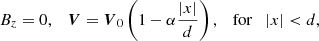
Now we consider a jet that has transverse velocity inhomogeneity, and we study how this transverse structure affects its instability properties. For simplicity, we assumed the simplest linear profile of the flow and considered a triangular jet, which has its maximum velocity at the slab axis and linearly decreases towards slab boundaries. The stability of the jet is well studied in non-magnetic fluids. It has been shown that the jet is generally unstable for long-wavelength, antisymmetric normal modes, while it is generally stable for the symmetric modes (Drazin 2002). It is in our interest to study how an external magnetic field influences the stability properties of the jet. Finding an analytical solution for MHD triangular jets is complicated, therefore we analysed the situation when a non-magnetic jet was sandwiched between two magnetic environments (Fig. 2). An especially interesting situation may arise when a jet flows between the two tubes with opposite polarities (Fig. 1c), where a neutral sheet is formed. The magnetic field becomes negligible between the tubes, and the non-magnetic jet is a good approximation.
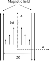 |
Fig. 2. Sketch of considered analytical setup, which corresponds to the situation of Fig. 1c. A non-magnetic triangular jet is located between the magnetic fields of opposite polarities. |
Therefore, for the triangular jet we considered
 (5)
(5)
 (6)
(6)
where the flow, V, has y and z components. The flow velocity is maximal at the slab axis and linearly decreases towards boundaries. The parameter 0 ≤ α ≤ 1 governs the rate of flow inhomogeneity. α = 0 means the homogeneous jet, which recovers the situation of previous subsection, while α = 1 describes the jet that tends towards zero at the slab boundaries. A α = 1 case was considered by Drazin (2002), but with a magnetic field free environment. In general, the flow density, ρ0, is different from the surrounding plasma, that is, ρ0 ≠ ρe (ρe is the density in external medium).
Equations ((1)–(3)) lead to the following:
![Mathematical equation: $$ \begin{aligned} \rho ({\boldsymbol{k}}{\cdot }{\boldsymbol{V}}-\omega )\left[{{\partial ^2}\over {\partial x^2}} - k^2 \right]u_x&={k_zB_z\over {4\pi }}\left[{{\partial ^2}\over {\partial x^2}} - k^2 \right]b_x, \end{aligned} $$](/articles/aa/full_html/2021/05/aa39381-20/aa39381-20-eq7.gif) (7)
(7)
 (8)
(8)
where  .
.
When ω ≠ k ⋅ V and ω ≠ kzVA, the plasma dynamics inside and outside the slab are governed by the equation
![Mathematical equation: $$ \begin{aligned} \left[{{\partial ^2}\over {\partial x^2}} - k^2 \right]u_x=0. \end{aligned} $$](/articles/aa/full_html/2021/05/aa39381-20/aa39381-20-eq10.gif) (9)
(9)
The solution to this equation is a combination of exponential functions and depends on boundary conditions on the slab centre, boundaries, and infinity.
We require the solution to vanish at infinity outside the slab, therefore the resulting expression is
 (10)
(10)
The solutions inside the slab can be antisymmetric (sinuous) or symmetric (varicose) with regard to the slab centre.
For the antisymmetric kink mode, the solution inside the jet is (Drazin 2002)
 (11)
(11)
These solutions must satisfy the continuity of Lagrangian transverse velocity and total pressure at the slab boundaries, which gives the following equations:
 (12)
(12)
![Mathematical equation: $$ \begin{aligned}&\rho \left[{\boldsymbol{k}}{\cdot }{\boldsymbol{V}}-\omega -{{k_z^2{ v}^2_{\rm A}}\over {{\boldsymbol{k}}{\cdot }{\boldsymbol{V}}-\omega }} \right]{{\partial {u_x}}\over {\partial x}}- \rho {\boldsymbol{k}}{\cdot }{\boldsymbol{V}}^{\prime }\left[1- {{k_z^2{ v}^2_{\rm A}}\over {({\boldsymbol{k}}{\cdot }{\boldsymbol{V}}-\omega )^2}}\right]u_x\nonumber \\&\qquad \qquad \qquad \qquad \qquad \quad =\mathrm{const},\quad \mathrm{at} \quad x = {\pm }d. \end{aligned} $$](/articles/aa/full_html/2021/05/aa39381-20/aa39381-20-eq14.gif) (13)
(13)
Additionally, the third equation is obtained from the pressure continuity condition at the slab centre:
![Mathematical equation: $$ \begin{aligned} \rho \left[{\boldsymbol{k}}{\cdot }{\boldsymbol{V}}-\omega \right]{{\partial {u_x}} \over {\partial x}}- \rho {\boldsymbol{k}}{\cdot }{\boldsymbol{V}}^{\prime }u_x=\mathrm{const},\quad \mathrm{at} \quad x = 0. \end{aligned} $$](/articles/aa/full_html/2021/05/aa39381-20/aa39381-20-eq15.gif) (14)
(14)
Equations (10)–(14) give the following dispersion relation for the antisymmetric mode:
![Mathematical equation: $$ \begin{aligned}&\left[1+{{\rho _0}\over {\rho _{\rm e}}}\tanh {k d}\right]\omega ^3+{\boldsymbol{k}}{\cdot }{\boldsymbol{V}_0}\left[\alpha {{\tanh {k d}}\over {k d}}-{{\rho _0}\over {\rho _{\rm e}}}(3-2\alpha )\tanh {k d}-1 \right]\omega ^2\nonumber \\&\qquad \qquad +({\boldsymbol{k}}{\cdot }{\boldsymbol{V}_0})^2\Bigg [{{\alpha ^2}\over {k d}}{{\rho _0}\over {\rho _{\rm e}}}\left(1 - {{\tanh {k d}}\over {kd}}\right)+ {{\rho _0}\over {\rho _{\rm e}}}(1-\alpha )(3-\alpha )\tanh {k d}\nonumber \\&\qquad \qquad -\frac{k_z^2V^2_{\rm A}}{({\boldsymbol{k}}{\cdot }{\boldsymbol{V}_0})^2}\Bigg ]\omega +{{\rho _0}\over {\rho _{\rm e}}}(1-\alpha )({\boldsymbol{k}}{\cdot }{\boldsymbol{V}_0})^3\Bigg [\frac{\alpha ^2}{k^2d^2}\tanh {k d} -\frac{\alpha ^2}{kd}\nonumber \\&\qquad \qquad -(1-\alpha )\tanh {k d} \Bigg ]+{\boldsymbol{k}}{\cdot }{\boldsymbol{V}_0} k_z^2V^2_{\rm A} \left[1- \alpha {{\tanh {k d}}\over {kd}}\right]=0. \end{aligned} $$](/articles/aa/full_html/2021/05/aa39381-20/aa39381-20-eq16.gif) (15)
(15)
This is a general dispersion relation, which can be analysed in different contexts.
4.1. Non-magnetised jets
If the magnetic field is negligible (VA ≈ 0), one can consider the jet in the XZ plane (i.e. ky, V0y = 0), and Eq. (15) is transformed (for α = 1) into the dispersion equation of the non-magnetised triangular jet (see Drazin 2002, Eq. (8.43)):
![Mathematical equation: $$ \begin{aligned} \left[1+{{\rho _0}\over {\rho _{\rm e}}}\tanh {k_z d}\right]\omega ^2&+k_zV_{0z}\left[{{\tanh {k_z d}}\over {k_z d}}-{{\rho _0}\over {\rho _{\rm e}}}\tanh {k_z d}-1 \right]\omega \nonumber \\&+{{k_z^2 V_{0z}^2}\over {k_z d}}{{\rho _0}\over {\rho _{\rm e}}}\left(1 - {{\tanh {k_z d}}\over {k_z d}}\right) = 0. \end{aligned} $$](/articles/aa/full_html/2021/05/aa39381-20/aa39381-20-eq17.gif) (16)
(16)
This equation has complex solutions in the interval 0 < kzd < 1.8 (i.e. the flow is unstable for long wavelength perturbations). The solution to Eq. (15) in this case is shown on Fig. 3. The frequency has an imaginary part in the interval 0 < kzd < 1.8, which vanishes for kzd > 1.8.
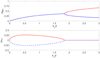 |
Fig. 3. Antisymmetric (kink) mode (Eq. (15)) solutions for the non-magnetic case (Bz = 0) when α = 1 and ky, V0y = 0 (corresponding to the solution of Drazin 2002). Upper and lower panels: real and imaginary parts of frequency, respectively. Red solid lines correspond to unstable modes, and blue dashed lines to the damped modes. Imaginary solutions (and hence instability) vanish for kzd > 1.8 and for kzd → 0. The frequency and growth rate are normalised by kzV0z. |
If the magnetic field is presented, but the flow is not parallel to the magnetic field (i.e. V0y ≠ 0), then the modes with ky ≠ 0 and kz = 0 (which are perpendicular to the magnetic field) are governed by the same equation as Eq. (16), but kz and V0z are replaced by ky and V0y. Hence, the flow is always unstable for long wavelength perturbations, even in the presence of the magnetic field. This confirms the previous results that the normal-to-flow magnetic field does not affect the Kelvin-Helmholtz instability (Chandrasekhar 1961; Sen 1964; Zaqarashvili et al. 2010, 2014).
4.2. α = 0 (homogeneous jet) limit
Next, we considered the limit of α = 0, which actually means a homogeneous jet. Then, Eq. (15) is transformed into the following equation:
![Mathematical equation: $$ \begin{aligned} \Bigg (\left[1+\frac{{\rho _0}}{{\rho _{\rm e}}}\tanh (kd)\right]\omega ^2&-2\frac{{\rho _0}}{{\rho _{\rm e}}}({\boldsymbol{k}}{\cdot }{\boldsymbol{V}_0})\tanh (kd)\omega \nonumber \\&+\frac{{\rho _0}}{{\rho _{\rm e}}}\tanh (kd)({\boldsymbol{k}}{\cdot }{\boldsymbol{V}_0})^2\nonumber \\&-k^2_z V^2_{\rm A} \Bigg )(\omega -{\boldsymbol{k}}{\cdot }{\boldsymbol{V}_0})=0. \end{aligned} $$](/articles/aa/full_html/2021/05/aa39381-20/aa39381-20-eq18.gif) (17)
(17)
When ω ≠ k ⋅ V0, then we recover Eq. (4) (with VA0 = 0). We note that Eq. (4) is transformed into the dispersion relation of Alfvén surface waves in a static magnetic slab (V0 = 0) (see Edwin & Roberts 1982, Eq. (8.43)). The antisymmetric modes are unstable when
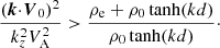 (18)
(18)
When ky = 0 and ρe = ρ0, then this inequality is replaced by 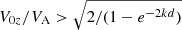 , which actually means that the flow is stabilised for all wavelength perturbations when
  . When
 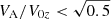 , the long wavelength perturbations are stable, while the short wavelength perturbations are unstable. The critical wave number can be estimated as
 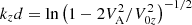 .
.
4.3. α = 1 limit
Next we consider the limit when the jet velocity vanishes at the slab boundaries (x = ±d) i.e. α = 1. In this case, Eq. (15) leads to the following equation (see also Zaqarashvili 2011):
![Mathematical equation: $$ \begin{aligned} \left[1+{{\rho _0}\over {\rho _{\rm e}}}\tanh {k d}\right]\omega ^3&+\boldsymbol{k}{\cdot }{\boldsymbol{V}_0}\left[{{\tanh {k d}}\over {k d}}-{{\rho _0}\over {\rho _{\rm e}}}\tanh {k d}-1 \right]\omega ^2\nonumber \\&+({\boldsymbol{k}}{\cdot }{\boldsymbol{V}_0})^2\left[{1\over {k d}}{{\rho _0 }\over {\rho _{\rm e}}}\left( 1 - {{\tanh {k d}}\over {kd}}\right) -\frac{k_z^2V^2_{\rm A}}{({\boldsymbol{k}}{\cdot }{\boldsymbol{V}_0})^2} \right]\omega \nonumber \\&+{\boldsymbol{k}}{\cdot }{\boldsymbol{V}_0} k_z^2V^2_{\rm A} \left[1- {{\tanh {k d}}\over {kd}}\right]=0. \end{aligned} $$](/articles/aa/full_html/2021/05/aa39381-20/aa39381-20-eq24.gif) (19)
(19)
This equation is transformed into Eq. (16) for the non-magnetised case.
Figure 4 shows the growth rates of unstable modes against a normalised wave number calculated from the dispersion relation (15) for α = 1 (solid lines) for different Alfvén Mach number values, MA = V0z/VA (the ratio of the flow speed at the slab centre and the external Alfvén speed), for ρ0/ρe = 1. It is seen that the flow is unstable only for finite intervals of the wave numbers. Therefore, only the harmonics with certain wavelengths are unstable. On the other hand, homogeneous flows (α = 0, dashed lines) are unstable when the wavelength is larger than the critical one. Sufficiently strong magnetic field suppresses the instability when  for triangular jets, which means that sub-Alfvénic flows V0z < VA are stable. However, homogeneous jets can be stabilised even for slightly super-Alfvénic regime, though they have relatively stronger growth rates.
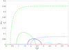 |
Fig. 4. Growth rate (imaginary part of frequency) of antisymmetric (kink) mode vs. normalised wave number kzd calculated from Eq. (15) when α = 1 and ky, V0y = 0 for different ratios of inverse Alfvén Mach number, |


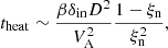
Figure 5 displays the growth rates for different Alfvén Mach number values for the denser jet, ρ0/ρe = 10. It shows that the denser jet needs stronger external Alfvén speed to stabilise the kink instability (in this case, the Alfvén speed needs to be 2.5 higher than the flow speed at the slab centre). It is clear from physical point of view that the denser jet has stronger kinetic energy and therefore it required stronger magnetic energy stabilisation.
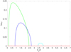 |
Fig. 5. Same as Fig. 4, but for the density ratio of ρ0/ρe = 10. Green, blue, cyan, and solid red lines correspond to |

If the flow is directed with an angle to the magnetic field (i.e. V0y ≠ 0) then the instability is not completely suppressed by the magnetic field, as was mentioned in Sect. 4.1. Figure 6 shows the growth rates of unstable modes against wave number for V0y = V0z, that is, the flow is directed at 45° to the magnetic field. In this case, the modes with the propagation angle of 45° to the magnetic field, ky/kz = 1 (dashed line), are only stabilised by a sufficiently strong magnetic field. However, the modes with a propagation angle close to 90° to the magnetic field (ky/kz = 10, solid lines) are unstable even for a very high Alfvén speed of VA/V0z = 10.
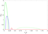 |
Fig. 6. Growth rate of antisymmetric (kink) mode vs. wave number for modes with two different propagation angles, ky/kz, when flow is directed 45° to the magnetic field, V0y/V0z = 1. The dashed green line corresponds to |


5. Discussion
Drazin (2002) showed that hydrodynamic 2D triangular jets are unstable with regard to antisymmetric kink modes, while they are stable when it comes to symmetric sausage modes. The kink modes are unstable in certain wavelength intervals, while short and long wavelength perturbations are stable (see Fig. 3). Here, we studied the influence of the magnetic field on the kink instability of triangular jets in the connection to solar atmospheric physics. In order to obtain analytical dispersion equations, we considered a triangular jet sandwiched between magnetic field tubes (or slabs), which allowed us to solve the linearised problem and led to our analytical dispersion equation (Eq. (15)) using appropriate boundary conditions.
The dispersion equation has solutions in the form of complex wave frequency, which means the instability of corresponding wave modes. The kink instability occurs at certain wave number intervals depending on the flow speed at the axis, or more precisely on the flow-to-Alfvén-speed ratio (Alfvén Mach number). Decreasing the Alfvén Mach number leads to the shortening of the instability interval and the shifting of the interval to higher wave numbers (see Fig. 4). After a certain Alfvén Mach number, the instability is terminated, hence the magnetic field stabilises the kink instability. For the density ratio of ρ0/ρe = 1, the instability ceases when  (i.e. for sub-Alfvénic flows; see Fig. 4). While for the denser jet, ρ0/ρe = 10, the instability ceases when
  (see Fig. 5). Physically, it can be understood as follows. Kink instability is related with the centripetal force, which is generated when the axis of the jet is transversally displaced so the plasma flows in a curved trajectory. This force is directed towards transverse displacement and hence tries to enhance the displacement (Zaqarashvili 2020). On the other hand, the Lorentz force tries to straighten the magnetic field lines and hence acts against the instability. A denser jet has more inertia and therefore stronger magnetic field (and consequently a lower Alfvén Mach number) is needed to stabilise the kink instability.
If the triangular jet is directed with an angle to the ambient magnetic field, then the instability may start well below the threshold (see Fig. 6). This situation may arise for inclined jets when the neighbouring magnetic field lines are vertical (as in Figs. 1a and c) or for vertical jets when the surrounding tubes are twisted. In both cases, the sub-Alfvénic jets could be unstable with regard to the dynamic kink instability. This process is related to the fact that only a flow-aligned component of the magnetic field stabilises the flow instability (Chandrasekhar 1961). The magnetic field component across the flow allows the velocity field to grow parallel to magnetic field lines without influence from the Lorentz force, hence the flow instability starts in sub-Alfvénic regimes.
The antisymmetric kink instability discussed here can be used to model the instability of various types of jets in the solar atmosphere. Here, we consider the stability of spicules as seen in obtained results. It must be mentioned, however, that the real conditions of the solar atmosphere (magnetic field structure, jet density structure, etc.) are much more complicated when compared with the simplified setup of this paper. Therefore, the results show only general properties of jet instability, which can significantly vary for different types of jets and solar atmospheric conditions.
5.1. Comparison with solar observations: instability of spicules
Spicules are chromospheric plasma jets flowing upwards into the lower corona, therefore they are almost 100 times denser and cooler than the corona. Spicules have been known for long time, as they have frequently been observed at the solar limb (Beckers 1968). A typical lifetime of the spicules is 5−15 min, and the upward velocity is ∼20−25 km s−1. We note that the disc counterparts of spicules are called mottles (Tsiropoula et al. 2012). Recent Hinode observations with high spatial and temporal resolutions revealed spicules with different properties known as type II spicules (De Pontieu et al. 2007). The type II spicules have much shorter lifetimes of 10−150 s and higher upward velocities of 50−150 km s−1 compared to classic spicules (now known as type I spicules). The disc counterparts of type II spicules are known as rapid blueshifted and rapid redshifted excursions (RBEs/RREs) and were first observed by the Swedish Solar Telescope (Rouppe van der Voort et al. 2009). The generation mechanism of spicules is poorly understood. Classical spicules can be easily formed due to rebound shocks after photospheric pulses (Hollweg 1982; Murawski & Zaqarashvili 2010), but type II spicules are more difficult to excite. Recent models of emerging bipolar regions resulting in magnetic reconnection (Moore et al. 2011; Sterling et al. 2015, 2020) or in a twist release by ambipolar diffusion (Martínez-Sykora et al. 2017) seem to capture essential features of type II spicules, though more work is required to this regard. Density and temperature are similar in both types of spicules, therefore the short lifetime of type II spicules can be caused either by their rapid diffusion or by rapid heating, which may lead to their disappearance in chromospheric spectral lines. The appearance of spicules in transition region spectral lines show that type II spicules are rapidly heated (Pereira et al. 2014), though the heating mechanism is not yet completely clear. Ion-neutral collisions, Kelvin-Helmholtz instability, or both together might lead to the rapid heating (Zaqarashvili et al. 2015; Kuridze et al. 2016; Martínez-Sykora et al. 2017; Antolin et al. 2018), but this is not yet fully established. Another possibility is that the spicules are quickly destroyed by an instability process. Zaqarashvili (2020) suggested that the dynamic kink instability of a homogeneous jet may be responsible for the disappearance of type II spicules at some height of expanding magnetic flux tubes. Here, we examine the effects of transverse flow inhomogeneity on dynamic kink instability in both types of spicules separately.
5.1.1. Kink instability in type I spicules
The diameter of type I spicules varies from 300 to 1100 km (Pasachoff et al. 2009), therefore we take a mean value of 800 km, which leads to d = 400 km for the half-width. Plasma flow may reach to 20−30 km s−1 so we take V0z = 30 km s−1 for the velocity at the jet axis (Beckers 1968; Pasachoff et al. 2009). We also assume for the external Alfvén speed in low corona as 200 km s−1 and for the density ratio of spicules and lower corona as 100. Left panels of Fig. 7 shows the solutions of the dispersion relation (15) in the parameters of type I spicules. It is seen that the jets is almost fully stabilised (red lines). Only negligible instability region around kzd = 4.5 was found. On the other hand, hydrodynamic jets are unstable in the region of kzd < 2.4, which may correspond to significantly inclined spicules. Right panels show the periods and the growth times of unstable harmonics vs. wavelength around the instability region. The period of unstable harmonics is around 23−25 s, while the growth time is 400−1000 s. The growth time of unstable harmonics is comparable to the lifetime of type I spicules, which is 5−15 min (Beckers 1968). Hence, though the instability is weak in type I spicules, it may still destroy the structure over the observed lifetime.
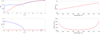 |
Fig. 7. Solutions of antisymmetric (kink) mode (Eq. (15)) in the conditions of type I spicules: ρ0/ρe = 100, d = 400 km, V0 = 30 km s−1. Left panels: real (upper) and the imaginary (lower) parts of frequencies, which are normalised by kzV0z. Blue lines show the purely hydrodynamic case (i.e. VA = 0). Red lines show the case when the external Alfvén speed is VA = 200 km s−1. Right panels: periods (upper) and growth times (lower) of unstable harmonics vs. wavelength in the interval of kzd = 4.4−4.7. Here α = 1 and ky, V0y = 0. |
5.1.2. Kink instability in type II spicules
Type II spicules are generally thinner than type I spicules with a diameter of < 200 km (De Pontieu et al. 2007), therefore we take d = 100 km for the half-width. Plasma flow may reach to 50−150 km s−1 so we take V0z = 100 km s−1 for the velocity at the jet axis. We assume the same external Alfvén speed and the density ratio as for the case of the type I spicules, that is, an Alfvén speed of 200 km s−1 and density ratio of spicules and lower corona equal to 100. The left panels of Fig. 8 show the solutions of the dispersion relation (15) in these parameters. One can see that the jets become unstable for the wave number of kzd = 0.5−2.5, which corresponds to the wavelengths of 250−1400 km. Hydrodynamic jets are again unstable in the region of kzd < 2.4. Right panels show the periods and the growth times of unstable harmonics vs. wavelength in the instability region. The period of unstable harmonics is around 5−30 s, while the growth time is 5−60 s. The growth time of unstable harmonics is comparable to the lifetime of type II spicules, which is 10−150 s (De Pontieu et al. 2007). Hence, the instability may destroy the type II spicules over the observed lifetime.
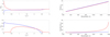 |
Fig. 8. Solutions of the antisymmetric (kink) mode (Eq. (15)) in type II spicule conditions: ρ0/ρe = 100, d = 100 km, V0 = 100 km s−1. Left panels: real (upper) and the imaginary (lower) parts of frequencies, which are normalised by kzV0z. Blue lines show the purely hydrodynamic case (i.e. VA = 0). Red lines show the case when the external Alfvén speed is VA = 200 km s−1. Right panels: periods and growth times of unstable harmonics vs. wavelength in the interval of kzd = 0.5−2.5. Here, α = 1 and ky, V0y = 0. |
5.1.3. Ion-neutral collision effects on the kink instability in spicules
Chromospheric plasma is partially ionised, therefore the collision between ions and neutral atoms may have an influence on the kink instability in spicules. Since our analysis concerns only fully ionised plasma, it is important to estimate the effects of ion-neutral collisions. Kuridze et al. (2016) estimated the heating time due to ion-neutral collision effects to be
 (20)
(20)
where  is the plasma beta, D is the spatial scale of perturbations, δin is the ion-neutral collision frequency, ξn is the neutral-to-total particle density ratio. Let us estimate the heating time for type II spicules, taking the spatial scale of unstable harmonics as D = 400 km (see previous sub-section). We take the following values for other parameters: δin = 103 Hz, β = 0.1, VA = 100 km s−1, and ξn = 0, 5 (Kuridze et al. 2016). In this case, the heating time is estimated as 3.2 × 10³ s, which is two orders of magnitude longer than the growth time of kink instability. Therefore, ion-neutral collision effects are negligible at the initial stage of instability. However, when the kink instability is fully developed, the energy is transferred to smaller scales, which in turn decreases the heating time. Therefore, an ion-neutral collision effect may only have an influence on plasma dynamics in the later stages of kink instability. This is not within the scope of the present paper and will be studied in the near future.
5.2. Numerical simulations
The analytical model considered here is obviously simplified. The solutions are linear, therefore we only model the initial linear stage of the instability, while it is also important to see the full development of the instability (i.e. what happens to the jets later on). Additionally, the absence of a magnetic field inside the jet in the considered analytical model is not a good approximation for spicules. Therefore, numerical simulations should be invoked to test the analytical results.
In this section, we present results of 2D numerical simulations obtained with the code PLUTO (e.g. Mignone et al. 2007), which accompanies our discussion in Sect. 4 on antisymmetric kink modes in a uniform background magnetic field. The code is employed to solve the ideal MHD equations in conjunction with the thermal ideal equation of state for closure. For the flux computation of an approximate Riemann solver (i.e. Harten, Lax, van Leer (HLL)) was used. A more detailed and systematic numerical analysis is underway and will be discussed in a separate paper.
Contrarily to the analytical solution (with no magnetic field inside the jet), here we consider the homogeneous magnetic field inside and outside the jet with the same strength of Bz = 10 G. For our setup, we chose typical parameters applicable to solar type II spicules. The jet’s half-width was set to d = 100 km and its speed at the axis to V0z = 100 km s−1. The inner temperature is set to 104 K. The mass density ρ0 was chosen such that a pressure equilibrium at the jet boundary is maintained, thus it depends on the external mass density of ρe = 5 × 10⁻¹⁴ g cm−3 and external temperature of Te = 4 × 10⁵ K, which means ρ0/ρe = 40. We used a cartesian grid with cell sizes of Δx = Δz = 2 km, corresponding to 1/50 of the jet’s half-width, to easily capture the turbulent evolution of the plasma flow in the non-linear regime. The initial temporal resolution was set to 5 × 10⁻⁴ s and consecutive time steps are determined by a maximum CFL number of 0.2. Neumann zero-gradient outflow boundary conditions were applied on the right as well as on the top and on bottom sides, while an open inflow condition is specified on the left boundary.
We show that the jet becomes unstable with regard to kink modes when subjected to transverse antisymmetric perturbations as discussed in Sect. 4. The perturbation amplitude of the transverse velocity was set to ∼10% of the flow speed V0z and the perturbation  of the initial Gaussian pulse
 ![Mathematical equation: $ g(z) = (\sqrt{2\pi} \sigma)^{-1} \exp\{-1/2 \cdot [(z-\upmu)/\sigma]^2\} $](/articles/aa/full_html/2021/05/aa39381-20/aa39381-20-eq37.gif) , centred around the location μ (where the initial pulse is seeded), is related to typical sizes of granulation cells. We scanned the dispersion relation, Fig. 3, for various wave numbers and indeed found a strong instability in the depicted regime. The simulation presented below is based on an initial perturbation with kzd = 1 (i.e. to the spatial scale of 628 km).
, centred around the location μ (where the initial pulse is seeded), is related to typical sizes of granulation cells. We scanned the dispersion relation, Fig. 3, for various wave numbers and indeed found a strong instability in the depicted regime. The simulation presented below is based on an initial perturbation with kzd = 1 (i.e. to the spatial scale of 628 km).
Figure 9 shows the dynamics of the plasma density, longitudinal components of velocity, and magnetic field in the jet and surroundings at different times. A significant displacement of the jet axis is already seen 15 s following the initial perturbation (second line from the top). After 45 s (bottom line), the transverse displacement already shows a non-linear character, therefore the growth time of perturbations can be estimated around 30 s, which is comparable to the analytical growth time (Fig. 8). Around 45 s after the initial perturbation, the jet is almost destroyed locally. Hence, less than 1 min after the initial excitation, the transverse velocity pulse had transformed into a fully developed local instability. If one initially excites a harmonic wave instead of local pulse, then the instability develops along the whole wave train, which collapses the jet (numerical simulations will be presented in a separate paper). This agrees with the lifetime of type II spicules fairly, therefore the spicules could be destroyed by the kink instability.
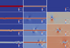 |
Fig. 9. MHD simulation of a magnetised triangular jet in type II spicule conditions. The half-width of the jet is 100 km and the total length of the simulated jet is about 7 mm. The initial transverse perturbation has an amplitude of ∼10 km s−1 (corresponding to 10% of the flow speed at the jet centre) and a spatial scale of around 600 km. We show the mass density ρ (left panels), the flow velocity Vz (middle panels), and the z-component of the magnetic field Bz (right panels) at consecutive snapshots, each 15 s apart (upper panels correspond to the initial set up). A pronounced kink develops around 30 s after initial perturbation and turns into an instability after ≈45 s. Corresponding movies can be found online. |
The propagation speed of the excited kink pulse is estimated as ≈54 km s−1 as measured in the inertial frame. The instability keeps growing until the jet is finally destroyed. The simulations show that the development of the instability critically depends on the flow speed of the jet as expected: at a lower V0z of 30 km s−1, the initially generated kink wave forms only a narrow, low amplitude pulse that is propagating with the flow without tearing down the underlying jet.
6. Conclusions
The stability of triangular jets sandwiched between two magnetic tubes (or slabs) in the solar atmosphere was studied. A dispersion equation governing the antisymmetric kink perturbations was obtained, which was solved analytically and numerically for different cases of Alfvén Mach number, MA, and the ratio of internal and external densities, ρ0/ρe. We show that triangular jets are unstable to the dynamic kink instability depending on the Alfvén Mach number and the density ratio. For example, jets with ρ0/ρe = 1 are unstable in the super-Alfvénic regime ( ), while denser jets with ρ0/ρe = 10 are unstable also in the sub-Alfvénic regime (
 ). The jets flowing with an angle to the external magnetic field become unstable well below the thresholds. The results were applied to the conditions of type I and type II spicules in the solar atmosphere. The instability growth time in the conditions of type I spicules is estimated as 6−15 min depending on the perturbation wavelength, which corresponds to the lifetime of the spicules. The instability growth time in the conditions of type II spicules is estimated as 5−60 s depending on the perturbation wavelength, which also corresponds to the lifetime of these spicules. Numerical simulations of fully non-linear MHD equations show that the initial kink pulse leads to the local breakdown of the jet in less than a minute. Consequently, the kink instability may lead to the observed short lifetime of type II spicules. However, the simple consideration of the jet and environment in this paper does not fully correspond to the real conditions in the solar atmosphere. Therefore, more work is required in the future. A more detailed numerical simulation of the process is currently underway.
Movies
Movie 1 associated with Fig. 9 (rho-movie) Access Supplementary Material
Movie 2 associated with Fig. 9 (Vz-movie) Access Supplementary Material
Movie 3 associated with Fig. 9 (Bz-movie) Access Supplementary Material
Acknowledgments
The work was funded by the Austrian Science Fund (FWF, projects P30695-N27 and I 3955-N27) and by the Deutsche Forschungsgemeinschaft (DFG, German Research Foundation) – Projektnummer 407727365. The work of TVZ and SL was funded by Georgian Shota Rustaveli National Science Foundation project DI-2016-17. SL and PG acknowledge the support of the project VEGA 2/0048/20. Acknowledgment is also given to the developers of the code PLUTO we have been using for performing the simulation presented in this paper. The authors thank the anonymous referee for stimulating comments, which led to improve the paper.
References
- Antolin, P., Schmit, D., Pereira, T. M. D., De Pontieu, B., & De Moortel, I. 2018, ApJ, 856, 44 [NASA ADS] [CrossRef] [Google Scholar]
- Beckers, J. M. 1968, Sol. Phys., 3, 367 [NASA ADS] [Google Scholar]
- Berger, T. E., Slater, G., Hurlburt, N., et al. 2010, ApJ, 716, 1288 [Google Scholar]
- Chae, J., Qiu, J., Wang, H., & Goode, P. R. 1999, ApJ, 513, L75 [NASA ADS] [CrossRef] [Google Scholar]
- Chandrasekhar, S. 1961, Hydrodynamic and Hydromagnetic Stability (Oxford: Clarendon Press) [Google Scholar]
- Cohn, H. 1983, ApJ, 269, 500 [NASA ADS] [CrossRef] [Google Scholar]
- De Pontieu, B., McIntosh, S., Hansteen, V. H., et al. 2007, PASJ, 59, S655 [Google Scholar]
- De Pontieu, B., Carlsson, M., Rouppe van der Voort, L. H. M., et al. 2012, ApJ, 752, L12 [NASA ADS] [CrossRef] [Google Scholar]
- Drazin, P. G. 2002, Introduction to Hydrodynamic Stability (Cambridge: Cambridge University Press) [Google Scholar]
- Drazin, P. G., & Reid, W. H. 1981, Hydrodynamic Stability (Cambridge: Cambridge University Press) [Google Scholar]
- Edwin, P. M., & Roberts, B. 1982, Sol. Phys., 76, 239 [NASA ADS] [CrossRef] [Google Scholar]
- Ferrari, A., Trussoni, E., & Zaninetti, L. 1980, MNRAS, 193, 469 [NASA ADS] [Google Scholar]
- Ferrari, A., Trussoni, E., & Zaninetti, L. 1981, MNRAS, 196, 1051 [NASA ADS] [Google Scholar]
- Foullon, C., Verwichte, E., Nakariakov, V. M., Nykyri, K., & Farrugia, C. J. 2011, ApJ, 729, L8 [NASA ADS] [CrossRef] [Google Scholar]
- Foullon, C., Verwichte, E., Nykyri, K., Aschwanden, M. J., & Hannah, I. G. 2013, ApJ, 767, 170 [NASA ADS] [CrossRef] [Google Scholar]
- Hardee, P. E., & Norman, M. L. 1988, ApJ, 334, 70 [NASA ADS] [CrossRef] [Google Scholar]
- Helmholtz, H. 1868, Lond. Edinb. Dublin Philos. Mag. J. Sci., 36, 337 [Google Scholar]
- Hollweg, J. V. 1982, ApJ, 257, 345 [NASA ADS] [CrossRef] [Google Scholar]
- Kelvin, W. 1871, Lond. Edinb. Dublin Philos. Mag. J. Sci., 42, 362 [Google Scholar]
- Kuridze, D., Henriques, V., Mathioudakis, M., et al. 2015, ApJ, 802, 26 [NASA ADS] [CrossRef] [Google Scholar]
- Kuridze, D., Zaqarashvili, T. V., Henriques, V., et al. 2016, ApJ, 830, 133 [NASA ADS] [CrossRef] [Google Scholar]
- Li, X., Zhang, J., Yang, S., & Hou, Y. 2019, ApJ, 875, 52 [CrossRef] [Google Scholar]
- Martínez-Sykora, J., De Pontieu, B., Hansteen, V. H., et al. 2017, Science, 356, 1269 [NASA ADS] [CrossRef] [Google Scholar]
- Mignone, A., Bodo, G., Massaglia, S., et al. 2007, ApJS, 170, 228 [Google Scholar]
- Moore, R. L., Sterling, A. C., Cirtain, J. W., & Falconer, D. A. 2011, ApJ, 731, L18 [NASA ADS] [CrossRef] [Google Scholar]
- Moore, R. L., Sterling, A. C., Falconer, D. A., & Robe, D. 2013, ApJ, 769, 134 [NASA ADS] [CrossRef] [Google Scholar]
- Möstl, U. V., Temmer, M., & Veronig, A. M. 2013, ApJ, 766, L12 [NASA ADS] [CrossRef] [Google Scholar]
- Murawski, K., & Zaqarashvili, T. V. 2010, A&A, 519, A8 [NASA ADS] [CrossRef] [EDP Sciences] [Google Scholar]
- Murawski, K., Srivastava, A. K., & Zaqarashvili, T. V. 2011, A&A, 535, A58 [NASA ADS] [CrossRef] [EDP Sciences] [Google Scholar]
- Nishizuka, N., Nakamura, T., Kawate, T., Singh, K. A. P., & Shibata, K. 2011, ApJ, 731, 43 [NASA ADS] [CrossRef] [Google Scholar]
- Ofman, L., & Thompson, B. J. 2011, ApJ, 734, L11 [NASA ADS] [CrossRef] [Google Scholar]
- Pasachoff, J. M., Jacobson, W. A., & Sterling, A. C. 2009, Sol. Phys., 260, 59 [NASA ADS] [CrossRef] [Google Scholar]
- Pereira, T. M. D., De Pontieu, B., Carlsson, M., et al. 2014, ApJ, 792, L15 [NASA ADS] [CrossRef] [Google Scholar]
- Pike, C. D., & Mason, H. E. 1998, Sol. Phys., 182, 333 [NASA ADS] [CrossRef] [Google Scholar]
- Raouafi, N. E., Patsourakos, S., Pariat, E., et al. 2016, Space Sci. Rev., 201, 1 [Google Scholar]
- Rouppe van der Voort, L., Leenaarts, J., de Pontieu, B., Carlsson, M., & Vissers, G. 2009, ApJ, 705, 272 [NASA ADS] [CrossRef] [Google Scholar]
- Ryutova, M., Berger, T., Frank, Z., Tarbell, T., & Title, A. 2010, Sol. Phys., 267, 75 [Google Scholar]
- Savcheva, A., Cirtain, J., Deluca, E. E., et al. 2007, PASJ, 59, S771 [NASA ADS] [CrossRef] [Google Scholar]
- Sen, A. K. 1963, Phys. Fluids, 6, 1154 [NASA ADS] [CrossRef] [Google Scholar]
- Sen, A. K. 1964, Phys. Fluids, 7, 1293 [Google Scholar]
- Shibata, K., Ishido, Y., Acton, L. W., et al. 1992, PASJ, 44, L173 [NASA ADS] [CrossRef] [Google Scholar]
- Shibata, K., Nakamura, T., Matsumoto, T., et al. 2007, Science, 318, 1591 [NASA ADS] [CrossRef] [Google Scholar]
- Singh, A. P., & Talwar, S. P. 1994, Sol. Phys., 149, 331 [NASA ADS] [CrossRef] [Google Scholar]
- Sterling, A. C., Moore, R. L., Falconer, D. A., & Adams, M. 2015, Nature, 523, 437 [Google Scholar]
- Sterling, A. C., Moore, R. L., Falconer, D. A., et al. 2016, ApJ, 821, 100 [Google Scholar]
- Sterling, A. C., Harra, L. K., Moore, R. L., & Falconer, D. A. 2019, ApJ, 871, 220 [Google Scholar]
- Sterling, A. C., Moore, R. L., Samanta, T., & Yurchyshyn, V. 2020, ApJ, 893, L45 [Google Scholar]
- Tsiropoula, G., Tziotziou, K., Kontogiannis, I., et al. 2012, Space Sci. Rev., 169, 181 [NASA ADS] [CrossRef] [Google Scholar]
- Yokoyama, T., & Shibata, K. 1995, Nature, 375, 42 [NASA ADS] [CrossRef] [Google Scholar]
- Zaqarashvili, T. V. 2011, in American Institute of Physics Conference Series, eds. I. Zhelyazkov, & T. Mishonov, 1356, 106 [Google Scholar]
- Zaqarashvili, T. V. 2020, ApJ, 893, L46 [Google Scholar]
- Zaqarashvili, T. V., Díaz, A. J., Oliver, R., & Ballester, J. L. 2010, A&A, 516, A84 [NASA ADS] [CrossRef] [EDP Sciences] [Google Scholar]
- Zaqarashvili, T. V., Vörös, Z., & Zhelyazkov, I. 2014, A&A, 561, A62 [NASA ADS] [CrossRef] [EDP Sciences] [Google Scholar]
- Zaqarashvili, T. V., Zhelyazkov, I., & Ofman, L. 2015, ApJ, 813, 123 [NASA ADS] [CrossRef] [Google Scholar]
- Zhang, Q. M., & Ji, H. S. 2014, A&A, 561, A134 [NASA ADS] [CrossRef] [EDP Sciences] [Google Scholar]
- Zhelyazkov, I., Zaqarashvili, T. V., Chandra, R., Srivastava, A. K., & Mishonov, T. 2015, Adv. Space Res., 56, 2727 [Google Scholar]
- Zhelyazkov, I., Zaqarashvili, T. V., Ofman, L., & Chandra, R. 2018, Adv. Space Res., 61, 628 [Google Scholar]
All Figures
|
Fig. 1. Possible channels of plasma flows in the solar atmosphere: (a) between neighbouring magnetic flux tubes of the same polarity; (b) inside a flux tube; (c) between neighbouring flux tubes of opposite polarities. |
| In the text | |
|
Fig. 2. Sketch of considered analytical setup, which corresponds to the situation of Fig. 1c. A non-magnetic triangular jet is located between the magnetic fields of opposite polarities. |
| In the text | |
|
Fig. 3. Antisymmetric (kink) mode (Eq. (15)) solutions for the non-magnetic case (Bz = 0) when α = 1 and ky, V0y = 0 (corresponding to the solution of Drazin 2002). Upper and lower panels: real and imaginary parts of frequency, respectively. Red solid lines correspond to unstable modes, and blue dashed lines to the damped modes. Imaginary solutions (and hence instability) vanish for kzd > 1.8 and for kzd → 0. The frequency and growth rate are normalised by kzV0z. |
| In the text | |
|
Fig. 4. Growth rate (imaginary part of frequency) of antisymmetric (kink) mode vs. normalised wave number kzd calculated from Eq. (15) when α = 1 and ky, V0y = 0 for different ratios of inverse Alfvén Mach number, |
| In the text | |
|
Fig. 5. Same as Fig. 4, but for the density ratio of ρ0/ρe = 10. Green, blue, cyan, and solid red lines correspond to |
| In the text | |
|
Fig. 6. Growth rate of antisymmetric (kink) mode vs. wave number for modes with two different propagation angles, ky/kz, when flow is directed 45° to the magnetic field, V0y/V0z = 1. The dashed green line corresponds to |
| In the text | |
|
Fig. 7. Solutions of antisymmetric (kink) mode (Eq. (15)) in the conditions of type I spicules: ρ0/ρe = 100, d = 400 km, V0 = 30 km s−1. Left panels: real (upper) and the imaginary (lower) parts of frequencies, which are normalised by kzV0z. Blue lines show the purely hydrodynamic case (i.e. VA = 0). Red lines show the case when the external Alfvén speed is VA = 200 km s−1. Right panels: periods (upper) and growth times (lower) of unstable harmonics vs. wavelength in the interval of kzd = 4.4−4.7. Here α = 1 and ky, V0y = 0. |
| In the text | |
|
Fig. 8. Solutions of the antisymmetric (kink) mode (Eq. (15)) in type II spicule conditions: ρ0/ρe = 100, d = 100 km, V0 = 100 km s−1. Left panels: real (upper) and the imaginary (lower) parts of frequencies, which are normalised by kzV0z. Blue lines show the purely hydrodynamic case (i.e. VA = 0). Red lines show the case when the external Alfvén speed is VA = 200 km s−1. Right panels: periods and growth times of unstable harmonics vs. wavelength in the interval of kzd = 0.5−2.5. Here, α = 1 and ky, V0y = 0. |
| In the text | |
|
Fig. 9. MHD simulation of a magnetised triangular jet in type II spicule conditions. The half-width of the jet is 100 km and the total length of the simulated jet is about 7 mm. The initial transverse perturbation has an amplitude of ∼10 km s−1 (corresponding to 10% of the flow speed at the jet centre) and a spatial scale of around 600 km. We show the mass density ρ (left panels), the flow velocity Vz (middle panels), and the z-component of the magnetic field Bz (right panels) at consecutive snapshots, each 15 s apart (upper panels correspond to the initial set up). A pronounced kink develops around 30 s after initial perturbation and turns into an instability after ≈45 s. Corresponding movies can be found online. |
| In the text | |
Current usage metrics show cumulative count of Article Views (full-text article views including HTML views, PDF and ePub downloads, according to the available data) and Abstracts Views on Vision4Press platform.
Data correspond to usage on the plateform after 2015. The current usage metrics is available 48-96 hours after online publication and is updated daily on week days.
Initial download of the metrics may take a while.