| Issue |
A&A
Volume 649, May 2021
|
|
|---|---|---|
| Article Number | A57 | |
| Number of page(s) | 7 | |
| Section | Stellar structure and evolution | |
| DOI | https://doi.org/10.1051/0004-6361/201936784 | |
| Published online | 11 May 2021 | |
Chirp mass–distance distributions of the sources of gravitational waves
Institute of Theoretical Physics, Faculty of Physics, University of Warsaw, Pasteura 5, 02-093 Warsaw, Poland
e-mail: This email address is being protected from spambots. You need JavaScript enabled to view it.
Received:
25
September
2019
Accepted:
26
January
2021
Abstract
Context. The detection of gravitational waves emitted by binary black holes raises questions regarding the origin of binaries. There are several models in the literature involving binary evolution in both the field and clusters.
Aims. We compare the predictions of these models with observations and establish the reliability of this comparison.
Methods. We use the likelihood calculation to compare the models in the space spanned by the observed chirp mass and the luminosity distance of the source.
Results. We rank the models by their ability to explain all current gravitational wave detections. It is shown that the most probable models correspond to binary evolution with low metallicity. Several variants of such evolution have similar likelihoods. The globular cluster model, considered here, is disfavoured.
Conclusions. We present the usefulness of the method in distinguishing between models when new observations become available. We calculate the number of observations required to distinguish between each pair of models. We find that the number varies from ten to several thousand for some pairs of models, yet almost two-thirds of pairs are distinguishable with at most 100 observations.
Key words: gravitational waves / stars: black holes
© ESO 2021
1. Introduction
The discovery of gravitational waves (GWs; Abbott et al. 2016) marked the beginning of gravitational wave astronomy. The recent catalogue of gravitational wave sources (The LIGO Scientific Collaboration & the Virgo Collaboration 2019; Abbott et al. 2020) contains 50 candidates, 47 of which are binary black hole (BBH) mergers. The properties of the population were studied by Belczynski et al. (2017). In the mean time, several models of formation of BBHs have been proposed. The leading model is based on the assumption that all these sources form as a result of binary evolution. This idea has been explored by several authors in recent decades (Lipunov et al. 1997; Belczynski et al. 2002, 2008; Dominik et al. 2012). Recently a version of this scenario in which the stars undergo strong mixing and have uniform chemical composition was studied as an alternative option. Additionally, several authors discuss the possibility of enhanced formation of BBHs in globular clusters (Rodriguez et al. 2016; Askar et al. 2017).
The availability of data for 47 BBH mergers allows the model predictions to be compared with observations. We present these comparisons using Bayesian statistical inference. The paper is organised as follows: In Sect. 2 we present the principles of detection of BBHs, and Sect. 3 contains a description of the statistical method used. In Sect. 4 we present the models of BBH populations used for comparison and in Sect. 5 we discuss the properties of the populations that are important for this analysis. In Sect. 6 we briefly explain why signal-to-noise ratio distributions carry little information about the population that is useful for the Advanced Laser Interferometer Gravitational-Wave Observatory (LIGO), and finally in Sect. 7 we present results of the analysis of the chirp mass–luminosity distance distributions in the context of current detections and the possibility of distinguishing between models when more data become available.
2. Detection in binary systems
Consider a BBH with masses m1 and m2, which is moving in a circular orbit. Peters & Mathews (1963) showed that those systems will emit energy via GWs. The waveform of these GWs depends on the redshifted chirp mass ℳz = ℳ(1 + z), where chirp mass is defined as
The position of the BBH on the sky with respect to the detector is described in spherical coordinates by angles θ and ϕ. The orientation of the BBH is described by the angles ι and ψ in spherical coordinates, where the z-axis is parallel to the total angular momentum of the system (Finn 1996). Measuring distance to the system must take the geometry of spacetime into account. These cosmological effects are encompassed by the luminosity distance
where  and DH = c/H0. We use the following parameters: Ωm = 0.27, ΩΛ = 1 − Ωm = 0.73, and H0 = 70.4 km s−1 Mpc−1. We assume that the BBH will be detected if its signal-to-noise ratio (S/N) ρ is greater than 8. The S/N here is defined as
 (1)
(1)
where A(ℳz) is the luminosity distance at which an optimally oriented binary with redshifted chirp mass ℳz is detected with an S/N of four and Θ(θ, ϕ, ι, ψ) is the sensitivity of the detector to the orientation of the BBH. The orientation sensitivity Θ ∈ [0, 4] is
![Mathematical equation: $$ \begin{aligned} \Theta (\theta , \phi , \iota , \psi )= 2[F^2_+(1+\cos ^2\iota )^2+4F^2_\times \cos ^2 \iota ]^{1/2}, \end{aligned} $$](/articles/aa/full_html/2021/05/aa36784-19/aa36784-19-eq5.gif)
where F+ and F× are the sensitivity of the detector to polarisations + and × of the GW (Finn 1996) defined as
 (2)
(2)
 (3)
(3)
We consider the Advanced LIGO in configuration H1 (Martynov et al. 2016). The purpose of this choice is twofold: (i) to determine which model is preferred by up-to-date observations and (ii) to determine if this detector configuration is capable of differentiating between models. For ℳz ≤ 100 M⊙, the dependence of the sensitivity of Advanced LIGO on chirp mass can be approximated by  , which leads to the commonly used approximation of S/N
  . The full range of A(ℳz), which is twice the horizon luminosity distance (i.e. distance for which ρ = 8 for a given detector), is presented in Fig. 1.
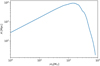 |
Fig. 1. Response of Advanced LIGO to the observed chirp mass. |
The dependence of sensitivity on chirp mass essentially encapsulates the ability of the interferometer to detect different frequencies which is a function of detector construction and corresponding noises. The main sources of the noise are seismic noises directly moving interferometer mirrors, thermal noise interacting with the beam, and quantum noise producing fluctuations in the number of photons in the beam. A full discussion on the noise sources can be found in Martynov et al. (2016).
3. Method of distinguishing models
To distinguish between the models we employ the method of statistical Bayesian inference. A broader description of this approach can be found in Gregory (2005). For the purpose of this analysis let us define:
-
P(Mi|∣)
probability that model Mi is correct, given observation O
-
P(∣|Mi)
]] probability of observing O, given that modelMi is correct
-
P(Mi)
]] prior probability that model Mi is correct.
We note that
 (4)
(4)
where ℒ(O ∣ Mi) is the likelihood function for the model Mi, ℬ is the set of investigated observables, and k indexes the observations in 𝒪. Furthermore, we denote O as Oi to emphasise that is was generated using model Mi. The probability distribution of ℬ = (DL, ℳ) for a given model is defined as follows:
 (5)
(5)
where for a given model Mi we estimate the above probability by calculating a set of 105 observations labelled by l and characterised by (DLl, ℳl). The delta function is approximated using the value of the nearest bin on a 200 by 200 grid. Subsequently, for a model Mi we can calculate the likelihood of this model given up-to-date, real GW observations by
 (6)
(6)
where n covers the set of the real GW observations. Assuming that we are in the position of maximal ignorance with regard to the validity of the model, we let all P(Mi) be equal. Then, following Gregory (2005), let us define the Bayes factor as
 (7)
(7)
where the second equality is a result of the Bayes theorem,
where P(Oi) is the normalisation.
We would like to point out that Fij ≫ 1 means that observation Oi is in favour of model Mi over Mj and thus suggests that the former better represents reality than the latter. We analyse distributions of Bayes factors for different models to establish the threshold of distinguishability with p-value α. The threshold of distinguishability (TOD) with p-value α is defined as the minimal number of observations needed for (1 − α)×100% of the Bayes factors Fij to be greater than 1. To avoid numerical noise we also require that the same inequality holds for every number of the observations greater than the threshold. The process of calculating the TOD is as follows:
1. Generate an observation Oi using model Mi.
2. For each pair of models, calculate Fij using the number of observations ranging logarithmically from 3 to 3000.
3. Repeat the previous point 104 times if the number of observations in Oi is smaller than 10 or 103 times otherwise, then analyse the distributions of the Bayes Factor based on this sample.
We note the following characteristics of this approach:
– There is no symmetry in reversing the models  . This is because those Bayes factors use observations based on different models.
– The mean value of Fij is expected to be greater than 1. Similarly to the previous point, this is is because on average obtaining Oi is more probable with Mi than with Mj. This stresses the importance of using a high enough p-value.
– The TOD is dependent on the choice of the detector and the set of observables ℬ.
4. Investigated models
We surveyed a total of 34 models for compatibility with up-to-date observations. Additionally, 16 out of the above 34 models were surveyed for distinguishability based on their ability to explain observations. Of those 34 models, 32 are StarTrack models available online1. To minimise numerical error it was additionally required that a model have at least 100 systems evolved to BBH. We now present an abridged description of the models; for the full description of the StarTrack models we refer to Dominik et al. (2012). The two non-StarTrack models are chemically homogeneous evolution and evolution in globular clusters.
4.1. StarTrack models
StarTrack is a population synthesis code focused on evolution of field stars and binary systems (Belczynski et al. 2002, 2008). It incorporates a twofold treatment of the Hertzsprung Gap donors in a common envelope (CE) phase. In the family of models B, the CE phase initiated by a Hertzsprung Gap donor always leads to a merger and formation of a Throne-Żytkow object. These models usually do not form a sufficient number of BBHs to explain observations.
In the family of models A, the energy balance is calculated following the Webbink (1984) formalism as
 (8)
(8)
where i and f stand for the initial and final, and Mdon, Macc, and Mdon, env are the masses of the donor, the accretor, and the ejected envelope. Rdon, lob is the Roche lobe radius of the donor at the beginning of the Roche Lobe Overflow (ROFL) and A is the binary separation. The energy balance determines whether the binary will shed its envelope, merge during CE, or coalesce. The λ parameter is used in energy balance of CE and is defined as
 (9)
(9)
where Ebind is the binding energy of the envelope and R is the radius of the donor.
The compact object merger can only occur if the binary survives the CE phase or phases. Therefore, we consider only the family of models A. StarTrack models can be categorised according to differences in the input physics: CE energy parameter λ, maximum neutron star (NS) mass, natal kick velocity, supernova engine, wind loss, and mass transfer treatment; for a more detailed discussion see Dominik et al. (2012). We used the model files published at the website syntheticuniverse.org and the description below refers to the models provided on that site.
4.1.1. Standard model
Standard model uses the λ parameter varying during evolution according to Xu & Li (2010), which is dubbed as Nanjingλ. Maximal NS mass is taken to be 2.5 M⊙. The mass transfer is half-conservative (half of the mass is ejected to infinity). This means that fa = 0.5, defined as Ṁacc = faṀdon, where Ṁacc is ROFL mass transfer rate and Ṁdon is the ROFL mass transfer rate of the donor. Natal kick distribution is Maxwellian with σ = 265 km s−1 and the fall-back factor ffb is according to Fryer et al. (2012). The fall-back factor ffb is defined as vk = vmax(1 − ffb), where vmax is velocity drawn from the Maxwellian distribution and vk is the final velocity. The Standard model uses a Rapid supernova engine, as described in Fryer et al. (2012).
4.1.2. Variants
In Table 1 we present variants of the StarTrack model. Parameters other than those mentioned under ‘Changed parameter’ remain the same as in the Standard model.
Variants of StarTrack model.
4.2. Other models
1. Chemically homogeneous evolution (CHE): One of the alternative channels of BBH evolution is CHE, described in de Mink & Mandel (2016). Here we study the model denoted ‘Default’ in Mandel & de Mink (2016). Owing to rapid rotation causing transport of matter between the core and the surface, CHE systems do not have a chemical gradient. Such stars gradually shrink, staying inside the Roche Lobe, and omit a transfer phase. Because of their non-violent evolution, the resulting BBHs may have a higher mass than is typical for these objects.
2. Globular Clusters (GCs): Morscher et al. (2013) suggest that the merger rate in GCs may be comparable to the rate in the field evolution. Because of this we include a GC model simulated with MOCCA code (Giersz et al. 2013) and broadly described in Askar et al. (2017). This model is a sum of approximately 2000 submodels with varying initial conditions: Z ∈ [0.002 − 0.02] and distance from the galaxy centre between 1 and 50 kpc. All submodels share the Maxwellian natal velocity kick distribution with σ = 265 km s−1, the rotational velocity of a cluster of 220 km s−1, and the IMF according to Kroupa (2001). The simulated GCs agree with observations of GCs in the Galaxy (Askar et al. 2017). Coalescing in a GC leads to faster BBH evolution, while those expelled and coalescing outside are subject to slower evolution; both scenarios are considered.
5. Characteristics of BBH population
We consider a space of three (not entirely independent) observables: {ρ, ℳ, DL}. We also show in Sect. 6 that the luminosity distributions contain little information, and therefore we limit our analysis to two-dimensional chirp mass–luminosity distance distributions. For the purpose of this analysis, the BBH models have only two characteristic attributes: intrinsic chirp mass distribution and spatial distribution.
We have (Taylor et al. 2012)
 (10)
(10)
where ṅ(z) is the merger rate density containing information about the rate of merging of the BBH at a given redshift and 𝒫(ℳ) is the observed chirp mass distribution (in contrast to the intrinsic chirp mass distribution used by Taylor et al. 2012). If  is comoving distance and Vc is comoving volume, then
Integrating Eq. (10) over Θ, neglecting the time dependence, and substituting the variable z for DL we get
 (11)
(11)
which we use as P(O ∣ Mi), setting ℬ to be {DL, ℳ}.
Alternatively, integrating over ℳ and Θ we get
 (12)
(12)
which is, when normalised, the probability of observing an event originating in the coalescence at the redshift z (regardless of its S/N). To choose the normalisation we limit redshift to zmax, which is the solution of equation  for the greatest mass in the model. Figure 2 presents the distributions of merger rate density. Because ṅ enters Eq. (12) linearly, and this equation itself is normalised, the absolute magnitude of merger rate density is unimportant.
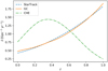 |
Fig. 2. Normalised merger rate distributions of the used models. The dashed, solid, and dot-dashed lines correspond to StarTrack, GC, and CHE models, respectively. StarTrack merger rate density is taken from model M10 from Belczynski et al. (2017). |
In Fig. 3 we present the chirp mass distributions of CHE and GC models. The distributions for the StarTrack models can be found in Dominik et al. (2012); they typically average around 7 M⊙ for Z = 1 Z⊙ and under 14 M⊙ for Z = 0.1 Z⊙.
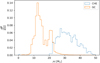 |
Fig. 3. Normalised intrinsic chirp mass distributions. The solid line corresponds to the GC model and the dashed line corresponds to the CHE model. |
6. Luminosity distribution
Before investigating the mass–distance distribution, let us first consider a luminosity distribution. Because of the short range of Advanced LIGO (compared to other third-generation detectors, e.g., the Einstein Telescope) we can approximate the luminosity distance DL with a physical distance R. In Eq. (1), we have R ∝ ρ−1. Then, assuming a uniform distribution of sources and a single value of mass, we have N ∝ V ∝ R3 ∝ ρ−3 and  . This raises a concern that, unless the BBH spatial distributions are sufficiently different, all S/N distributions may show little deviation from ρ−4.
We demonstrate in Fig. 4 that for the majority of the events the distributions follow the theoretical curve, with only the most luminous events showing a difference. For this reason, we investigated the distributions of chirp mass–luminosity distance instead of S/N. The difference between the theoretical curve and calculations in the case of the most luminous events with ρ > 102 is mostly due to the mass distribution of merging BBHs. The heavy BBHs contribute to the tail with high ρ if the events are nearby, while for smaller values of ρ the S/N distribution is averaged over the large volume where events are detectable.
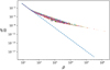 |
Fig. 4. Normalised S/N distribution. The dashed line represents the theoretical curve, with ρmin = 8. Other curves are the distributions of 16 simulated models (listed in Sect. 7.1) based on 105 binaries. |
7. Results
7.1. Likelihoods
The updated list of GW observations can be found in the catalogues by The LIGO Scientific Collaboration & the Virgo Collaboration (2019) and Abbott et al. (2020) These observations are used in the calculation of the likelihood of explaining the observations by any single model (6). The likelihoods are calculated according to Eq. (4) with the chirp mass–luminosity distance taken as P(D ∣ Mi). In the calculation of probabilities, the errors are accounted for by weighting the probabilities with Gaussian distributions corresponding to the measurement uncertainty of the given observations.
Selected models with the highest likelihood are subsequently examined for distinguishability using Bayesian inference in Sect. 7.2. We present those likelihoods in Fig. 5. The demarcation point is the natural one; the likelihood of the next most likely model when compared to the likelihood of the Standard model is of the order of the numerical error.
 |
Fig. 5. Likelihoods for the 16 selected models that could explain all of the selected GW observations. The likelihoods are normalised by the likelihood of the Standard StarTrack model. |
All of the solar metallicity StarTrack models could explain only the closest observations with the smallest mass, with chirp mass of several solar masses and distance of less then 800 Mpc. On the contrary, the chirp mass distribution of the CHE model is too high to explain the mergers with chirp mass lower than 20 M⊙. The StarTrack models with Z = 0.1 Z⊙ (with exception of the Variant 4 whose intrinsic mass distribution is too small) and GC are selected for calculations of thresholds. It is worth emphasising that none of the models are capable of explaining observations further than 3 Gpc.
Variant 9, characterised by no BH natal kick, is the most probable model with likelihood ≈3.5 times higher than the Standard model. Several models are slightly preferred to the Standard model: V5, V6, V7, and V9. Those models differ from the Standard model in that they have either a higher or lower NS mass and lower or no natal kick, respectively. Still none of these likelihoods are sufficiently high for the model to be a meaningful alternative to the Standard model. Any change to λ decreases the likelihood of the model by a factor of at least 100. An increase in wind mass loss (V11) reduces the likelihood by 8 orders of magnitude. Finally, the observations strongly disfavour the GC model, as it is less likely by 15 orders of magnitude.
7.2. Thresholds of distinguishability
For the calculation of the TOD, the data Oi are taken to have Gaussian errors with
which are average relative errors for all real observations. It should be noted that because the catalogues give a 90% symmetric interval error, the above errors were scaled to correspond to a standard deviation. Although the errors cited by the catalogues are not Gaussian, they differ from Gaussian mainly at the tails of the distribution and thus approximation is appropriate. The purpose of calculating the thresholds is to check whether likelihoods in the Fig. 5 are reliable with probability α, given the available number of observations. Table 2 suggests that two groups of parameters can be distinguished (i.e. thresholds for all pairs are under 47) with the current number of observations: wind mass reduction (Standard, V11) and λ = const (V1, V2, V3, also for the purpose of the comparison Standard). Comparing this result with Fig. 5 we can conclude that changes to the Standard model parameters are unpreferable. Some groups of parameters are distinguishable, except for distinguishing with the Standard model. In this group there are: BH natal kick (V8, V9), mass transfer (V12, V13), and Nanjing λ (V14, V15). If for other reasons the Standard model would not be preferable, the results for those groups point to the likely correction of the parameters. The remaining groups: maximal NS mass (V5, V6), natal kick distribution (V7), and SN engine (V10) are not distinguishable. Finally, the GC, V11, and V13 models are (separately) distinguishable from the rest of the models. The overall situation may change if research based on other evidence limits the available model space.
Thresholds of distinguishability with p-value α = 0.1.
Thresholds of distinguishability with p-value α = 0.01.
An unexpected result is the strong anti-symmetry of the TOD for some models. We do not expect full symmetry in Tables 2 and 3 because the corresponding TODs are calculated using different observations. Still, in some cases, breaking of this symmetry is extreme enough that we propose an explanation based on the distributions for Standard StarTrack model and Variant 12 with metallicity Z = 0.1 Z⊙. If we assume that Variant 12 is correct, we can exclude the Standard model with only 28 observations (p-value = 0.9); yet the reverse is not true even for 3000 observations. The probability distribution of both models is concentrated in the area around ℳ ≈ 28 M⊙. For Variant 12 the probability distribution is denser in this area than for the Standard model, while the latter distribution is overall more uniform. This fact is understated in Figs. 6 and 7 due to the logarithmic scale. When generating observations using Variant 12 one quickly exceeds the expected density for the Standard model, therefore the Variant 12 is distinguishable from the Standard model. On the other hand, more observations must be generated using the more uniform distribution of the Standard model in order to see that the density in the ℳ ≈ 28 M⊙ area is not as high as expected for Variant 12.
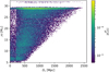 |
Fig. 6. Chirp mass–luminosity distance distribution for the Standard StarTrack model with Z = 0.1 Z⊙. |
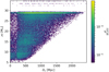 |
Fig. 7. Chirp mass–luminosity distance distribution for Variant 12 of the StarTrack model with Z = 0.1 Z⊙. |
8. Conclusions
Tables 2 and 3 show that given 100 observations we will likely be able to distinguish between almost 80% of the pairs of models. Given 1000 observations we will obtain p-value = 0.01 certainty in distinguishing between those models. Nevertheless, 16 out of the 240 pairs of models will remain indistinguishable, or rather we do not know how many observations we would need because of the imposed limit of 3000 observations in our analysis. The current number of observations allows us to distinguish between 173 out of 240 pairs of models with α = 0.1 and between 102 pairs with α = 0.01. This threshold of 100 observations will likely be reached once the full results of the next observational run O3 are published (Abadie et al. 2010). The most likely is Variant 9, followed closely by Variants 7, 6, and 5, and also the Standard StarTrack model. Several StarTrack models with metallicity of Z = 0.02 are likely to explain observations from O1 and O2, but no model is capable of explaining all observations from O3. The last runs contain mergers with chirp masses and distances that are greater than what the StarTrack models can account for. A possible solution is that the observed mergers followed several different channels of evolution and no single model can explain all of the observations.
Acknowledgments
Special thanks to Tomasz Bulik for indispensable discussion as well as the insights about stellar evolution physics. This work was supported by the TEAM/2016-3/19 grant from FNP.
References
- Abadie, J., Abbott, B. P., Abbott, R., et al. 2010, Class. Quant. Grav., 27, 173001 [NASA ADS] [CrossRef] [Google Scholar]
- Abbott, B. P., Abbott, R., Abbott, T. D., et al. 2016, Phys. Rev. X, 6, 041014 [Google Scholar]
- Abbott, R., Abbott, T. D., Abraham, S., et al. 2020, ArXiv e-prints [arXiv:2010.14527] [Google Scholar]
- Askar, A., Szkudlarek, M., Gondek-Rosińska, D., Giersz, M., & Bulik, T. 2017, MNRAS, 464, L36 [NASA ADS] [CrossRef] [Google Scholar]
- Belczynski, K., Kalogera, V., & Bulik, T. 2002, ApJ, 572, 407 [NASA ADS] [CrossRef] [Google Scholar]
- Belczynski, K., Kalogera, V., Rasio, F. A., et al. 2008, ApJS, 174, 223 [NASA ADS] [CrossRef] [Google Scholar]
- Belczynski, K., Ryu, T., Perna, R., et al. 2017, MNRAS, 471, 4702 [Google Scholar]
- de Mink, S. E., & Mandel, I. 2016, MNRAS, 460, 3545 [Google Scholar]
- Dominik, M., Belczynski, K., Fryer, C., et al. 2012, ApJ, 759, 52 [NASA ADS] [CrossRef] [Google Scholar]
- Finn, L. S. 1996, Phys. Rev. D, 53, 2878 [NASA ADS] [CrossRef] [Google Scholar]
- Fryer, C. L., Belczynski, K., Wiktorowicz, G., et al. 2012, ApJ, 749, 91 [NASA ADS] [CrossRef] [Google Scholar]
- Giersz, M., Heggie, D. C., Hurley, J. R., & Hypki, A. 2013, MNRAS, 431, 2184 [NASA ADS] [CrossRef] [Google Scholar]
- Gregory, P. 2005, Bayesian Logical Data Analysis for the Physical Sciences (Cambridge: Cambridge University Press) [Google Scholar]
- Kroupa, P. 2001, MNRAS, 322, 231 [NASA ADS] [CrossRef] [Google Scholar]
- Lipunov, V. M., Postnov, K. A., & Prokhorov, M. E. 1997, ArXiv e-prints [arXiv:astro-ph/9701134] [Google Scholar]
- Mandel, I., & de Mink, S. E. 2016, MNRAS, 458, 2634 [NASA ADS] [CrossRef] [Google Scholar]
- Martynov, D. V., Hall, E. D., Abbott, B. P., et al. 2016, Phys. Rev. D, 93, 112004 [Google Scholar]
- Morscher, M., Umbreit, S., Farr, W. M., & Rasio, F. A. 2013, ApJ, 763, L15 [NASA ADS] [CrossRef] [Google Scholar]
- Peters, P. C., & Mathews, J. 1963, Phys. Rev., 131, 435 [NASA ADS] [CrossRef] [Google Scholar]
- Rodriguez, C. L., Chatterjee, S., & Rasio, F. A. 2016, Phys. Rev. D, 93, 084029 [NASA ADS] [CrossRef] [Google Scholar]
- Taylor, S. R., Gair, J. R., & Mandel, I. 2012, Phys. Rev. D, 85, 023535 [Google Scholar]
- The LIGO Scientific Collaboration, & the Virgo Collaboration 2019, Phys. Rev. X, 9, 031040 [Google Scholar]
- Webbink, R. F. 1984, ApJ, 277, 355 [Google Scholar]
- Xu, X.-J., & Li, X.-D. 2010, ApJ, 716, 114 [NASA ADS] [CrossRef] [Google Scholar]
All Tables
All Figures
|
Fig. 1. Response of Advanced LIGO to the observed chirp mass. |
| In the text | |
|
Fig. 2. Normalised merger rate distributions of the used models. The dashed, solid, and dot-dashed lines correspond to StarTrack, GC, and CHE models, respectively. StarTrack merger rate density is taken from model M10 from Belczynski et al. (2017). |
| In the text | |
|
Fig. 3. Normalised intrinsic chirp mass distributions. The solid line corresponds to the GC model and the dashed line corresponds to the CHE model. |
| In the text | |
|
Fig. 4. Normalised S/N distribution. The dashed line represents the theoretical curve, with ρmin = 8. Other curves are the distributions of 16 simulated models (listed in Sect. 7.1) based on 105 binaries. |
| In the text | |
|
Fig. 5. Likelihoods for the 16 selected models that could explain all of the selected GW observations. The likelihoods are normalised by the likelihood of the Standard StarTrack model. |
| In the text | |
|
Fig. 6. Chirp mass–luminosity distance distribution for the Standard StarTrack model with Z = 0.1 Z⊙. |
| In the text | |
|
Fig. 7. Chirp mass–luminosity distance distribution for Variant 12 of the StarTrack model with Z = 0.1 Z⊙. |
| In the text | |
Current usage metrics show cumulative count of Article Views (full-text article views including HTML views, PDF and ePub downloads, according to the available data) and Abstracts Views on Vision4Press platform.
Data correspond to usage on the plateform after 2015. The current usage metrics is available 48-96 hours after online publication and is updated daily on week days.
Initial download of the metrics may take a while.