© ESO 2021

1 Introduction

The redistribution tidal potential is an additional term of the gravitational potential energy of the mechanical Earth–Moon–Sun system describing the Earth’s rotation. It arises from the tidal deformation exerted on the Earth by the perturbing bodies (Munk & MacDonald 1960; Peale 1973). The main features of this potential energy were recently revisited by Baenas et al. (2019, 2020a) who studied the effect of mass redistribution with a tidal origin on the precessional and nutational motions of the Earth’s figure axis. These latter authors apply the Hamiltonian formalism to a deformable two–layer Earth model (Getino & Ferrándiz 2001) with an anelastic mantle and fluid core, and derive analytical closed-form formulae describing those motions. The mathematical framework is a canonical perturbative procedure based on the first-order Lie–Hori method combined with averaging (Hori 1966; Baenas et al. 2017b).

In the present work, we focus on the Earth’s rotation rate about its polar axis to study its secular angular deceleration due to tidal effects, following a similar theoretical approach. The gravitationally induced Earth deformation, leading to solid and oceanic tides, is modeled through frequency-dependent Love numbers. In particular, the Love number set of International Earth Rotation and Reference Systems Service (IERS) conventions (IERS Conventions 2010) is used to account for the solid tides (including ocean loading), and that of Williams & Boggs (2016) is used to account for the direct effects of the oceanic tides. Both sets together offer a very complete scenario of mass redistribution due to the tidal phenomenon. In the scope of secular angular deceleration, the dissipative effects at the core–mantle boundary (CMB) play a relevant role. These effects are addressed by means of the generalized forces approach (Getino & Ferrándiz 1997, 2001), which allows us to build a general formula for the Earth rotation rate where the core–mantle coupling is described through an effective time-averaged polar inertia moment. The theoretical situation of a decoupled secular evolution of mantle and core, and that of a totally coupled evolution where core and mantle decelerate together as a whole (Gross 2015), are treated as limit values of such an effective inertia moment.

The secular deceleration of the Earth’s rotation rate was previously obtained from theoretical approaches in several investigations. We perform a comparison with those of Getino & Ferrándiz (1991), Ray et al. (1999), Krasinsky (1999), Mathews & Lambert (2009), and Williams & Boggs (2016), highlighting the main features of each of these works. These authors, with the exception of Getino & Ferrándiz, used angular momentum conservation in Newtonian mechanics or Liouville equations to describe the physics of the problem. In turn, Getino & Ferrándiz (1991) is a part of a series of papers published in the 1990s where the Hamiltonian formalism of the non-rigid Earth was developed, of which Getino & Ferrándiz (1995, 2001) form the main compendium.

The contributions to the Earth’s rotation rate are directly related to offsets in the length of day. The length of a sidereal day, Λ, is defined through the third component of the Earth’s angular velocity vector in a Tisserand reference system of Earth, ω_z, as Λ = 2π∕ω_z (Moritz & Mueller 1986, Sect. 3.7). We directly refer to length of day (LOD) when Λ is expressedin mean solar days using the rate of advance of the Earth’s rotation angle (ERA), $\dot{\theta }=\mathrm{1.002737...}$ rev UT1-day⁻¹ (IERS Conventions 2010) giving the number of sidereal days per solar day, that is, $\text{LOD}=2\pi \dot{\theta }/{\omega }_z$. In the same way, the mean LOD is defined as $\overline{\text{LOD}}=$ $2\pi \dot{\theta }/{\omega }_E$, with ω_E being the nominal mean angular velocity of Earth, and its value is 86400 s by definition (i.e. one mean solar day).

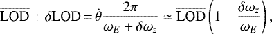
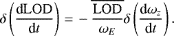
An offset δLOD of the length of day with respect to its nominal value is related to an equivalent variation, δω_z, of the angular velocity component with respect to ω_E, in such a way that $$\overline{\text{LOD}}+\delta \text{LOD}=\dot{\theta }\frac{2\pi }{{\omega }_E+\delta {\omega }_z}\simeq \overline{\text{LOD}}\left(1-\frac{\delta {\omega }_z}{{\omega }_E}\right),$$(1)

where the approximation sign stands for a first-order Taylor expansion in δω_z ∕ω_E, which is of small magnitude. Thus, the following relation is obtained (e.g. Wahr et al. 1981, or recently, Bizouard 2020), 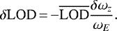$$\delta \text{LOD}=-\overline{\text{LOD}}\frac{\delta {\omega }_z}{{\omega }_E}.$$(2)

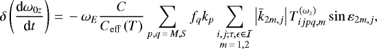
In this study we are interested in contributions to the secular angular acceleration of the Earth about its spin axis. The relation of this acceleration to the offsets of LOD time rate are then given by $$\delta \left(\frac{\text{dLOD}}{\text{d}t}\right)=-\overline{\frac{\text{LOD}}{{\omega }_E}}\delta \left(\frac{\text{d}{\omega }_z}{\text{d}t}\right).$$(3)

The structure of this paper is as follows. Section 2 summarizes the theoretical framework of the problem, explaining the main features of the canonical set of variables and the secular redistribution potential. The mathematical expressions are retrieved from previous works by the authors. In Sect. 3 the Earth’s rotation rate is studied, leading to the expression of the polar axis angular velocity component as a function of the canonical set under certain modeling assumptions. Following a perturbative procedure in the framework of generalized Hamiltonian systems in Sect. 4, an analytical closed-form expression for the Earth’s angular acceleration due to mass redistribution is obtained. In this formula, the anelastic response of the Earth is incorporated through frequency-dependent Love numbers, describing solid and oceanic tides. This section also includes a comparison with previous investigations – paying special attention to those incorporating similar modeling features – and with recent observational evidence of the phenomenon. Finally, Sect. 6 includes the conclusions of this work.

2 Secular redistribution potential in canonical variables

We take advantage of the previous works by Baenas et al. (2019, 2020a) to simplify the approach to the present research objective. An Andoyer-like set of canonical variables (Getino 1995) is used to describe the transformation between the non-rotating quasi-inertial reference system (OXYZ) and the Tisserand reference system of the Earth (Oxyz). This latter is referred to as a terrestrial system, and is defined as a reference system for the Earth’s mantle. The coordinates $\left\{\lambda ,\mu ,\nu \right\}$ and their conjugated momenta, $\left\{\Lambda ,M,N\right\}$, stand for the Andoyer variables of the Earth, while those of the fluid outer core (FOC) are denoted with a subscript c. Auxiliary angles, σ and I, are defined as functions of the canonical set through Λ = McosI and N = Mcosσ (giving the subtended angle of the angular momentum vector with the Earth’s figure axis and the Z axis of the non-rotating system, respectively). Similar relations with a subscript c define σ_c and I_c. A graphical description of these variables is shown in Fig. 1. The order of magnitude of σ and σ_c is about 10⁻⁶ rad (Kinoshita 1977; Getino 1995), which allows expansions of the functions of the canonical variables truncated in σ and σ_c. More details on these variables can be found in Baenas et al. (2017a) and references therein.

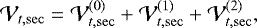
The redistribution potential energy, ${\mathcal{V}}_t$, is expressed in these Andoyer-like variables in the same way as the tidal (or tide-rasing) potential in the original Hamiltonian theory of the rigid Earth rotation (Kinoshita 1977). The method relies on an analytical solution of the ephemeris of the perturbers, and leads to a Fourier-like expansion of ${\mathcal{V}}_t$ where the secular part is identified by looking for the cancellation of the frequency of the trigonometric arguments. Baenas et al. (2019) can be consulted for further details on this procedure. Therefore, for purposes of this paper, we directly recover Eqs.(36) and (37) from this latter study, that is, the following expression of the secular redistribution potential, $${\mathcal{V}}_{t,\text{sec}}={\mathcal{V}}_{t,\text{sec}}^{(0)}+{\mathcal{V}}_{t,\text{sec}}^{(1)}+{\mathcal{V}}_{t,\text{sec}}^{(2)},$$(4)

where $$\begin{array}{lll}{\mathcal{V}}_{t,\text{sec}}^{(0)}\hfill & =\hfill & -\frac{9}{4}C{\omega }_E{\sum }_{p,q=M,S}{f}_q{k}_p{\sum }_{i,j;\tau ,ϵ\in \mathcal{I}}\left|{\overline{k}}_{20,j}\right|B_{i;p}{B}_{j;q}\hfill \\ \hfill & \hfill & \times \cos \left(\tau {\Theta }_i-ϵ{\Theta }_j-{\epsilon }_{20,j}\right),\hfill \\ {\mathcal{V}}_{t,\text{sec}}^{(1)}\hfill & =\hfill & -3C{\omega }_E{\sum }_{p,q=M,S}{f}_q{k}_p{\sum }_{i,j;\tau ,ϵ\in \mathcal{I}}\left|{\overline{k}}_{21,j}\right|C_{i;p}{C}_{j;q}\hfill \\ \hfill & \hfill & \times \cos \left(\mu +\nu -\tau {\Theta }_i-\tilde{\mu }-\tilde{\nu }+ϵ{\Theta }_j+{\epsilon }_{21,j}\right),\hfill \\ {\mathcal{V}}_{t,\text{sec}}^{(2)}\hfill & =\hfill & -\frac{3}{4}C{\omega }_E{\sum }_{p,q=M,S}{f}_q{k}_p{\sum }_{i,j;\tau ,ϵ\in \mathcal{I}}\left|{\overline{k}}_{22,j}\right|k_p{D}_{i;p}{D}_{j;q}\hfill \\ \hfill & \hfill & \times \cos \left(2\mu +2\nu -\tau {\Theta }_i-2\tilde{\mu }-2\tilde{\nu }+ϵ{\Theta }_j+{\epsilon }_{22,j}\right)\text{}.\hfill \end{array}$$(5)

In this expression, the (0), (1), and (2) superscripts stand for the zonal, tesseral, and sectorial components of the secular redistribution potential, respectively. Summation indices¹, i and j, represent the ith and jth orbital frequencies in the Fourier-like expansion of the orbital motion of the perturbed bodies (those gravitationally affected by the deformation of Earth) and the perturbing ones (those inducing the deformation of Earth via their gravitational field), respectively; τ and ϵ take the values ± 1 from certain linear combinations of the fundamental arguments Θ_i and Θ_j in the form τΘ_i − ϵΘ_j. The Moon (M) and the Sun (S) act at the same time as perturbing and perturbed bodies, and those two roles are distinguished using different notations. Namely, the perturbed bodies are identified with the set of indexes $\left\{i,p,\tau \right\}$, while $\left\{j,q,ϵ\right\}$ refers to theperturbers. This distinction is important because functions related to the perturbing bodies are time functions in our modeling, where the Earth’s rotational motion is decoupled from the orbital motion of the perturbers. In the same way, in order to distinguish the Andoyer variables corresponding to perturbed or perturbing bodies, the last ones are marked with a tilde symbol ($\tilde{\lambda }$, $\tilde{\mu }$, $\tilde{\nu }$, and Ĩ whose dependence is implicit in Eq. (5)), as in Getino & Ferrándiz (1995).

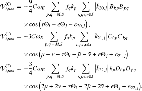
Modulus and phase of the complex Love functions are given by $\left|{\overline{k}}_{2m,j}\right|$ and ε_2m,j (m = 0, 1, 2). As the deformation is induced by the perturbers, these functions depend on the j index, namely on the jth orbital frequency inducing the anelastic response of the Earth. The ephemeris of the Moon and the Sun are included in the B_i;p, C_i;p, and D_i;p Kinoshita (1977) orbital functions (depending on auxiliary angle I), and their respective versions with j and q subscripts (depending on Ĩ) in the redistribution potential. As is customary, the polar principal moment of inertia of the Earth is represented by C. The k_p and f_q parameters are those of Kinoshita (1977) and Baenas et al. (2019), that is, $$k_p=\frac{3G{m}_p}{{\omega }_E{a}_p^2}{H}_d,f_q=\frac{m_q{a}_E^2}{3C{H}_d}{\left(\frac{a_E}{a_q}\right)}^3.$$(6)

Finally, the $\mathcal{I}$ set has been defined for the summation conditions, $$\mathcal{I}=\left\{\tau ,ϵ\in \{-1,+1\}\mid \tau {\Theta }_i-ϵ{\Theta }_j=0\right\},$$(7)

equivalent to the secular condition given by the cancelation of the frequency within the trigonometric arguments of the redistribution potential to obtain its ${\mathcal{V}}_{t,\text{sec}}$ portion.

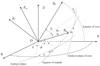Fig. 1 Andoyer-like canonical set for a two-layer Earth model.

3 Earth rotation rate in canonical variables

In the Oxyz Tisserand system of the deformable Earth, the elements of the matrix of inertia are functions of time. The inertia matrix can be decomposed in the form I = I₀ + I₁, where I₀ is a constant and diagonal matrix where the diagonal elements are given by the principal moments of inertia of the symmetric Earth, A = B< C, and I₁ is a time-varying symmetric matrix accounting for the tidal deformation of the Earth, and is small when compared with I₀. Specifically, the quotient between matrix elements of I₁ and C, I_1ij ∕C, are small parameters in the approximation of a first-order deformation (e.g. Escapa 2011; Getino & Ferrándiz 1995).

Moreover, I = I_m + I_c, where I_m and I_c are the inertia matrices of the mantle and core layers, respectively. We consider the angular velocity vector, ω, of the Oxyz system with respect to the OXYZ non-rotating one, and δω of the rotation of the geocentered core-fixed system with respect to the Tisserand one. The total angular momentum of the Earth (L) can therefore be decomposed into those of the mantle, L_m = I_mω, and the core, 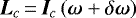$L_c=I_c\left(\omega +\delta \omega \right)$, as (Getino 1995; Moritz & Mueller 1986, Chap. 3) $$L=L_m+L_c=I\omega +I_c\delta \omega ,$$(8)

or, accordingly, the Earth’s angular velocity vector is given by 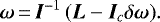$$\omega =I^{-1}\left(L-I_c\delta \omega \right)\text{}.$$(9)

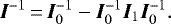
The matrix $I^{-1}={\left(I_0+I_1\right)}^{-1}$ can be expanded keeping only its first-order terms (in the order of magnitude of I_1ij ∕C) as $$I^{-1}=I_0^{-1}-I_0^{-1}{I}_1{I}_0^{-1}.$$(10)

Therefore, by considering Eqs. (9) and (10), the ω vector can be approximated by the following expansion $$\omega =I_0^{-1}L-I_0^{-1}{I}_1{I}_0^{-1}L-I^{-1}{I}_c\delta \omega .$$(11)

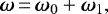
Here, the first two addends are those of a one-layer deformable Earth (Escapa 2011), which in turn are split into the angular velocity in the torque-free case ($I_0^{-1}L$) and the terms due to tidal perturbation ($-I_0^{-1}{I}_1{I}_0^{-1}L$), also known as convective terms (Efroimsky & Escapa 2007). The remaining part (− I⁻¹I_cδω) arises from the presence of the FOC in the two-layer Earth model. The core contribution can be expressed in a similar manner using a decomposition of I_c, as in that of I, namely I_c = I_c0 + I_c1, in such a way that $$\omega ={\omega }_0+{\omega }_1,$$(12)

where ω₀ comprises the torque-free terms, and ω₁ the convective terms collecting the tidal perturbation contributions, $$\begin{array}{lll}{\omega }_0\hfill & =\hfill & I_0^{-1}\left(L-I_{c0}\delta \omega \right),\hfill \\ {\omega }_1\hfill & =\hfill & -I_0^{-1}{I}_1{I}_0^{-1}\left(L-I_{c0}\delta \omega \right)-I_0^{-1}{I}_{c1}\delta \omega .\hfill \end{array}$$(13)

Here, it should be noted that second-order terms arising from the product of matrix elements of I₁ and I_c1 have been neglected in ω₁.

The convective terms play a key role in the study of the quasi-periodic evolution of ω, which is computed through the tidal kinetic energy of the system (e.g. Escapa 2011 for the one-layer elastic Earth case). However, they are negligible in a first-order theory when computing the secular evolution of ω, because it only emerges from the action of the redistribution potential. In fact, the increment of the rotational kinetic energy due to the Earth’s tidal deformation (${\mathcal{T}}_t$) has no secular part that can induce a secular contribution into the functions of the canonical variables when considering first-order perturbation equations. This is not the case for second-order terms in the sense of perturbation methods, where ${\mathcal{T}}_t$ has a non-negligible contribution, as is shown in Baenas et al. (2017a) for the case of precession in longitude. Further, the ${\mathcal{V}}_{t,\text{sec}}$ potential (Eq. (5)) is proportional to the dimensionless small parameters f_q (about 10⁻⁵, Baenas et al. 2019), while ω₁ terms are of order I_1ij∕C (about 10⁻⁴, Kubo 1991); the combination of both leads to a second-order contribution in the sense of magnitude.

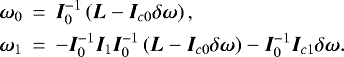
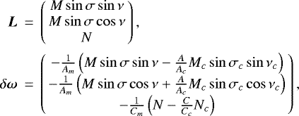
Therefore, in this investigation, we focus on the ω₀ angular velocity to obtain the Earth’s rotation rate in combination with the ${\mathcal{V}}_{t,\text{sec}}$ Hamiltonian through first-order perturbative equations. This objective requires writing the ω₀ third component, ω_0z, in the Andoyer-like canonical set, which is done by means of the L and δω respective expressions (e.g. Getino & Ferrándiz 1997), $$\begin{array}{lll}L\hfill & =\hfill & \left(\begin{array}{c}M\sin \sigma \sin \nu \\ M\sin \sigma \cos \nu \\ N\end{array}\right),\hfill \\ \delta \omega \hfill & =\hfill & \left(\begin{array}{c}-\frac{1}{A_m}\left(M\sin \sigma \sin \nu -\frac{A}{A_c}{M}_c\sin {\sigma }_c\sin {\nu }_c\right)\\ -\frac{1}{A_m}\left(M\sin \sigma \cos \nu +\frac{A}{A_c}{M}_c\sin {\sigma }_c\cos {\nu }_c\right)\\ -\frac{1}{C_m}\left(N-\frac{C}{C_c}{N}_c\right)\end{array}\right),\hfill \end{array}$$(14)

where A_m, A_c and C_m, C_c are the equatorial and polar principal moments of inertia of mantle and core, respectively. Performing the matrix operations in Eq. (13), and retaining only the third component of ω₀ vector, that is, the angular velocity about the polar axis in the terrestrial system, we obtain the following expression: $${\omega }_z\simeq {\omega }_{0z}=\frac{1}{C_m}\left(N-N_c\right)\text{}.$$(15)

With Eq. (15) we can calculate the secular deceleration of the Earth’s rotation due to tidal effects, which is given as an offset of the ω_0z time derivative (i.e. angular acceleration). Equation (15) is coincident with that of for example Getino (1995, Eq. (14)) which was obtained from the solution of the unperturbed Hamiltonian in a two-layer Earth model². However, using that method is not valid here because there is no consideration of the tidal mass redistribution, and therefore the convective terms do not appear. It should be noted that we strictly avoid the convective terms for numerical magnitude reasons in the case of the secular evolution of the Earth’s rotation rate, which is governed by the secular tidal redistribution potential.

4 Secular angular acceleration formula

4.1 Two-layer Earth with coupling torque at CMB

Following a parallel development such as that of the calculation of the precession rates in longitude and obliquity induced by the redistribution tidal potential (Baenas et al. 2019 can be consulted for details), this research is restricted to the study of the evolution of a given function of the canonical set under the secular perturbation Hamiltonian ${\mathcal{H}}_{\text{sec}}={\mathcal{V}}_{t,\text{sec}}.$ In particular, if ω_0z (Eq. (15)) is considered, its secular evolution is determined through the change of its time derivative, $\delta \left(\text{d}{\omega }_{0z}/\text{d}t\right)$, that is, secular angular acceleration. The applicable dynamical equation in the absence of dissipative torques comes from the Lie-Hori perturbation method (Hori 1966; Ferraz-Mello 2007), which is combined with an averaging method to isolate the secular evolution of the functions of the canonical set. At the first-order of perturbation, the equation $$\delta \left(\frac{\text{d}{\omega }_{0z}}{\text{d}t}\right)=\left\{{\omega }_{0z},{\mathcal{V}}_{t,\text{sec}}\right\}$$(16)

describes the secular evolution, where $\left\{-,-\right\}$ is the Poisson bracket³ expressed in terms of the Andoyer-like canonical variables. Taking into account the variables involved in ω_0z (Eq. (15)) and ${\mathcal{V}}_{t,\text{sec}}$ (Eq. (5)), the previous dynamical equation reduces to $$\delta \left(\frac{\text{d}{\omega }_{0z}}{\text{d}t}\right)=-\frac{1}{C_m}\frac{\partial {\mathcal{V}}_{t,\text{sec}}}{\partial \nu }.$$(17)

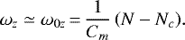
Equation (17) is similar to that of a one-layer Earth model, because there are no FOC variables. The reason for this is twofold: the ${\mathcal{V}}_{t,\text{sec}}$ potential ‘sees’ the Earth as a whole (Eq. (5) does not have core variables), and the dynamical equation (Eq. (17)) is a first-order perturbative one (at higher orders there are mixed terms with the generating functions of the method causing the presence of the core variables; e.g. Baenas et al. 2017a). However, this does not mean that the FOC has no influence on the secular angular acceleration at this approximation order. It must be noted that Eqs. (15) and (17) depend on the C_m mantle polar principal moment of inertia, while in a one-layer model the angular velocity is written as ω_0z = N∕C (Getino & Ferrándiz 1991), where C is the polar principal moment of inertia of the whole Earth. This difference between the one-layer and two-layer situations was also recognised by Yoder et al. (1981), who based their arguments on observational and rheological considerations, and its implications are discussed later.

However, Eq. (17) must be corrected in order to include the interaction between core and mantle due to the dissipative effects at the CMB, which can be incorporated into the Hamiltonian formalism of the two-layer Earth by means of the generalized forces approach (Getino & Ferrándiz 1997, 2001). This is the Hamiltonian counterpart of the Sasao et al. (1980) approach (known as SOS formalism and based on Euler–Liouville equations) to introduce a dissipative torque at the CMB accounting for electromagnetic coupling and viscosity. A modification of the Lie-Hori method in order to deal with a certain set of generalized Hamiltonian systems is exposed in Baenas et al. (2017b, 2020b). Such a modified Lie-Hori method is applicable here, and leads to the fact that the secular problem is not altered at the first order, except for the inclusion of the generalized forces within the auxiliary system (in our case, the unperturbed situation).

We are particularly interested in the third component of the dissipative torque acting on the core in the Tisserand system, − R^*δω₃, where R^* is a coupling constant following the notation of Getino & Ferrándiz. When dealing with generalized canonical systems, the time evolution of a function of the canonical set not only depends on the Hamiltonian at the first-order of perturbation (Eq. (16)) but also on the generalized forces. An explanation of the fundamentals of this type of mechanical system can be found in Escapa (2006, Sect. 1.2.1). Briefly, the time evolution of a smooth f function of the $\left(q,p\right)$ canonical set in a generalized canonical system is given by $$\frac{\text{d}}{\text{d}t}f=\left\{f,\mathcal{H}\right\}+\frac{\partial f}{\partial t}-{\sum }_{i=1}^n\left(\frac{\partial f}{\partial q_i}{Q}_{p_i}-\frac{\partial f}{\partial p_i}{Q}_{q_i}\right),$$

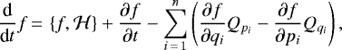
where $\mathcal{H}$ is the Hamiltonian of the system, and $Q_{p_i}$ and $Q_{q_i}$ the generalized forces.. In our case, ω_0z depends on N and N_c variables (Eq. (15)), whose secular evolution in a two-layer model incorporating mass redistribution is governed by the following equations at first order in σ and σ_c, 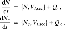$$\begin{array}{lll}\frac{\text{d}N}{\text{d}t}\hfill & =\hfill & \left\{N,V_{t,\text{sec}}\right\}+Q_{\nu },\hfill \\ \frac{\text{d}{N}_c}{\text{d}t}\hfill & =\hfill & \left\{N_c,V_{t,\text{sec}}\right\}+Q_{{\nu }_c}.\hfill \end{array}$$(18)

Here, Q_ν and $Q_{{\nu }_c}$ are the generalized forces corresponding to the ν and ν_c coordinates (N and N_c being their conjugated momenta) obtained from the coupling torque. Their construction can be retrieved from Getino & Ferrándiz (1997). The Q_ν force is null because the virtual work of the torque only depends on the virtual displacement of the core variables, while $Q_{{\nu }_c}$ is given by 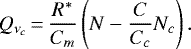$$Q_{{\nu }_c}=\frac{R^{\ast }}{C_m}\left(N-\frac{C}{C_c}{N}_c\right).$$(19)

It must be noted that the decoupled situation is recovered if R^* = 0, but also if the free–torque approximations N ≃ Cω_E and N_c ≃ C_cω_E are taken (usually employed for numerical estimates), both leading to $Q_{{\nu }_c}=0$. Equation (18) is simplified because $\left\{N_c,V_{t,\text{sec}}\right\}$ vanishes. Meanwhile, $\left\{N,V_{t,\text{sec}}\right\}=$ $-\partial {\mathcal{V}}_{t,\text{sec}}/\partial \nu$ can be evaluated at some epoch (J2000.0) for our purposes, giving a constant value, as is shown in the following section. Therefore, Eq. (18) is equivalent to the following second-order linear differential equation with constant coefficients in the canonical momentum N_c, 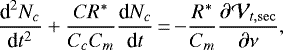$$\frac{{\text{d}}^2{N}_c}{\text{d}{t}^2}+\frac{C{R}^{\ast }}{C_c{C}_m}\frac{\text{d}{N}_c}{\text{d}t}=-\frac{R^{\ast }}{C_m}\frac{\partial {\mathcal{V}}_{t,\text{sec}}}{\partial \nu },$$(20)

$C{R}^{\ast }/\left(C_m{C}_c\right)$ being the damping coefficient. The solution of the initial value problem given by Eq. (20) and the initial conditions $N_c\left(0\right)$ and $\left(\text{d}{N}_c/\text{d}t\right)\left(0\right)=0$, by standard procedure, allows us to write, taking into account Eq. (15), $$\frac{\text{d}}{\text{d}t}\left(\frac{N-N_c}{C_m}\right)=-\frac{1}{C}\left(1+\frac{C_c}{C_m}{e}^{-\frac{C{R}^{\ast }t}{C_m{C}_c}}\right)\frac{\partial {\mathcal{V}}_{t,\text{sec}}}{\partial \nu }.$$(21)

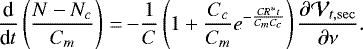
Therefore, the secular evolution of dω_0z∕dt is given by the time-averaging of Eq. (21) over a T period of time. For the sake of convenience, we define 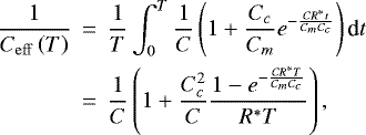$$\begin{array}{lll}\frac{1}{C_{\text{eff}}\left(T\right)}\hfill & =\hfill & \frac{1}{T}{\displaystyle {\int }_0^T\frac{1}{C}}\left(1+\frac{C_c}{C_m}{e}^{-\frac{C{R}^{\ast }t}{C_m{C}_c}}\right)\text{d}t\hfill \\ \hfill & =\hfill & \frac{1}{C}\left(1+\frac{C_c^2}{C}\frac{1-e^{-\frac{C{R}^{\ast }T}{C_m{C}_c}}}{R^{\ast }T}\right),\hfill \end{array}$$(22)

where $C_{\text{eff}}\left(T\right)$ is a time function playing the role of the time-averaged effective inertia moment. In the previous integral, t = 0 formally stands for the initial moment of the actuation of the dissipative torque, where only the T elapsed time of evolution is relevant. Equations (21) and (22) allow us to write 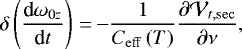$$\delta \left(\frac{\text{d}{\omega }_{0z}}{\text{d}t}\right)=-\frac{1}{C_{\text{eff}}\left(T\right)}\frac{\partial {\mathcal{V}}_{t,\text{sec}}}{\partial \nu },$$(23)

which generalizes Eq. (17) for the secular angular acceleration of the Earth over a period of time T because of the redistribution potential effects and when a dissipative core–mantle coupling torque is introduced within the modeling⁴.

Equation (17), which describes the secular evolution of the Earth’s rotation rate when the FOC and the mantle evolve decoupled, is obtained from Eq. (23) in the limiting case of a null period of core–mantle coupling, that is, $C_{\text{eff}}\left(0\right)\equiv \underset{T\to 0}{\lim }{C}_{\text{eff}}\left(T\right)=C_m$. Such physical behavior of the decoupled FOC in the rotation of Earth is studied in Wahr et al. (1981), Yoder et al. (1981), and Moritz & Mueller (1986), Sect. 3.7, among others.

In turn, if the core–mantle coupling is prolonged indefinitely in time, we have $C_{\text{eff}}\left(\infty \right)\equiv \underset{T\to \infty }{\lim }{C}_{\text{eff}}\left(T\right)=C$. Because in this case Eq. (23) is equivalent to that of a one-layer deformable Earth model (where ω_0z = N∕C), the introduction of dissipative effects through a coupling torque at the CMB implies a limit situation in the secular evolution of the angular acceleration where the two-layer Earth behaves as a whole, with core and mantle decelerating together. This property is due to the fact that dissipative coupling tends to attenuate the differential rotation between core and mantle. With respect to the redistribution potential perturbation, a one-layer deformable Earth is indistinguishable from a two-layer Earth with totally coupled core and mantle. The core–mantle total coupling in the secular evolution – $C_{\text{eff}}\left(\infty \right)$ – is assumed from the outset by example Mathews & Lambert (2009) or Williams & Boggs (2016), although such an assumption is not justified in those studies.

4.2 Secular angular acceleration due to mass redistribution

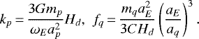
Once the derivative in Eq. (23) is performed, it is possible to identify the sets of variables of perturbed and perturbing bodies, that is, $\tilde{\lambda }=\lambda$, $\tilde{\mu }=\mu$, and $\tilde{\nu }=\nu$, because they are the same bodies but play different mathematical roles in ${\mathcal{V}}_{t,\text{sec}}$. The secular condition (Eq. (7)) must therefore be applied. The B, C, and D Kinoshita orbital functions can be evaluated with sufficient accuracy at some epoch, that is, I = Ĩ = I₀ (J2000.0), taking into account the fact that the value of such functions does not vary substantially throughout the integration period. Further minor details from a similar calculation can be found in Baenas et al. (2017a, 2019). Finally, the contribution to the secular angular acceleration, or Earth rotation rate, reads $$\delta \left(\frac{\text{d}{\omega }_{0z}}{\text{d}t}\right)=-{\omega }_E\frac{C}{C_{\text{eff}}\left(T\right)}{\sum }_{p,q=M,S}{f}_q{k}_p{\sum }_{\begin{array}{c}i,j;\tau ,ϵ\in \mathcal{I}\\ m=1,2\end{array}}\left|{\overline{k}}_{2m,j}\right|T_{ijpq,m}^{\left({\omega }_z\right)}\sin {\epsilon }_{2m,j},$$(24)

where the following orbital-dependent function has been defined: 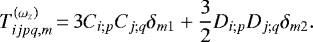$$T_{ijpq,m}^{\left({\omega }_z\right)}=3C_{i;p}{C}_{j;q}{\delta }_{m1}+\frac{3}{2}{D}_{i;p}{D}_{j;q}{\delta }_{m2}.$$(25)

In Eq. (25), δ_mn stands for Kronecker delta symbol, introduced by the dependence of the Love number set with m index of thefrequency band. As there is no contribution of the zonal part of the redistribution potential, because $\partial {\mathcal{V}}_{t,\text{sec}}^{(0)}/\partial \nu =0$, the m index in Eq. (24) only counts for m = 1, 2.

The dimensionless $C/C_{\text{eff}}\left(T\right)$ quotient establishes the type of core–mantle evolution considered during a period of time where $C_{\text{eff}}\left(T\right)$ acts as the time-averaged moment of inertia. The theoretical situation of a decoupled core–mantle secular evolution is studied by taking 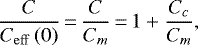$$\frac{C}{C_{\text{eff}}\left(0\right)}=\frac{C}{C_m}=1+\frac{C_c}{C_m},$$(26)

where the unit part corresponds to the one-layer Earth case, while C_c ∕C_m works as the contribution due to the two-layer modeling. The widespread assumption (Mathews & Lambert 2009; Williams & Boggs 2016) is the totally coupled core–mantle secular evolution, which is given by $$\frac{C}{C_{\text{eff}}\left(\infty \right)}=\frac{C}{C}=1.$$(27)

5 Numerical results and comparisons

A numerical estimate of the exponential in Eq. (22) can be performed considering the frictional coupling constant magnitude, R^* ≃ 3.2 × 10²⁸ kg m² s⁻¹ (Stacey & Davis 2008, Sect. 7.5), and numerical values of the principal inertia moments (e.g., Chen et al. 2015). The exponential shows a fast decay (~e^−12.6T, T in cy), allowing its numerical irrelevance in a few centuries. Hence, in what follows, totally coupled core–mantle secular evolution is assumed (Eq. (27)).

For the numerical evaluation of Eq. (24) we use the IERS Conventions (IERS Conventions 2010) frequency-dependent Love number set for solid tides (with oceanic load), and Williams & Boggs (2016) correction to account for the direct contribution of the oceans based on the FES2004 (Lyard et al. 2006) ocean tide model. In addition to those references, Baenas et al. (2019) can be consulted for further details on such Love number sets. This is a very complete scenario to describe the Earth’s anelastic response to gravitational perturbation, which is integrated in the formula through the modulus and phase, $\left|{\overline{k}}_{2m,j}\right|$ and ε_2m,j (m = 1, 2), of the complex Love numbers. We use the same sign convention for the ε_2m,j phase as that used in Williams & Boggs (2016).

The rest of the involved parameters are those of Table 1 in Baenas et al. (2019) (not included here for the sake of brevity), and the factor 1 + C_c∕C_m (Eq. (26)) used for comparative purposes. A numerical estimate of 1 + C_c∕C_m can be obtained from the basic Earth parameters (BEPs) of the two-layer Earth (Getino & Ferrándiz 2001), namely P_CW (period of Chandler wobbe), P_FCN (period of free core nutation), and the A_c∕A_m ratio, which are connected through the ellipticities of the Earth (e) and the FOC (e_c); or with a direct calculation of the C_c∕C_m ratio following for example Chen et al. (2015). In any case, the approximation C_c ∕C_m ≃ A_c∕A_m can be accepted with great accuracy⁵, and therefore we take 1 + C_c∕C_m ≃ 1.1284 (with A_c∕A_m given by Dziewonski & Anderson 1981). In other words, Eq. (24) directly shows that the influence of the decoupled FOC in the angular deceleration of the rotation of Earth about its spin axis is about 11% in magnitude (in agreement with Wahr et al. 1981)⁶.

Table 1 displays the numerical contributions obtained from Eq. (24) divided into tides and Earth modeling situations. In Table 2, the division is made according to frequency band or harmonic contribution of the redistribution potential, that is, tesseral (m = 1, diurnal) and sectorial (m = 2, semidiurnal), in the coupled core–mantle secular evolution. Both tables show the results in angular acceleration (arcseconds/century², ′′ cy⁻²) and LOD rate (millisecond/century, ms cy⁻¹, ms are implicitly per day), computed through Eq. (3).

In coupled core–mantle secular evolution, the total contribution of the secular redistribution potential in the deformable two-layer Earth with oceans is given by an angular acceleration of − 1328.6′′ cy⁻² (secular deceleration), equivalent to 2.418 ms cy⁻¹ in the LOD rate. This result is mainly due to the ocean tides (Table 1), and the semidiurnal band of the redistribution potential (Table 2). Regarding the separate action of each perturber, the Moon induces a deceleration of − 1135.3′′ cy⁻² (2.067 ms cy⁻¹, 85.45%), while the Sun contributes − 193.3′′ cy⁻² (0.352 ms cy⁻¹, 14.55%).

Some comparisons with previous works on the calculation of the secular deceleration are included in Table 3. Here, AE and OT labels refer to the anelasticity of the mantle and the oceanic tide, respectively. The value given by Getino & Ferrándiz (1991) is obtained with a one-layer Earth model using the Hamiltonian formalism. These authors introduce ad hoc phases per frequency band in the trigonometric arguments to account for the anelastic behavior in the Earth deformation. Equation (40) in this latter paper is somehow equivalent to our Eqs. (24) and (25) for the case of a one-layer Earth with a constant Love number. These simplifications lead to an LOD rate that is lower than ours by about 0.32 ms cy⁻¹. Krasinsky (1999) uses a similar Earth modeling to that of Getino & Ferrándiz (1991) but in the framework of Newtonian mechanics. The obtained results are very close in both approaches.

In Ray et al. (1999), the obtained LOD rate is only due to ocean tides based on satellite-altimeter and satellite-tracking tide solutions. The formalism used by these latter authors does not provide an analytical formula, and so the comparison is strictly numerical. The suitable comparison must be partial with respect to our total values in the ocean tides column of Table 2. This leads to a small increase in LOD rate of about 0.07 ms cy⁻¹.

5.1 Comparison with Mathews & Lambert (2009)

Lambert & Mathews (2008) and Mathews & Lambert (2009) make very similar theoretical assumptions to those made in this investigation. We focus on the latter study as it is an update of the former on the same topic. In Mathews & Lambert (2009), a two–layer Earth model with oceanic contribution is tackled within the SOS approach. As in our construction, terms of second order in magnitude are considered to be negligible, avoiding the effect of the differential rotation of the core. The coupled core–mantle secular evolution is assumed by these authors from the outset. Due to the fact that the employed formalism does not provide analytical results, the comparison is also strictly numerical.

Table 1 of Mathews & Lambert (2009) is directly comparable to Table 2 of this work, both giving an angular acceleration and LOD rate split in the harmonic components of the tidal potential. There is a typo in Table 1 of this latter work: the total amount of the angular acceleration is − 1369 ′′ cy⁻² (instead of the stated − 1449′′ cy⁻²), corresponding to 2.50 ms cy⁻¹ in the LOD rate. In the total count, there is a small difference with respect to our calculation of about + 40′′ cy⁻² or an increase of 0.08 ms cy⁻¹, mostly coming from the ocean tides contribution.

Furthermore, there are substantial differences between the oceanic model used by Lambert & Mathews (2006, 2008), which is the supporting theory of Mathews & Lambert (2009), and that of Williams & Boggs (2016), which is included in our calculations (this topic was already discussed in Baenas et al. 2020a). In addition, in Mathews & Lambert (2009) the Earth’s mantle anelasticity and oceanic contribution are tackled by means of constant compliances (parameters proportional to Love numbers) defined per frequency band, which is a simplification with respect to the more realistic situation of frequency-dependent tidal deformation (Love functions) used in our approach. Table 4 shows that such a simplification explains the differences found in the solid tides contributions. In Table 4 we use constant Love numbers per frequency band in Eq. (24), i.e., ${\overline{k}}_{2m,j}={\overline{k}}_{2m}$, taken from Table 6.3 of IERS Conventions (2010). The angular acceleration and LOD rate contributions are compared with their counterparts in Table 1 of Mathews & Lambert (2009), displayed in parentheses in the table. Both sets of numerical results are in good agreement.

5.2 Comparison with Williams & Boggs (2016)

The calculation of the Earth rotation rate in Williams & Boggs (2016) is performed through evaluation of the torque acting to decelerate the rotation of the Earth about its polar axis following an analytical approach in an assumed coupled core–mantle secular evolution situation. The same orbital ephemeris solution for the perturbers (ELP2000, Chapront-Touzé & Chapront 1983) is used as thatof the Hamiltonian formalism (Kinoshita and Souchay 1990) adopted in this work. After some algebra it can be shown that Eq. (26) of Williams & Boggs (2016) is equivalent to our Eq. (5) of the redistribution tidal potential⁷. Accordingly,this coincidence also happens with their Eq. (28) of the tidal angular acceleration and Eqs. (24) and (25) of the present paper, in the totally coupled core–mantle case. In view of the fact that we have used the Williams & Boggs (2016) Love number set of the Earth with oceans, we expect to see very good agreement in the numerical results of both investigations.

As shown in Table 3, Williams & Boggs (2016) give a secular contribution of − 1316′′ cy⁻² to the angular acceleration, corresponding to 2.40 ms cy⁻¹ in the LOD rate. This is a difference of about − 13′′ cy⁻² and 0.02 ms cy⁻¹ with respect to our values (Table 1), respectively. These differences are further reduced to − 6′′ cy⁻² and 0.01 ms cy⁻¹ if we consider the S_W = 1.005 parameter introduced ad hoc in Eq. (28) of Williams & Boggs (2016) to take into account the small dependence of the C moment of intertia on spin rate, i.e., a direct substitution of C with S_WC. These almost negligible differences can only be attributed to small changes in the constants used in the modeling.

5.3 Comparison with observational evidence

The secular angular acceleration of the Earth is an average magnitude consisting of tidal contributions (solid, oceanic, and atmospheric tides) and other parts of nontidal origin inducing a secular change in the Earth’s oblateness or inertia matrix. The most important of these nontidal geophysical effects is the glacial isostatic adjustment (GIA) attributed to viscous rebound of the solid Earth from the decrease in load on the polar caps following the last deglaciation (Peltier & Wu 1983; Yoder et al. 1983; Williams et al. 2016). Mechanisms linked to the core–mantle coupling (Mitrovica et al. 2009) and some other identified sources producing a linear trend in LOD (a list of them can be found in Gross 2015) are also taken into account.

The average value of the LOD rate can be estimated in different ways from observational methods, some of them depending on ancient astronomical observations. This is the case of the study of Stephenson et al. (2016), which is based on a previous work by Stephenson & Morrison (1995), where the authors consider reports of solar and lunar eclipses between 720 BC and AD 2015. In Stephenson et al. (2016), the average change in the LOD with tidal origin is obtained following an empirical relation between the observed tidal acceleration of the Moon and the retardation of the Earth’s spin due to lunar and solar tides (Christodoulis et al. 1988). Stephenson et al. (2016) estimate an increase of 2.3 ± 0.1 ms cy⁻¹ in LOD due to tidal friction, which is consistent with their averaged observed change of 1.78 ± 0.03 ms cy⁻¹ (including effects of tidal and nontidal origin). In order to perform a proper comparison of this value with our theoretical prediction, it is interesting to note that Ray et al. (1999) give a contribution of the atmospheric tides, amounting to an angular acceleration of + 55′′ cy⁻². Assuming this complementary tidal contribution, our complete estimate for comparative purposes gives a secular acceleration of − 1273.6′′ cy⁻², or 2.32 ms cy⁻¹ of LOD rate offset: this is a relative error of less than 0.9% with respectto that of Stephenson et al. (2016).

Morrison et al. (2021) is a recent update of the work by Stephenson et al. (2016). However, in this addendum the authors have taken the tidal part of the LOD rate from Williams & Boggs (2016), namely 2.40 ms cy⁻¹. As such an estimate comes from a calculation similar to that of the present paper (we make the comparison with Williams & Boggs 2016 in Sect. 5.2), it does not provide relevant information in terms of observational evidence of the tidal offset in LOD. The updated value of the observed deceleration is 1.72 ± 0.03 ms cy⁻¹ (including effects of tidal and nontidal origin). As pointed out above, the widespread assumption explaining the substantial difference between the predicted change of the LOD rate with tidal origin and the observed one is mainly ascribed to GIA. Mitrovica & Forte (1997) found that GIA causes a secular trend in LOD of − 0.5 ms cy⁻¹ (Gross 2015), which is in very good agreement with the difference of − 0.5 ms cy⁻¹ for the nontidal contribution found by Stephenson et al. (2016), and even the updated value of − 0.7 ms cy⁻¹ in Morrison et al. (2021).

It is interesting to note that, prior to these estimates, Christodoulis et al. (1988) gave an observed tidal braking of the Earth’s rotation rate of 2.24 ± 0.08 ms cy⁻¹ (− 5.98 ± 0.22 × 10⁻²² rad s⁻² in the original paper) based on laser and Doppler range data from artificial satellites. With respect to the center of the interval, the relative difference with our calculation is less than 3.5%, the 2.32 ms cy⁻¹ being included in the interval error. Their value has been confirmed by Deines & Williams (2016) by means of an indirect empirical method based on fossil data. This investigation leads to a very close average value of despinning rate, 2.23 ± 0.66 ms cy⁻¹ (− 5.969 ± 1.762 × 10⁻²² rad s⁻² in the original paper). However, due to the large error interval affecting their inferred LOD rate, all the theoretical predictions in Table 3 are covered.

Regardless of the set of geophysical effects causing changes in the Earth’s oblateness, the decrease of the polar principal moment of inertia C has been monitored for several decades using methods of satellite geodesy, showing a decreasing trend (Rubincam 1982; Cox & Chao 2002; Cheng et al. 2013) and periodic components (Marchenko 2018). In this sense, it should be noted that the derivation of our formula for the secular angular acceleration due to tidal mass redistribution (Eq. (24)) assumes the C, C_c, and C_m moments of inertia as constants. This working hypothesis avoids the inclusion of the nontidal change in the Earth’s oblateness within the modeling, allowing us to isolate the tidal contribution as required for the purposes of this investigation. It can be proven that tidal and nontidal parts of the secular LOD rate are decoupled at first order when only the linear trend is considered. The investigation of such nontidal effects on LOD within the Hamiltonian framework is an interesting topic, and one that we aim to investigate in future work.

6 Conclusions

In this work we use the Hamiltonian formalism of Earth rotation theory to derive a closed-analytical formula comprising the contribution of the secular redistribution potential to the angular acceleration in the rotation rate. The formula can be evaluated for different Earth rheological and oceanic models by means of frequency-dependent Love number formalism. We compare our numerical results with previous works in detail, and explain existing discrepancies.

We study the secular evolution of the Earth rotation rate, including the dissipative torque at the CMB. We describe such core–mantle coupling by means of a generalized forces approach and use the first-order Lie-Hori perturbation method combined with an averaging method. Within this framework, we define a time-averaged effective moment of inertia $C_{\text{eff}}\left(T\right)$, which comprises the limit situations of core–mantle decoupled evolution, and the situation where core and mantle are rigidly connected in their secular evolution or response to the long-term perturbations.

Our best estimate is achieved for a two-layer Earth model composed of an anelastic mantle with oceans and fluid outer core. Solid tides with ocean load are described through IERS Conventions (2010) frequency-dependent Love numbers, while oceans tides are introduced following Williams & Boggs (2016). With this Earth modeling, we obtain a secular angular acceleration of − 1328.6′′ cy⁻² (deceleration) equivalent to an increase in the LOD rate of 2.418 ms cy⁻¹. We show that such an estimate is in very good agreement with a recent determination of the Earth’s tidal braking (Williams &Boggs 2016; Stephenson et al. 2016) and is consistent with the total rates inferred from observations (Morrison et al. 2021). The main components of this result are the ocean tides and the semidiurnal band or sectorial component of redistribution potential. With respect to the perturbers, the Moon induces 85.45% of the secular deceleration.

This paper is the third in a series studying the effects of the mass redistribution potential on the rotation of the Earth, namely, Baenas et al. (2019; precession), Baenas et al. (2020a; nutation), and the present paper (secular changes in the length of day). All these results have been obtained taking advantage of the versatility of the Hamiltonian approach, which allows not only the numerical estimates without consistency problems (Escapa et al. 2017), but the achievement of analytical formulae describing the physical effects. The canonical framework also allows second-order effects to be dealt with; strictly speaking these cannot be studied with linear-based theories (Escapa et al. 2020). In this way, within the general scope of the mass redistribution effect, Baenas et al. (2017a) can also be included in the same list, where the influence of mantle elasticity on precessional motion in longitude is studied through a second-order effect in the sense of perturbation methods. The final report of the International Astronomical Union (IAU) and International Association of Geodesy (IAG) Joint Working Group on the theory of Earth rotation and validation (Ferrándiz et al. 2020), and Resolution 5 adopted⁸ by the IAG General Assembly in 2019, include some of the theoretical recommendations and updated values of Earth rotation parameters belonging to this series of works.

Acknowledgements

The authors thanks the anonymous referee for their useful comments. This research has been developed within the framework of the IAU/IAG Joint Working Group 3.1: Improving Theories and Models of the Earth’s Rotation (ITMER).

References

All Tables

All Figures

	Fig. 1 Andoyer-like canonical set for a two-layer Earth model.
In the text

References

- Baenas, T., Ferrándiz, J. M., Escapa, A., Getino, J., & Navarro, J. F. 2017a, AJ, 153, 79 [Google Scholar]
- Baenas, T., Escapa, A., Ferrándiz, J. M., & Getino, J., 2017b, Int. J. Nonlinear Mech., 90, 11 [Google Scholar]
- Baenas, T., Escapa, A., & Ferrándiz, J. M., 2019, A&A, 626, A58 [CrossRef] [EDP Sciences] [Google Scholar]
- Baenas, T., Escapa, A., & Ferrándiz, J. M., 2020a, A&A, 643, A159 [EDP Sciences] [Google Scholar]
- Baenas, T., Escapa, A., & Ferrándiz, J. M., 2020b, Adv. Space Res., 66, 2646 [Google Scholar]
- Bizouard, C. 2020, Geophysical Modelling of the Polar Motion (Germany: De Gruyter, Berlin & Boston) [Google Scholar]
- Chapront-Touzé, M., & Chapront, J. 1983, A&A, 124, 50 [NASA ADS] [Google Scholar]
- Chen, W., Li, J. C., Ray, J., Shen, W. B., & Huang, C. L. 2015, J. Geodyn., 89, 179 [Google Scholar]
- Cheng, M., Tapley, B. D., & Ries, J. C. 2013, J. Geophys. R. Solid Earth, 118, 740 [Google Scholar]
- Christodoulidis, D. C., Smith, D. E., Williamson, R. G., & Klosko, S. M. 1988, J. Geophys. Res., 93, 6216 [Google Scholar]
- Cox, C. M., & Chao, B. F. 2002, Science 297, 5582, 831 [Google Scholar]
- Deines, S. D., & Williams, C. A. 2016, AJ, 151, 103 [Google Scholar]
- Dziewonski, A. M., & Anderson, D. L. 1981, Phys. Earth Planet. Int., 25, 297 [Google Scholar]
- Efroimsky, M., & Escapa, A. 2007, Celest. Mech. Dyn. Astron., 98, 251 [Google Scholar]
- Escapa, A. 2006, PhD Thesis, University of Alicante, Alicante, Spain [Google Scholar]
- Escapa, A. 2011, Celest. Mech. Dyn. Astron., 110, 99 [Google Scholar]
- Escapa, A., Getino, J., Ferrándiz, J. M., & Baenas, T. 2017, A&A, 604, A92 [NASA ADS] [CrossRef] [EDP Sciences] [Google Scholar]
- Escapa, A., Getino, J., Ferrándiz, J. M., & Baenas, T. 2020, in Proc. Journées “Systèmes de Référence Spatio-temporels” 2019, ed. C. Bizouard (Observatoire de Paris), 221, https://syrte.obspm.fr/astro/journees2019/FILES/escapa.pdf [Google Scholar]
- Ferrándiz, J. M., Gross, R. S., Escapa, A., et al. 2020, International Association of Geodesy Symposia (Berlin: Springer) [Google Scholar]
- Ferraz-Mello, S. 2007, Canonical Perturbation Theories: Degenerate Systems and Resonance (New York: Springer) [Google Scholar]
- Getino, J. 1995, Geophys. J. Int., 122, 803 [Google Scholar]
- Getino, J., & Ferrándiz, J. M. 1991, Celest. Mech. Dyn. Astron., 52, 381 [Google Scholar]
- Getino, J., & Ferrándiz, J. M. 1995, Celest. Mech. Dyn. Astron., 61, 117 [Google Scholar]
- Getino, J., & Ferrándiz, J. M. 1997, Geophys. J. Int., 130, 326 [Google Scholar]
- Getino, J., & Ferrándiz, J. M. 2001, MNRAS, 322, 785 [Google Scholar]
- Gross, R. S. 2015, Physical Geodesy: Treatise on Geophystics, Earth Rotation Variations (Oxford: Elsevier), 3.09, 215 [Google Scholar]
- Hori, G. I. 1966, PASJ 18, 287 [Google Scholar]
- IERS Conventions 2010, IERS Technical Note 36, eds. G. Petit, & B. Luzum, 179 [Google Scholar]
- Kinoshita, H. 1977, Celest. Mech. Dyn. Astron., 15, 277 [Google Scholar]
- Kinoshita, H., & Souchay, J. 1990, Celest. Mech. Dyn. Astron., 48, 187 [Google Scholar]
- Krasinsky, G. A. 1999, Celest. Mech. Dyn. Astron., 75, 39 [Google Scholar]
- Kubo, Y. 1991, Celest. Mech. Dyn. Astron., 50, 165 [Google Scholar]
- Lambert, S. B., & Mathews, P. M. 2006, A&A, 453, 363 [NASA ADS] [CrossRef] [EDP Sciences] [Google Scholar]
- Lambert, S. B., & Mathews, P. M. 2008, A&A, 481, 883 [NASA ADS] [CrossRef] [EDP Sciences] [Google Scholar]
- Lyard, F., Lefevre, F., Letellier, T., & Francis, O. 2006, Ocean Dyn., 56, 394 [Google Scholar]
- Marchenko, A. N. 2018, Geodynamics, 2, 5 [Google Scholar]
- Mathews, P. M., & Lambert, S. B. 2009, A&A, 493, 325 [EDP Sciences] [Google Scholar]
- Mitrovica, J. X., & Forte, A. M. 1997, J. Geophys. Res., 102, B2, 2751 [Google Scholar]
- Mitrovica, J., Hay, C., Morrow, E., et al. 2015, Sci. Adv., 1, E1500679 [Google Scholar]
- Moritz, H., & Mueller, I. 1986, Earth Rotation (New York: Frederic Ungar) [Google Scholar]
- Morrison, L. V., Stephenson, F. R., Hohenkerk, C. Y., & Zawilski, M. 2021, Proc. R. Soc. A, 477, 20200776 [Google Scholar]
- Munk W. K., & MacDonald, G. J. F. 1960, The Rotation of the Earth: a Geophysical Discussion (Cambridge: Cambridge University Press) [Google Scholar]
- Peale, S. J. 1973, Rev. Geophys. Space. Phys., 11, 767 [Google Scholar]
- Peltier, W. R., & Wu, P. 1983, Geophys. J. R. Astron. Soc., 74, 377 [Google Scholar]
- Ray, R. D., Bruce, G. B., & Chao, B. F. 1999, J. Geophys. Res., 104, 17653 [Google Scholar]
- Rubincam, D. P. 1982, Celest. Mech., 26, 361 [Google Scholar]
- Sasao, T., Okubo, S., & Saito, M. 1980, Proc. IAU Symp., 78, 165 [Google Scholar]
- Stacey, F. D, & Davis, P. M. 2008, Physics of the Earth (New York: Cambridge University Press) [Google Scholar]
- Stephenson, F. R., & Morrison, L. V. 1995, Phil. Trans. R. Soc. London A., 351, 165 [Google Scholar]
- Stephenson, F. R., Morrison, L. V., & Hohenkerk, C. Y. 2016, Proc. R. Soc. A, 472, 160404 [Google Scholar]
- Wahr, J. M., Sasao, T., & Smith, M. L. 1981, Geophys. J. R. Astron. Soc., 64, 635 [Google Scholar]
- Williams, J. G., & Boggs, D. H. 2016, Celest. Mech. Dyn. Astron., 126, 89 [Google Scholar]
- Williams, J. G., Turyshev, S. G., & Boggs, D. H. 2014, Planet. Sci., 3, 2 [Google Scholar]
- Yoder, C. F., Williams, J. G., & Parke, M. E. 1981, J. Geophys. Res., 86, 881 [Google Scholar]
- Yoder, C. F., Williams, J. G., Dickey, J. O., et al. 1983, Nature, 303, 757 [Google Scholar]
The summation index i (and j) is an abridged notation of a quintuple of integers, mki (k = 1, 2, …, 5), such that the fundamental argument Θi (and Θj) is given by Θi = m1il + m2il′ + m3iF + m4iD + m5iΩ, where l, g, and h are the Delaunay variables of the Moon, l′, g′, and h′ are those of the Sun, and F = l + g, D = l + g + h − l′− g′− h′, and Ω = h − λ (Kinoshita 1977).
In the Hamiltonian approach of Getino & Ferrádiz, which is based on the Lie–Hori perturbation method, the unperturbed problem of a two-layer Earth is shared by the Poincaré model (rigid mantle and FOC, Getino 1995), or the cases including the
(Getino & Ferrándiz 2001) and
(Baenas et al. 2019, 2020a) tidal perturbations.
The Poisson bracket (or Lie derivative) of two f
and g smooth functions of the  canonical set is defined by the bilinear operation
The same result is achieved if Eq. (16) is generalized by
Depending on the selected Earth set of parameters, the relative error between Ac ∕Am and Cc ∕Cm can vary from 5 ppm to 0.1%.
The combination of Eqs. (2.8) and (2.10) in Wahr et al. (1981) lead to such a result because the numerical value of the ratio between LOD offsets in the cases of the Earth with FOC and the entirely solid Earth is given by 0.886. In our case, C∕Cm ≃ 0.886. This fact is also stated in Moritz & Mueller (1986; Sect. 3.7).
Such a comparison requires the relation between Williams & Boggs (2016) U orbital functions and those of Kinoshita (1977) theory, B, C, and D. As an example, Kinoshita’s zonal function is related to those of Williams & Boggs through U11 + U22 − 2U33 = −6B.
All Tables
Contribution to secular angular acceleration (″ cy−2) and LOD rate(ms cy−1) by Earth modeling and tides.
Contribution to angular acceleration (″ cy−2) and LOD rate(ms cy−1) by frequency bands and tides (coupled core–mantle secular evolution).