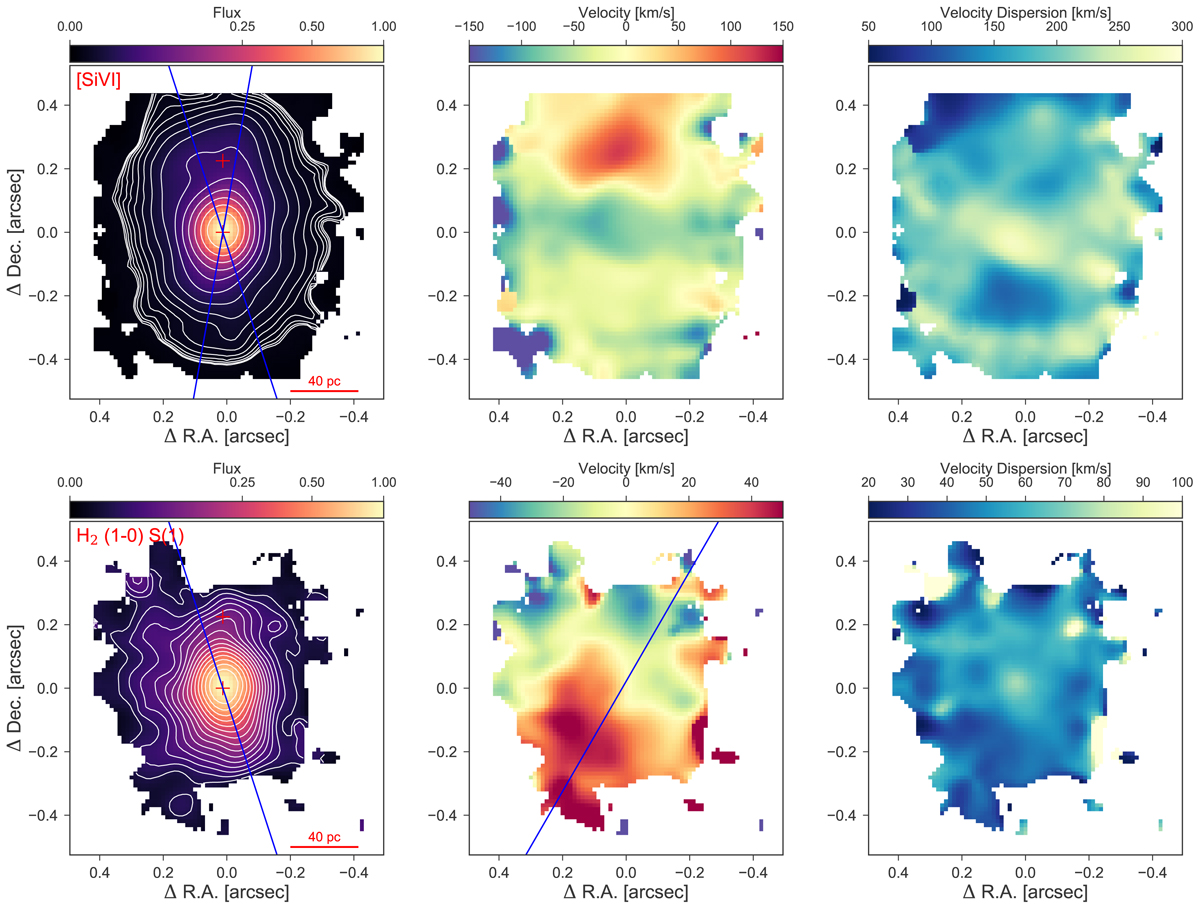
Normalised flux (left), LOS velocity (middle), and velocity dispersion (right) maps of the [Si VI] line (top row) and H₂ (1–0) S(1) line (bottom row). The maps were measured from the same SINFONI cube from which we derived the Brγ profile used in our BLR modelling. The red crosses indicate the locations of the spaxels used to show example line fits in Fig. 17. The blue lines in the [Si VI] flux map show a PA of −18° and +10° which were estimated from the contours of the flux distribution (white contours). The blue line in the H₂ flux map shows a PA of +10° estimated from the contours of the flux distribution (white contours). The blue line in the H₂ velocity map shows a PA of −20° estimated visually from the velocity field.