| Issue |
A&A
Volume 647, March 2021
|
|
|---|---|---|
| Article Number | A49 | |
| Number of page(s) | 16 | |
| Section | Stellar atmospheres | |
| DOI | https://doi.org/10.1051/0004-6361/202040132 | |
| Published online | 09 March 2021 | |
Chemical analysis of early-type stars with planets★
1
Instituto de Ciencias Astronómicas, de la Tierra y del Espacio (ICATE-CONICET), C.C 467,
5400
San Juan, Argentina
e-mail: csaffe@conicet.gov.ar
2
Universidad Nacional de San Juan (UNSJ), Facultad de Ciencias Exactas, Físicas y Naturales (FCEFN), San Juan, Argentina
3
Instituto de Investigación Multidisciplinar en Ciencia y Tecnología, Universidad de La Serena,
Raúl Bitrán 1305,
La Serena, Chile
4
Departamento de Física y Astronomía, Universidad de La Serena,
Av. Cisternas 1200 N,
La Serena, Chile
5
Consejo Nacional de Investigaciones Científicas y Técnicas (CONICET), Argentina
Received:
14
December
2020
Accepted:
11
January
2021
Aims. Our goal is to explore the chemical pattern of early-type stars with planets, searching for a possible signature of planet formation. In particular, we study a likely relation between the λ Boötis chemical pattern and the presence of giant planets.
Methods. We performed a detailed abundance determination in a sample of early-type stars with and without planets via spectral synthesis. Fundamental parameters were initially estimated using Strömgren photometry or literature values and then refined by requiring excitation and ionization balances of Fe lines. We derived chemical abundances for 23 different species by fitting observed spectra with an iterative process. Synthetic spectra were calculated using the program SYNTHE together with local thermodynamic equilibrium ATLAS12 model atmospheres. We used specific opacities calculated for each star, depending on the individual composition and microturbulence velocity vmicro through the opacity sampling method. The complete chemical pattern of the stars were then compared to those of λ Boötis stars and other chemically peculiar stars.
Results. We compared the chemical pattern of the stars in our sample (13 stars with planets and 24 stars without detected planets) with those of λ Boötis and other chemically peculiar stars. We have found four λ Boötis stars in our sample, two of which present planets and circumstellar disks (HR 8799 and HD 169142) and one without planets detected (HD 110058). We have also identified the first λ Boötis star orbited by a brown dwarf (ζ Del). This interesting pair, the λ Boötis star and brown dwarf, could help to test stellar formation scenarios. We found no unique chemical pattern for the group of early-type stars bearing giant planets. However, our results support, in principle, a suggested scenario in which giant planets orbiting pre-main-sequence stars possibly block the dust of the disk and result in a λ Boötis-like pattern. On the other hand, we do not find a λ Boötis pattern in different hot-Jupiter planet host stars, which does not support the idea of possible accretion from the winds of hot-Jupiters, recently proposed in the literature. As a result, other mechanisms should account for the presence of the λ Boötis pattern between main-sequence stars. Finally, we suggest that the formation of planets around λ Boötis stars, such as HR 8799 and HD 169142, is also possible through the core accretion process and not only gravitational instability.
Key words: stars: early-type / stars: abundances / planetary systems
Table A.1 is only available at the CDS via anonymous ftp to cdsarc.u-strasbg.fr (130.79.128.5) or via http://cdsarc.u-strasbg.fr/viz-bin/cat/J/A+A/647/A49
© ESO 2021
1 Introduction
The λ Boötis stars are a group of chemically peculiar objects on the upper main-sequence, showing underabundances (~1–2 dex) of iron-peak elements and near-solar abundances of C, N, O, and S (e.g., Kamp et al. 2001; Heiter 2002; Andrievsky et al. 2002). The class was discovered by Morgan et al. (1943) and named following the bright prototype λ Boötis, which is one extreme member of the class. This group of refractory-poor objects comprises about 2% of early B through early F stars (Gray & Corbally 1998; Paunzen 2001). However, among the pre-main-sequence Herbig Ae/Be stars, that is to say the progenitors of A-type stars, the λ Boötis-like fraction is about 33% (Folsom et al. 2012). The origin of the peculiarity still remains a puzzle, as we can read in the recent discussion of Murphy & Paunzen (2017). Unlike common chemical peculiarities seen in Am and Ap stars, λ Boötis stars are not constrained to slow rotation (Abt & Morrell 1995; Murphy et al. 2015). Cowley et al. (1982) first suggested that λ Boötis could possibly originate from the interstellar medium (ISM) with a nonsolar composition, or from the separation of grains and gas. Then, Venn & Lambert (1990) proposed that λ Boötis stars likely occur when circumstellar gas is separated from grains and then accreted to the stars due to the similarity ofits abundance pattern with the ISM. Other proposed mechanisms include the interaction of a star with a diffuse interstellar cloud (Kamp & Paunzen 2002; Martinez-Galarza et al. 2009), where the underabundances are produced by different amounts of accreted material. Turcotte & Charbonneau (1993) estimated that once the accretion stops, the photospheric mixing and meridional circulation would erase this peculiar signature on a ~1 Myr timescale. By studying thedistribution of λ Boötis stars on the HR diagram, Murphy & Paunzen (2017) conclude that multiple mechanisms could result in a λ Boötis spectra, depending on the age and environment of the star.
In addition to the mentioned scenarios, a number of works propose a possible relation between the λ Boötis phenomena and the presence of planets. For instance, Gray & Corbally (2002) suggested that planetary bodies could perturb the orbits of comets and volatile-rich objects, likely sending them toward the star and possibly originating this pattern. Marois et al. (2008) detected three planets and a debris disk by direct imaging orbiting around the bright A5-type star HR 8799. This object was one of the first early-type stars with planets detected, also showing λ Boötis-like abundances (Gray & Kaye 1999; Sadakane 2006). Then, Kama et al. (2015) studied the chemical abundances and disk properties for a sample of pre-main-sequence Herbig Ae/Be stars. They propose that the depletion of heavy elements observed in ~33% of these stars (Folsom et al. 2012), originates when Jupiter-like planets (with mass between 0.1 and 10 MJup) block the accretion of part of the metal-rich dust of the primordial disk, while gas-phase C and O continues to flow toward the central star. The authors also suggest that main-sequence stars, with a λ Boötis fraction of ~2%, do not host massive protoplanetary disks and then their peculiarity should disappear on a ~1 Myr timescale. Consistent with this picture is also HD 139614, a 13-Myr old pre-main-sequence λ Boötis star (Murphy et al. 2021). For the case of main-sequence stars, Jura (2015) proposed that this peculiar abundance pattern could also be directly originated from the winds of hot-Jupiters, taking the planet as a possible source of gas relatively near to the star. However, he caution that other channels could likely result in the λ Boötis pattern (see e.g., Murphy & Paunzen 2017). Recently, Kunimoto et al. (2018) simulated numerically the pre-main-sequence evolution of stars including the effects of planet formation, and concluded that stars with Teff > 7000 K may show a metallic deficit compatible with the refractory-poor λ Boötis stars. Therefore, the possible link between planet-bearing stars and the λ Boötis chemical pattern motivated the present study.
To date, important trends are known for the case of late-type stars with planets, such as the giant planet-metallicity correlation (Santos et al. 2004, 2005; Fischer & Valenti 2005; Johnson et al. 2010a; Sousa et al. 2011). However, early-type stars with planets are poorly studied compared to late-type stars. This is partly because hot stars rotate rapidly and have few spectral lines, making radial velocity searches of planets more difficult. Transit and microlensing surveys are also more sensitive to planets orbiting low-mass stars (although for different reasons, see e.g., Wright & Gaudi 2013). In the past few years, a slowly growing number of planets orbiting early-type stars were found, detected mainly by transits (e.g., from the KELT Collaboration, Pepper et al. 2007) and also from direct imaging (such as the GPIES survey, Nielsen et al. 2019). This give us the opportunity to start a homogeneous study of this interesting group of stars, by performing (to our knowledge, for the first time) a detailed chemical analysis, allowing a comparison with the λ Boötis pattern. Our sample includes some remarkable objects (such as HR 8799, β Pictoris, Fomalhaut, KELT-9), some important prototype and standard stars for comparison (λ Boötis, Vega), and a number of stars for which no abundance study was previously performed in the literature (HR 4502 A, BU Psc, HD 105850, HD 110058, HD 129926, HD 153053, HD 156751, HD 188228, HD 23281, HD 50445, HD 56537 and V435 Car).
This work is organized as follows. In Sect. 2 we describe the observations and data reduction, while in Sect. 3 we present the stellar parameters and chemical abundance analysis. In Sect. 4 we show the results and discussion, and finally in Sect. 5 we highlight our main conclusions.
2 Stellar samples and observations
We compiled a list of early-type stars with planets taken from the Extrasolar Planets Encyclopaedia1. These stars comprise mainly A-type and few F-type stars, and are listed in the Table 1. Some stars listed in the mentioned catalog present companions with masses above ~13 MJup, the minimum mass to burn Deuterium (e.g., Grossman & Graboske 1973; Saumon et al. 1996). These stars are likely orbited by brown dwarfs (BDs) rather than planets, and some of them are also included in this work for comparison. We also included a group of early-type stars without planets nor brown dwarfs detected, taken from the GPIES imaging survey (Nielsen et al. 2019), which is mainly focused on young and nearby stars. We note that the stars included in this work were taken from different surveys using, for example, transits and imaging, for which the comparisons should be then performed with caution. We also take the opportunity and include in our sample the stars Vega and λ Boötis, as standard or prototype stars for comparison.
Overall, the sample of stars analyzed in this work consists of 37 objects, including 13 stars with planets (detected by transits or direct imaging), 3 stars likely orbited by brown dwarfs and 21 objects without planets nor brown dwarfs detected. The effective temperatures cover 6730 K < Teff < 10 262 K and superficial gravities between 3.60 < log g < 4.37. The complete list of stars analyzed in this work is presented in Table 1, showing the name of the star, spectral type (taken from the SIMBAD2 database), companion detection method (transits, imaging or RV), companion mass, type of companion (planet or brown dwarf), infrared IR excess, source of the spectra, signal-to-noise ratio (S/N) measured at ~5000 Å, and finally the reference for the companion data and/or IR excess. The column labeled IR Excess was added to give information about the possible presence of circumstellar dust orbiting around the stars.
We downloaded archive spectra for the case of HARPS, HARPS-N, HIRES, SOPHIE and ELODIE spectrographs. General characteristics of these instruments are shown in the Table 2, including the resolving power, CCD detector, pixel size, telescope and approximate wavelength range. The reduction was performed by using the Data Reduction Software (DRS) pipeline for the case of HARPS and HARPS-N spectra3, using the reduction package MAKEE 3 with HIRES spectra4, the DRS pipeline with SOPHIE spectra5 and the TACOS program with ELODIE spectra6. The continuum normalization and other operations (such as Doppler correction and combining spectra) were performed using Image Reduction and Analysis Facility (IRAF)7.
We also completed the sample with observations obtained at Complejo Astrónomico El Leoncito (CASLEO) during the observing runs 2018A, 2018B and 2019A. We used the Jorge Sahade 2.15 m telescope equipped with a REOSC high-resolution echelle spectrograph8 and a TEK 1024 × 1024 CCD detector. The REOSC spectrograph uses gratings as cross dispersers, selecting in this case a grating with 400 lines mm−1. We take a number of stellar spectra for each target, followed by a ThAr lamp in order to derive an appropriate pixel versus wavelength solution. The REOSC spectra were reduced using IRAF by performing the usual operations including, for example, bias subtraction, flat fielding, spectral order extraction and wavelength calibration. The final spectra covered the visual range λλ3800–6000, and the average S/N of the spectra was around ~350.
We present in Fig. 1 a theoretical HR diagram (log Teff versus log L∕L⊙) for the stars in our sample. The luminosity L was evaluated from the visual magnitude corrected by interstellar reddening according to the extinction maps of Schlegel et al. (1998)9, following the procedure of Bilir et al. (2008). We used Gaia DR2 parallaxes (Gaia Collaboration 2018) and bolometric corrections interpolated in the tables of Flower et al. (1996). Stars with planets, without planets and with a BD companion are shown with filled circles, empty circles and crosses, respectively. We also show PARSEC evolutionary tracks (Bressan et al. 2012) for stars with different masses. Blue and magenta lines correspond to main-sequence and evolved phases.
Sample of stars studied in this work.
General characteristics of the spectrographs used in this work.
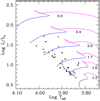 |
Fig. 1 Effective temperature versus luminosity for stars with planets, without planets and with a BD companion (filled circles, empty circles and crosses). Evolutionary tracks for stars of different masses are shown in blue/magenta for main-sequence/evolved stars. The numbers are expressed in solar masses. |
3 Stellar parameters and abundance analysis
3.1 Effective temperature and gravity
Effective temperature Teff and superficial gravity logg were first estimated by using the Strömgren uvbyβ mean photometry of Hauck & Mermilliod (1998) for most stars in our sample or by taking previously published results. We used the program TempLogG (Kaiser 2006) together with the calibration of Napiwotzki et al. (1993) and derredennedcolors according to Domingo & Figueras (1999), in order to derive the fundamental parameters. Then, these values were refined (when neccesary and/or possible) by enforcing excitation and ionization balances of the iron lines. The same strategy was previously applied in the literature (e.g., Acke & Waelkens 2004; Saffe & Levato 2014). The values derived in this way are listed in the Table 3, with an average dispersion of ~175 K and ~0.15 dex for Teff and log g. In the Fig. 2 we compare Teff values with those collected from literature (Erspamer & North 2003; Lepine et al. 2003; Paunzen et al. 2006; Masana et al. 2008; Zorec & Royer 2012; De Rosa et al. 2016; Zhou et al. 2016; Kahraman Alicavus et al. 2016; Gray et al. 2017; Lund et al. 2017; Talens et al. 2017; Borsa et al. 2019), showing a general agreement. Average dispersion bars are shown in the upper left corner of the panel.
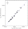 |
Fig. 2 Effective temperature Teff derived in this work versus literature data. Average dispersion bars are shown in the upper left corner of the panel. |
3.2 Rotational velocities v sin i
Projected rotational velocities vsini were first estimated by fitting the observed profile of the line Mg II 4481.23 Å and then refined by fitting most Fe I and Fe II lines inthe spectra. Synthetic spectra were calculated using the program SYNTHE (Kurucz & Avrett 1981) together with ATLAS12 (Kurucz 1993) model atmospheres, and then convolved with a rotational profile (using the Kurucz’s command rotate) and with an instrumental profile for each spectrograph (using the command broaden). Rotational velocities were varied for each line, adopting as final value the average of different lines. The resulting v sin i values are shown in the 4th column of Table 3, covering between 14.8 and 153.5 km s−1 for the stars in our sample. The average dispersion in vsini resulted ~2.2 km s−1. In the Fig. 3 we compare vsini values derived in this work with those from literature, showing a general agreement. Average dispersion bars are shown in the upper left corner of the panel.
3.3 Microturbulence velocity
Microturbulence velocity vmicro is commonlyused as a free parameter in abundance analysis. Several studies have found that microturbulence appears to vary systematically with Teff for early-type stars (Chaffee 1970; Nissen 1981; Coupry & Burkhart 1992; Gray et al. 2001; Takeda et al. 2008; Gebran et al. 2014). They showed that vmicro increases with increasing Teff, peaking around mid-A type (~8500 K), before falling away to almost ~0 km s−1 for B-type stars. In this work, we adopted the formula derived by Gebran et al. (2014) in order to estimate vmicro as a function of Teff, which is valid for ~6000 K < Teff < ~10 000 K. Gebran et al. (2014) showed that the formula has an uncertainty of ~25%, which we adopted as the error in the vmicro values. The effect of this relatively large uncertainty (and uncertainties of other fundamental parameters) on the abundance values is estimated in the next sections.
Fundamental parameters derived for the stars in this work.
3.4 Abundance analyses
We applied an iterative procedure to determine the chemical abundances for the stars in our sample. We started by computing an ATLAS12 (Kurucz 1993) model atmosphere for the adopted Teff, log g and vmicro values. For this initial model, we used solar metallicity values taken from Asplund et al. (2009). The abundances were determined by fitting a synthetic spectra to the different lines using the program SYNTHE (Kurucz 1993). With the new abundance values, we derived a new model atmosphere and started the process again. If neccessary, Teff and log g were refined to achieve the balance of Fe I and Fe II lines. In each step, opacities were calculated for an arbitrary composition and vmicro using the opacity sampling (OS) method, similar to previous works (Saffe et al. 2018, 2019, 2020). In this case, two runs of ATLAS12 are used (see e.g., Castelli 2005; Saffe et al. 2018): the first for a preselection of important lines and the second for the final calculation of the model structure. In this way, abundances are consistently derived using specific opacities rather than solar-scaled values. An estimation of the differences obtained when using these two approaches for the case of solar-type stars, can be seen in Saffe et al. (2018).
We compared observed and synthetic spectra using a χ2 function, calculated as the quadratic sum of the differences between both spectra. The abundances were varied in steps of 0.01 dex until reach a minimum in χ2, similar to Saffe & Levato (2014). The fits were also verified by eye inspection, using intervals spanning 10 Å around the lines of interest. Abundances derived in this way are presented in the Table A.1, showing the average and dispersion for the stars in our sample. The values are shown using the square bracket notation, which denotes abundances relative to the Sun, that is to say [N/H] = log(N/H)Star − log(N/H)Sun, where log(N/H)Star and log(N/H)Sun are abundance values for the star and for the Sun, the later taken from Asplund et al. (2009).
Chemical abundances were derived for 23 different species, including C I, C II, O I, Mg I, Mg II, Al I, Al II, Si II, Ca I, Ca II, Sc II, Ti II, Cr II, Mn I, Mn II, Fe I, Fe II, Ni II, Zn I, Sr II, Y II, Zr II and Ba II. The atomic line list and laboratory data used in this work are basically those described in Castelli & Hubrig (2004), updated with specialized references as described in Sect. 7 of González et al. (2014). In Figs. 4 to 6 we present an example of observed, synthetic, and difference spectra (black, blue dotted, and red lines) for the stars in our sample. The stars are sorted in the plot by increasing v sin i. There is a good agreement between modeling and observations for the lines of different chemical species.
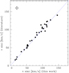 |
Fig. 3 Projected rotational velocity vsini derived in this work versus literature data. Average dispersion bars are shown in the upper left corner of the panel. |
3.5 Uncertainty of abundance values
In general, the uncertainty in the abundance values have different sources. First, we estimated the measurement error e1 from the line-to-line dispersion as  , where σ is the standard deviation of the line-by-line abundances and n is the number of lines. For elements with only one line, we adopted for σ the standard deviation of the iron lines. Then, we determined the contribution to the abundance error due to the uncertainty in stellar parameters. We modified Teff and logg by their uncertainties and recalculated the abundances, obtaining the corresponding differences e2 and e3. We also wanted to estimate the contribution to the error due to the uncertainty in vmicro, which is not always included in the error calculation. Similarly, we modified vmicro by its uncertainty and obtained thedifference e4 by recalculating the abundances. Finally, the total error was estimated as the quadratic sum of e1, e2, e3 and e4. These values are presented in the Table A.1, in order to determine their contribution to the total error.
3.6 NLTE effects
The basic difference between local thermodynamic equilibrium (LTE) and NLTE is the behavior of atomic level populations. LTE allows a relatively simple calculation using a Saha-Boltzman distribution, while in NLTE the level populations are affected by the radiation field and should be determined by kinetic equilibrium (see e.g., Kubát 2014). Departures from LTE are more pronounced in stars with high temperature and with low gravity and metallicity. For instance, the reduction of surface gravity results in a decreased efficiency of collisions with electrons and hydrogen atoms, reducing the thermalizing effect, which leads to stronger NLTE effects (e.g., Gratton et al. 1999). Subsequently, some particular species and transitions should be taken with caution.
Rentzsch-Holm (1996) estimated NLTE departures for C I lines in early-type stars (up to ~0.2 dex for lines with equivalent widths Weq ~ 100 mÅ, and lower departures with decreasing Weq). Weak and intense C II lines could also show pronounced NLTE effects (Przybilla et al. 2011), except for C II 5145 Å and other members of the multiplet. For O I, NLTE effects are expected, especially in the near-IR triplet O I 7771 Å and the other lines of the same multiplet (e.g., Sitnova et al. 2013; Przybilla et al. 2011). For the case of Mg, Przybilla et al. (2001) found that the intense line Mg II 4481 systematically yields notably higher abundances due to NLTE effects (between 0.2 and 0.8 dex for early-type stars). More recently, Alexeeva et al. (2018) studied the formation of Mg lines under LTE and NLTE. For stars with 7000 K < Teff < 17 500 K, they recommend to use the Mg II lines 3848.21, 4427.99, 4384.64 and 4390.57 Å even at the LTE assumption. However, these lines are not always available in our spectra. For stars with 7000 K < Teff < 8000 K, they showed that the line 4702.99 and the Mg I b triplet could be safely used in LTE. For each star, they also estimate that the average difference between Mg I and Mg II diminish from ~0.23 dex in LTE to ~0.09 dex in NLTE. This could explain, at least in part, the higher abundances of Mg II compared to Mg I observed in some stars. However, the authors also caution that the difference Mg II − Mg I even in NLTE could amount up to ~0.24 dex for metal-poor stars, for a reason that require future investigation. For the case of Ti II, Sitnova et al. (2016) showed some small NLTE departures (for instance, up to ~0.03 dex for the line 5336.79) and originating possible discrepancies between Ti I and Ti II.
3.7 Comparison with literature
We present in Fig. 7 a comparison of metallicity values derived in this work and from literature. We collected these values from different sources (Andrievsky et al. 2002; Erspamer & North 2003; Gray et al. 2006; Sadakane 2006; Collier Cameron et al. 2010; Yoon et al. 2010; Prugniel et al. 2011; Folsom et al. 2012; Moór et al. 2013; Bieryla et al. 2014; Zhou et al. 2016; Gaudi et al. 2017; Luck 2017; Lund et al. 2017; Talens et al. 2017; Temple et al. 2017; Anderson et al. 2018; Bochanski et al. 2018; Arentsen et al. 2019; Cheng et al. 2019). The Fig. 7 shows a good agreement with literature data in general for most stars. The point in the lower corner of the plot corresponds to the star λ Boötis.
The largest differences in metallicity correspond to the stars KELT-17 and HD 88955, with [Fe/H] differences of 0.48 and 0.56 dex, respectively. Both stars are identified in Fig. 7. Given the relatively large differences, we briefly explore the possible source of the discrepancies. Zhou et al. (2016) discovered a giant planet around KELT-17 and adopted a final [Fe/H] value of −0.018 ± 0.073 dex by iterating through a global analysis of the transit, constrained by a transit-derived stellar density and stellar isochrone models. The authors also note that, when using only spectroscopic data (a single interval centered around the Mg b lines), the resulting metallicity could vary between −0.10 ± 0.08 dex and +0.25 ± 0.08 dex (by fixing the logg value). In this way, the global solution adopted by Zhou et al. (2016) depends on several parameters and models, not specifically designed to derive abundances. On the other hand, Saffe et al. (2020) show that the chemical pattern of KELT-17 closely resembles those of Am stars (for many species and not only iron), using a process different than those used by Zhou et al. (2016).
The other star with a notable difference in metallicity is HD 88955. Erspamer & North (2003) derived [Fe/H] = 0.06 dex for this object using an automatic procedure with ELODIE (R ~ 42 000) spectra. They used a spectral synthesis program (modified by the authors) in order to accept ATLAS9 model atmospheresinstead of ATLAS5 models as in their original version. On the other hand, for this star we obtained [Fe/H] = −0.50 ± 0.14 dex using HARPS (R ~ 115 000) spectra together with ATLAS12 models. The difference is possibly due to the adopted stellar parameters (difference of 220 K in Teff and 0.37 dex in logg) and laboratory data for the lines. Unfortunately, Erspamer & North (2003) do not report a [Fe/H] error for this star, which makes a later comparison more complicated.
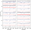 |
Fig. 4 Observed, synthetic, and difference spectra (black, blue dotted, and red lines) for the stars in our sample, sorted by v sin i. |
4 Discussion
In the present section, we discuss different aspects related to the metallic content of the early-type stars with planets. We start by searching λ Boötis stars in our sample and studying the possible relation between hot-Jupiter planets and λ Boötis stars. Then, we search for other possible chemically peculiar stars in our sample. Finally, we discuss the possible implicationsof our results within the context of the planet formation models.
4.1 λ Boötis stars in our sample
We compared the abundances of our sample stars with the average pattern of λ Boötis stars. As explained in the Introduction, λ Boötis stars are early-type objects showing underabundances (~1–2 dex) of iron-peak elements and near-solar abundances of C, N, O and S (e.g., Kamp et al. 2001; Heiter 2002; Gray et al. 2017). A representative chemical pattern was derived by using the average of 12 λ Boötis stars taken from Heiter (2002). As result of this comparison, we have identified four (or five) stars with the λ Boötis pattern: HD 110058, HD 169142, HR 8799 and ζ Del (the star λ Boötis itself would be the 5th object). We present in the Fig. 8 the abundances of these four stars, compared to the average pattern of λ Boötis stars. The vertical barsin the average λ Boötis pattern correspond to the standard deviation of the different stars, as derived by Heiter (2002). The figure shows two panels for each star, corresponding to elements with atomic number z < 32 and z > 32. In general, these stars present near-solar values of C and O, together with subsolar values of the other metals. An individual description for each star can be read in the Appendix B. HD 169142 was also previously identified as a λ Boötis object (Folsom et al. 2012; Gray et al. 2017), as well as HR 8799 (Gray & Kaye 1999; Sadakane 2006) and λ Boötis (Venn & Lambert 1990; Paunzen et al. 1999; Cheng et al. 2019).
Most of the λ Boötis stars identified here present evidence of circumstellar material. HR 8799 and HD 169142 are orbited by dusty disks and planets detected by direct imaging (Marois et al. 2008; Fedele et al. 2017). Up to now, there is no planet detected around HD 110058, although presents an IR excess indicative of a dusty disk (Nielsen et al. 2019; Esposito et al. 2020). It is also interesting to note that ζ Del is orbited by a brown dwarf detected by direct imaging (De Rosa et al. 2014), with a projected separation of 13.51 ± 0.08 arcsec, or 912 ± 5 AU at the distance of ζ Del. There is also evidence of IR excess around ζ Del likely related to the presence of dust (Nielsen et al. 2019; Esposito et al. 2020). To our knowledge, ζ Del is the first λ Boötis star orbited by a brown dwarf, which could be used as a laboratory to test stellar formation scenarios. Interestingly, our sample includes other two stars orbited by brown dwarfs (59 Dra and β Cir), although not showing λ Boötis characteristics.
We also present in the Fig. 9 the abundances of HD 156751, which shows a less clear λ Boötis signature (their ~solar values of Sr, Y and Ba are not typical of λ Boötis stars). The same Fig. 9 presents the star λ Boötis itself, which shows rather extreme characteristics for its class (a very low metallic content). Up to now, there is no planet detected around HD 156751 nor λ Boötis (Nielsen et al. 2019), while there is IR excess detected around λ Boötis indicative of a dusty disk (Rieke et al. 2005; Su et al. 2006).
In our sample of early-type stars, there is no obvious relation between the presence of planets (13 stars) and the λ Boötis pattern (4 objects, or 5 if we include the star λ Boötis). Kama et al. (2015) proposed that the λ Boötis observed in ~33% of pre-main-sequence Herbig AeBe stars (Folsom et al. 2012), originates when Jupiter-like planets (with mass between 0.1 and 10 MJup) block the accretion of dust from the primordial disk. Our sample includes the star HD 169142, which have been classified as a young pre-main-sequence object and also as a λ Boötis star(Folsom et al. 2012). This object is included in our sample and shows the mentioned chemical peculiarity (see Fig. 8). Although not strictly a pre-main-sequence object, HR 8799 is also a young star (age of 42 ± 5 Myr, Nielsen et al. 2019) which shows the λ Boötis signature (see Fig. 8). Then, the λ Boötis signature that we observe in these two stars, support in principle the scenario proposed by Kama et al. (2015).
It is worthwhile mentioning that β Pictoris and HD 95086 are also young stars (ages <~50 Myr) hosting giant planets (Lagrange et al. 2019; De Rosa et al. 2016), but not showing a clear λ Boötis signature. β Pictoris is sligthly metal-poor (including C), while Ca and Ba show solar values. Its λ Boötis classification was initially suggested based on its evolutionary status and the presence of a circumstellar disk (King & Patten 1992). However, this peculiar classification was then ruled out by different authors, using an optical spectral (Holweger et al. 1997)and also from the ratio of UV lines (Cheng et al. 2016). In this work, we do not identify the star β Pictoris with a λ Boötis pattern. The other young star (HD 95086) presents mostly solar or very slightly subsolar abundances, different than average λ Boötis stars. However, the fact that these young stars (β Pictoris and HD 95086) do not display the λ Boötis peculiarity, do not rule out the scenario proposed by Kama et al. (2015). β Pictoris and HD 95086 are young stars although not strictly accreting pre-main-sequence objects. Kama et al. (2015) propose that for main-sequence stars without a massive protoplanetary disk (that is, after the accretion of volatile-rich gas), the peculiarity should disappear on a short timescale (~1 Myr), as estimated by Turcotte & Charbonneau (1993). Following the scenario of Kama et al. (2015), it is possible that these young stars showed the λ Boötis peculiarity in the past, which was then erased few Myrs ago.
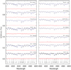 |
Fig. 5 Observed, synthetic, and difference spectra (black, blue dotted, and red lines) for the stars in our sample, sorted by v sin i. |
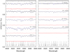 |
Fig. 6 Observed, synthetic, and difference spectra (black, blue dotted, and red lines) for the stars in our sample, sorted by v sin i. |
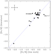 |
Fig. 7 Metallicity values derived in this work ([Fe/H]) versus literature data. Average dispersion bars are shown in the upper left corner of the panel. The stars HD 88955 and KELT-17 are identified in the plot (see text for more details). |
4.2 λ Boötis stars and hot-Jupiter planets
Hot-Jupiter planets present short orbital periods (<10 d) and large planetary masses (>0.1 MJup), that is, theyare gas giants orbiting very close to their stars (e.g., Wang et al. 2015). Recently, Jura (2015) proposed that λ Boötis stars could be originated by accreting volatile-rich gas from the winds of hot-Jupiter planets, rather than from the interaction with a molecular cloud. In our sample, there are some stars orbited by hot-Jupiter planets, all detected by the transits technique: WASP-33, WASP-167, WASP-189, KELT-9, KELT-17, KELT-20, MASCARA-1 and HAT-P-49. We present in the Figs. C.1 and C.2, the abundances of these hot-Jupiter hosts, compared to the average pattern of λ Boötis stars. We do not recognize a clear λ Boötis pattern in these objects. Most of them show approximately solar abundances; the possible exceptions are WASP-167 showing a metal-rich spectra, and KELT-17 which is an Am star (Saffe et al. 2020). KELT-20 presents subsolar metallic abundances, being likely closer to theλ Boötis pattern. However, this star still presents differences with this class ([C/H] = −0.42 ± 0.11 is subsolar, while Si and Ba present suprasolar values), which rule out its λ Boötis nature.
In principle, the abundances derived for these stars do not support the accretion scenario from the winds of hot-Jupiters. This is possibly due to a number of reasons, as explained by Jura (2015). For example, the hot-Jupiter composition is assumed to be nearly solar;the elements in the flow should be efficiently separated (this depends on the viscosity of the gas); the amount of planetary gas expelled (and then accreted onto the star) should be enough to produce the effect; and finally, the flow from the planet should not be magnetically funneled (this perhaps avoid elemental separations). If these conditions are not met, the λ Boötis pattern will likely not appear (Jura 2015). The author caution that other channels could also result in a λ Boötis pattern. In particular, Murphy & Paunzen (2017) conclude that multiple mechanisms could possibly produce a λ Boötis spectra, depending on the age and environment of the star.
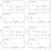 |
Fig. 8 Abundances of four early-type stars (black), compared to the average pattern of λ Boötis stars (blue). We show two panels for each star, corresponding to elements with z < 32 and z > 32. |
4.3 Other chemically peculiar stars in our sample
We also compared the abundances of the early-type stars with those of chemically peculiar Am, ApSi and HgMn stars. In this case, the origin of their peculiar abundances is commonly attributed to diffussion processes (e.g., Michaud 1970; Michaud et al. 1976, 1983; Vauclair et al. 1978; Richer et al. 2000), taking place in the stable atmospheres of slowly rotating A-type stars. In principle, there is no direct relation between these peculiar patterns and the presence of planets. After inspecting the chemical patterns of our early-type stars, we only found one clear Am object: the exoplanet host star KELT-17 (Saffe et al. 2020). In general, Am stars present overabundances of most heavy elements in their spectra, particularly Fe and Ni, together with underabundances of Ca II and Sc II (see e.g., the work of Catanzaro et al. 2019, and references therein). We compared the abundances of KELT-17 with an average pattern of 62 Am stars recently determined by Catanzaro et al. (2019) and found a good agreement, as we can see in the Fig. 10. KELT-17 is the first exoplanet host whose chemical pattern was identified as an Am star (Saffe et al. 2020), being an early result of this study. Although not included in the present sample, other planet bearing stars with a possible Am pattern include KELT-19 (Siverd et al. 2017) and KELT-26 A (Rodríguez Martínez et al. 2019).
In general, by inspecting the abundances of the planet host stars in our sample, we found a number of stars showing mostly solar values (Fomalhaut, KELT-9, MASCARA-1, WASP-33, HAT-P-49 and WASP-189). Other objects show a λ Boötis signature (such as the young stars HD 169142 and HR 8799), while other planet hosts show a subsolar or slightly subsolar metallic content (β Pictoris, HD 95086 and KELT-20). In addition, we also found a chemically peculiar Am star (KELT-17) and a metal-rich star (WASP-167). Then, no single chemical pattern could account for the complete group of planet bearing stars.
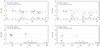 |
Fig. 9 Abundances of the stars HD 156751 and λ Boötis (black), compared to the average pattern of λ Boötis stars (blue). We show two panels for each star, corresponding to elements with z < 32 and z > 32. |
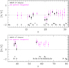 |
Fig. 10 Abundances of the exoplanet host star KELT-17 (black), compared to the average pattern of Am stars (magenta). The two panels correspond to elements with z < 32 and z > 32. |
4.4 Early-type stars and models of planet formation
In this section we briefly review planet formation models and the possible relation to our observations. The two main models of planet formation are the Core Accretion (CA) and the Gravitational Instability (GI). In the CA model, the accretion of dust particles and planetesimals could result in a solid core of few M⊕, forming low-mass planets and cores of giant planets. If the core reach a critical mass of ~5–10 M⊕ before the dissipation of gas disk, then they could undergo a runaway accretion of gas and form giant planets (e.g., Safronov & Zvjagina 1969; Pollack et al. 1996; Ida & Lin 2004; Alibert et al. 2005, 2011; Mordasini et al. 2012). In the GI model, amassive and cold protoplanetary disk fragments into clumps which then cool and contract to form giant planets (e.g., Kuiper 1951; Boss 1998, 2002, 2017). In the last years, CA models become the dominant planet formation theory for solar-mass stars, matching observed features such as the abundance of Neptune and Jupiter-mass planets (e.g., Udry et al. 2007) and the planet-metallicity correlation (Ida & Lin 2004; Mordasini et al. 2012). On the other hand, initial GI models cannot provide an explanation of the planet-metallicity correlation10. Both CA and GI models have received considerable improvements in the last years (such as planet migration, peeble accretion, etc.) and are still under developement (see e.g., the reviews of Lissauer & Stevenson 2007; Durisen et al. 2007; Helled et al. 2014; Raymond & Morbidelli 2020).
It has been claimed that, for solar-type stars, CA models could face some difficulties (in principle) explaining the presence of giant planets around metal-poor stars, or massive planets at long radial distances (see e.g., Helled et al. 2014). In particular, HR 8799 is a metal-poor A5 star included in our sample, hosting three giant planets orbiting beyond 10 AU (Marois et al. 2008). Then, some authors proposed that the planets orbiting HR 8799 are likely formed by GI, given that GI models can take place at large radii and in low metal environments (Marois et al. 2008; Dodson-Robinson et al. 2009; Meru & Bate 2010). Other works cast some doubts about the planet formation around HR 8799, showing that CA models are also possible (Currie et al. 2011) or even a combination of GI and CA (Marois et al. 2010). For the case of β Pictoris and HD 169142, also having giant planets at long distances, CA models seem to be favored (GRAVITY Collaboration 2020; Nowak et al. 2020; Pérez et al. 2019). However, an important word of caution about these works is in order. Some of the stars mentioned (HR 8799 and HD 169142) display (superficial) metal-poor abundances, showing in fact a λ Boötis pattern (see for example Fig. 8). As previously mentioned, the most accepted idea about the origin of this peculiar signature, suppose a solar-like composition for the original molecular cloud where the stars born, and then some kind of selective accretion to obtain a λ Boötis pattern. In this way, it would be not entirely appropriate to assume a metal-poor natal environment for stars like HR 8799, as assumed by some works to support a GI planet formation (e.g., Meru & Bate 2010). This fact was early noted by Paunzen et al. (2014), in their comparison of λ Boötis stars and Population II type stars. Numerical simulations of planet formation around λ Boötis stars should assume a solar-like composition (rather than a metal-poor natal environment), and this could have important consequences for the subsequent results.
We prefer to be more cautious about the origin of planets orbiting around HR 8799 and similar stars, and explore subsequent predictions of CA models, even including a low metallicity natal environment. Alibert et al. (2011) studied the formation of planets under the CA assumption, specially for the case of stars with different masses (0.5, 1.0 and 2.0 M⊙). They found that the metallicity effect of planet formation is weakly dependent on stellar mass, that is, stars hosting giant planets resulted, on average, more metal rich than stars without planets. However, they showed that the metallicity effect depends also on the mass of the disk. If the disk mass scales with the stellar mass, the effect of metallicity decreases as the mass of the primary increases. Then, the minimum metallicity required to form a massive planet is correspondingly lower for massive stars than lower mass stars. Mordasini et al. (2012) also suggest a “compensation effect”, where giant planet cores could form even at low metallicities and large distances but compensated by high disk masses. They caution, however, that low metallicities cannot be compensated by high gas masses ad infinitum, at least if higher mass disks have an ice line farther out due to stronger viscous dissipation. In other words, it seems possible for stars having massive gas disks to form giant planets though CA, without the necessity of higher metallicities.
5 Conclusions
In the present work, we performed a detailed abundance determination for a number of early-type stars with and without planets, by fitting high-resolution stellar spectra with a synthetic spectra. We compared the complete chemical pattern of the sample with those of λ Boötis as well as with other chemically peculiar stars. Then, the main results of this study are as follows:
We have found four λ Boötis stars in our sample, two of which present planets (HR 8799 and HD 169142), one without planets (HD 110058), and the first λ Boötis star orbited by a brown dwarf(ζ Del). This last interesting pair composed by a λ Boötis star+ brown dwarf, could help to test stellar formation scenarios.
We find no unique chemical pattern for (early-type) planet-bearing stars. Within this group, we found λ Boötis stars (HD 8799 and HD 169142), a chemically peculiar Am star (KELT-17), a number of stars showing mostly solar abundaces, and one metal-rich object (WASP-167).
The λ Boötis signature that we observe in the Herbig AeBe star HD 169142 and in the young star HR 8799, support in principle the scenarioproposed by Kama et al. (2015). They suggest that the presence of giant planets in very young stars possibly block the dust from protostellar disks and allow the accretion of volatile-rich gas, resulting in a λ Boötis pattern.
The abundances derived in this work for different hot-Jupiter exoplanet host stars do not support, in principle, the accretion from hot-Jupiters winds proposed to explain the origin of λ Boötis stars. We suggest that other mechanisms should account for the presence of main-sequence λ Boötis stars.
It was previously suggested that gravitational instability could account for the formation of planets around low metallicity stars like HR 8799. However, we caution that it seems also possible for stars having massive gas disks to form giant planets though core accretion.
The interesting initial findings that we found here encourage us to continue investigating early-type stars and the possible relation between planets and λ Boötis stars. We suggest to increase the number of stars studied in order to improve the statistical significance of the results.
Acknowledgements
We thank the referee Dr. Ernst Paunzen for constructive comments that improved the paper. CS acknowledge the project grants CICITCA E1134 and PICT 2017-2294. The authors wish to recognize and acknowledge the very significant cultural role and reverence that the summit of Mauna Kea has always had within the indigenous Hawaiian community. We are most fortunate to have the opportunity to conduct observations from this mountain. The authors also thank Dr. Robert Kurucz for making their codes available to us.
Appendix A Detailed chemical abundances
We present in this section individual abundances for each star, showing average ± total error and the uncertainties e1, …, e4 for the chemical species (see Table A.1).
Appendix B Comments about individual stars
In this section we briefly comment the chemical features that we observe on individual stars.
59 Dra: This object presents mostly solar values. β Cir: This star presents some slightly subsolar abundances (such as [Fe/H] = –0.25 ± 0.26 dex) but also suprasolar values of s-process elements (Sr, Y, Zr and Ba by ~+0.3 dex). In particular, C is clearly subsolar (–0.49 ± 0.17 dex). We do not identify a λ Boötis pattern.
β Pic: This star presents some sligthly subsolar values of some species (for example [Fe/H] = −0.28 ± 0.14 dex) but also solar values of Mg, Ca, Sc, Ti, Y and Ba. C resulted slightly subsolar (−0.20 ~ 0.11 dex). Then, we do not detect clear λ Boötis signature. Its λ Boötis classification was initially suggested based on its evolutionary status and the presence of a circumstellar disk (King & Patten 1992). However, itsλ Boötis nature was then ruled out by using optical spectra (Holweger et al. 1997) and also using the ratio of UV lines (Cheng et al. 2016).
BU Psc:this star resulted sligthly subsolar in some elements (Al, Cr, Fe) although solar in other species (Si, Sc, Ti, Y, Ba).
Fomalhaut: this star shows mostly solar values (such as [Fe/H] = 0.12 ± 0.19 dex), and slightly enriched in Ni and s-process elements (Sr, Y, Zr and Ba). We do not observe λ Boötis-like characteristics.
HD 29391: most metals in this star show solar abundances.
HD 105850: this object shows some slightly depleted elements (Cr, Fe) and some solar species (Ca, Sc, Ti, Zr, Ba). We do not identify a λ Boötis pattern.
HD 110058: we observe a clear λ Boötis pattern. Most metals show very low abundances (between 1 and 2 dex), while C is almost solar ([C/H] = −0.14 ± 0.06 dex), in agreement with most λ Boötis stars.
HD 115820: most elements in this object show solar abundances.
HD 120326: mostly solar values. Some elements are very slightly subsolar (Mn, Fe) while other show solar values (Ca, Sc, Ti, Cr).
HD 129926: Corbally (1984) classified this star as a close binary (F0 V + G1 V), with V magnitudes of 5.10 and 7.12 and a separation of ~8.2 arcsec. He reported strong Sr and Fe II for the primary, and strong lines for the secondary. The HARPS data present a metal-rich spectra, showing similarities but also differences to Am and ApSi stars. For instance, Cr, Fe, and Sr show lower values than ApSi stars, while Ca and Sc show higher values than Am stars.
HD 133803: this star shows solar (or slightly suprasolar) abundances in most elements.
HD 146624: this star presents solar abundances (for example Mg, Si, Ti, Fe). C and O both shows subsolar values.
HD 153053: some species present slightly subsolar values (such as [Fe/H] = −0.29 ± 0.14 dex), while s-process elements show slightly suprasolar abundances (Sr, Y, Zr and Ba by ~+0.3 dex).
HD 156751: this star would classify as mild-λ Boötis, if we only inspect those elements with atomic number z < 28, showing subsolar values of metals (for example [Fe/H] = −0.47 ± 0.17 dex) and near-solar C (−0.13 ± 0.08 dex). However, we also measured solar values for some s-process elements (Sr, Y and Ba), being somewhat higher than average λ Boötis stars.
HD 159492: this object presents mostly solar abundances (such as Mg, Si, Sc, Ti, Cr, Fe).
HD 169142: this star presents a clear λ Boötis pattern. Subsolar abundances of most metals (between 0.50 and 0.75 dex) together with a solar abundance of C ([C/H] = 0.13 ± 0.09 dex). This star was previously identified as a λ Boötis object (Folsom et al. 2012; Gray et al. 2017), although for some authors their λ Boötis pattern is less clear (Murphy et al. 2015). Interestingly, Gray et al. (2017) suggest a likely spectral variation for this star, proposing a follow up to see if its λ Boötis nature could also vary.
HD 188228: mostly solar values (Mg, Si, Ti, Cr, Fe), with subsolar C and suprasolar Ba.
HD 23281: mostly solar values (Mg, Si, Ti, Fe), with slightly subsolar C and suprasolar values of s-process elements (Sr, Y, Zr and Ba).
HD 50445: this star presents some subsolar abundances ([Fe/H] = −0.31 ± 0.13 dex). However, it also shows solar values of Mg, Sr, Y, Zr and Ba unlike most λ Boötis stars.
HD 56537: This object shows some subsolar values (for example [Fe/H] = −0.51 ± 0.13 dex). However, C also shows a low value ([C/H] = −0.42 ± 0.13 dex)), while Ca, Ti, Y and Ba show almost solar values, different of most λ Boötis stars.
HD 88955: this star presents some subsolar abundances (such as [Fe/H] = −0.50 ± 0.14 dex) but also a low value for C (−0.61 ± 0.11 dex). However some s-process species show solar values (Y, Zr, Ba). Then, is different of most λ Boötis stars.
HD 95086: this object presents solar values of most metals.
HR 4502 A: this star presents mostly solar abundances.
HR 8799: this star presents a λ Boötis pattern. Subsolar metallic abundances (between 0.50 and 0.75 dex) together with a near-solar C ([C/H] = −0.11 ± 0.07 dex). Its λ Boötis nature was also previously reported in the literature (Gray & Kaye 1999; Sadakane 2006; Wang et al. 2020).
KELT-17: this object shows a chemically peculiar Am pattern. KELT-17 presents subsolar values of Ca and Sc, while other metals showoverabundances (Ti, Cr, Mn, Fe, Sr, Y, Ba). The Am nature of this star was recently reported by Saffe et al. (2020).
KELT-20: this star presents mostly subsolar values (for example [Fe/H] = −0.35 ± 0.15 dex). However, it also shows a low C abundance ([C/H] = −0.42 ± 0.10 dex), also solar or suprasolar values of Si, Ni and Ba, different of average λ Boötis stars.
KELT-9: this star presents solar abundances for most metals, with slightly subsolar values for Al and Sr.
MASCARA-1: this object shows mostly solar values in general, with suprasolar abundances of Sr, Y, Zr and Ba.
V435 Car: this star presents solar values of most elements.
WASP-33: this star shows mostly solar abundances, together with a suprasolar O abundance. We caution however that, for this star, the O abundance was derived using the O I near-IR triplet at ~7771 Å, which suffer of NLTE effects (e.g., Sitnova et al. 2013; Przybilla et al. 2011). In this star, some s-process elements (Sr, Y and Ba) also show suprasolar values.
HAT-P-49: this object presents mostly solar values, with slightly suprasolar abundances of Sc, Sr and Ba.
λ Boötis: this object is more metal-poor than the average pattern of λ Boötis stars. In addition, this star shows C and O slightly subsolar rather than solar, in agreement with previous works (Venn & Lambert 1990; Paunzen et al. 1999; Cheng et al. 2019). Then, we would consider this object as a rather extreme case of the λ Boötis class.
Vega: this star presents subsolar abundances of most metals and slightly subsolar values of O (−0.36 ± 0.10 dex): these features are, in principle, similar to other λ Boötis stars. However, C presents a lower abundance ([C/H] = −0.33 ± 0.11 dex) than most λ Boötis stars. A λ Boötis nature for this star was previously suggested (Yoon et al. 2010), however this class was then ruled out by Cheng et al. (2016), in agreement with the present work.
WASP-167: this star presents a slightly metal-rich abundance pattern. However, it is different of Am stars (showing higher Ca, Sc and lower Cr, Sr, Y, Zr, Ba), different of ApSi stars (showing lower Ti, Cr, Mn, Fe) and different of HgMn stars (lower Mn and no Hg observed).
WASP-189: this object is listed in the catalog of Renson & Manfroid (2009) of chemically peculiar stars with a “doubtful” A4m classification. Its suspected Am class was then ruled out (Anderson et al. 2018). This star presents Ca and Sc almost solar (different of Am stars), mostly solar abundances and some suprasolar s-process elements (Sr, Y, Zr and Ba), as we can see in the Fig. C.1.
ζ Del: this star shows a clear λ Boötis pattern: subsolar metallic abundances (for example [Fe/H] = −0.68 ± 0.12 dex), together with solar values of both [C/H] and [O/H] (−0.06 ± 0.07 and 0.08 ± 0.13 dex).
Appendix C Abundance pattern of hot-Jupiter stars
We present in this section a number of figures, comparing the abundances of early-type stars which host hot-Jupiter planets, with the chemical pattern of λ Boötis stars.
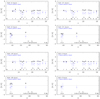 |
Fig. C.1 Abundances of hot-Jupiter host stars (WASP-33, WASP-167, WASP-189 and KELT-9, in black) compared to an average λ Boötis pattern (blue). We show two panels for each star, corresponding to elements with z < 32 and z > 32. See text for more details. |
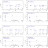 |
Fig. C.2 Abundances of hot-Jupiter host stars (KELT-17, KELT-20, MASCARA-1 and HAT-P-49, in black) compared to an average λ Boötis pattern (blue). We show two panels for each star, corresponding to elements with z < 32 and z > 32. See text for more details. |
References
- Abt, H., & Morrell, N. 1995, ApJS, 99, 135 [Google Scholar]
- Acke, B., & Waelkens, C. 2004, A&A 427, 1009 [NASA ADS] [CrossRef] [EDP Sciences] [Google Scholar]
- Aihara, H., Allende Prieto, C., An, D., et al. 2011, ApJS, 193, 29 [Google Scholar]
- Alexeeva, S., Ryabchikova, T., Mashonkina. L., & Shaoming, H. 2018, ApJ, 866, 153 [Google Scholar]
- Alibert, Y., Mordasini, C., Benz, W., & Winisdoerffer, C. 2005, A&A, 434, 343 [NASA ADS] [CrossRef] [EDP Sciences] [Google Scholar]
- Alibert, Y., Mordasini, C., & Benz, W. 2011, A&A, 526, A63 [NASA ADS] [CrossRef] [EDP Sciences] [Google Scholar]
- Aller, K., Kraus, A., Liu, M., Burgett, W., et al. 2013, ApJ, 773, 63 [Google Scholar]
- Anderson, D., Temple, L., Nielsen, L., et al. 2018, MNRAS, submitted [arXiv:1809.04897] [Google Scholar]
- Andrievsky, S., Chernyshova, I., Paunzen, E., et al. 2002, A&A, 396, 641 [NASA ADS] [CrossRef] [EDP Sciences] [Google Scholar]
- Arentsen, A., Prugniel, P., Gonneau, A., et al. 2019, A&A, 627, 138 [Google Scholar]
- Asplund, M., Grevesse, N., Sauval, A., & Scott, P 2009, ARA&A, 47, 481 [Google Scholar]
- Bayo, A., Rodrigo, C., Barrado Y. N. D., et al. 2008, A&A, 492, 277 [NASA ADS] [CrossRef] [EDP Sciences] [Google Scholar]
- Bieryla, A., Hartman, J., Bakos, G., et al. 2014, AJ, 147, 84 [Google Scholar]
- Bilir, S., Soydugan, E., Soydugan, F., Yaz, E., et al. 2008, AN, 329, 835 [Google Scholar]
- Bochanski, J., Faherty, J., Gagne, J., et al. 2018, AJ, 155, 149 [Google Scholar]
- Borsa, F., Rainer, M., Bonomo, A. S., et al. 2019, A&A, 631, A34 [NASA ADS] [CrossRef] [EDP Sciences] [Google Scholar]
- Boss, A. P. 1998, AJ, 503, 923 [Google Scholar]
- Boss, A. P. 2002, ApJ 567, L149 [Google Scholar]
- Boss, A. P. 2017, AJ, 836, 53 [Google Scholar]
- Bressan, A., Marigo, P., Girardi, L., et al. 2012, MNRAS, 427, 127 [NASA ADS] [CrossRef] [Google Scholar]
- Caliskan, H., Armstrong, J. T., Hutter, D. J., Johnston, K. J., & Pauls, T. A. 2007, AJ, 655, 1046 [Google Scholar]
- Carey, S. J., Noriega-Crespo, A., Mizuno, D. R., et al. 2009, PASP, 121, 76 [NASA ADS] [CrossRef] [Google Scholar]
- Castelli, F. 2005, Mem. Soc. Atron. It. Suppl. 8, 25 [Google Scholar]
- Castelli, F., & Hubrig, S. 2004, A&A, 425, 263 [NASA ADS] [CrossRef] [EDP Sciences] [Google Scholar]
- Castelli, F., Gratton, R. G., Kurucz, R. L. 1997, A&A 318, 841 [Google Scholar]
- Catanzaro, G., Busa, I., Gangi, M., et al. 2019, MNRAS 484, 2530 [Google Scholar]
- Chaffee, F. H. 1970, A&A, 4, 291 [Google Scholar]
- Cheng, K.-P., Neff, J., Johnson, D., et al. 2016, AJ, 151, 105 [Google Scholar]
- Cheng, K.-P., Tarbell, E., Giacinto, A., Neff, J., et al. 2019, AJ, 157, 7 [Google Scholar]
- Collier Cameron, A., Guenther, E., Smalley, B., et al. 2010, MNRAS, 407, 507 [Google Scholar]
- Corbally, C. 1984, ApJSS, 55, 657 [Google Scholar]
- Coupry, M. F., & Burkhart, C. 1992, A&AS, 95, 41 [NASA ADS] [Google Scholar]
- Cowley, C. R., Sears, R. L., Aikman, G., & Sadakane, K. 1982, AJ, 254, 191 [Google Scholar]
- Currie, T., Burrows, A., Itoh, Y., et al. 2011, ApJ, 729, 128 [Google Scholar]
- Cutri, R. M., Skrutskie, M. F., Van Dyk, S., et al. 2003, VizieR On-line Data Catalog: II/246 [Google Scholar]
- Cutri, R. M., et al. 2012, VizieR On-line Data Catalog: II/311 [Google Scholar]
- De Rosa, R., Patience, J., Ward-Duong, K., et al. 2014, MNRAS, 445, 3694 [Google Scholar]
- De Rosa, R., Rameau, J., Patience, J., et al. 2016, AJ, 824, 121 [Google Scholar]
- Dodson-Robinson, S., Veras, D., Ford, E., & Beichman, C. 2009, AJ, 707, 79 [Google Scholar]
- Domingo, A., & Figueras, F. 1999, A&A, 343, 446 [NASA ADS] [Google Scholar]
- Durisen, R. H., Boss, A. P., Mayer, L., et al. 2007, in Protostars and Planets V, ed. B. Reipurth, D. Jewitt, & K. Keil (Tucson, AZ: University of Arizona Press), 607 [Google Scholar]
- Erspamer, D., North, P. 2003, A&A, 398, 1121 [NASA ADS] [CrossRef] [EDP Sciences] [Google Scholar]
- ESA 1997, The Hipparcos and Tycho catalogues. Astrometric and photometric star catalogues derived from the ESA Hipparcos Space Astrometry Mission, Publisher: Noordwijk, Netherlands: ESA Publications Division 1997, Series: ESA SP Series, 1200 [Google Scholar]
- Esposito, T., Kalas, P., Fitzgerald, M., et al. 2020, AJ, 160, 24 [Google Scholar]
- Fedele, D., Carney, M., Hogerheijde, M., et al. 2017, A&A, 600, A72 [NASA ADS] [CrossRef] [EDP Sciences] [Google Scholar]
- Fischer, D. A., & Valenti, J. 2005, ApJ, 622, 1102 [Google Scholar]
- Flower, P. J. 1996, ApJ, 469, 355 [Google Scholar]
- Folsom, C. P., Bagnulo, S., Wade, G. A., et al. 2012, MNRAS, 422, 2072 [Google Scholar]
- Gaia Collaboration (Brown A., et al.) 2018, A&A, 616, 1 [Google Scholar]
- Galland, F., Lagrange, A.-M., Udry, S., et al. 2006, A&A, 452, 709 [NASA ADS] [CrossRef] [EDP Sciences] [Google Scholar]
- Gaudi, S., Stassun, K., Collins, K., et al. 2017, Nature, 546, 514 [Google Scholar]
- Gebran, M., Monier, R., Royer, F., Lobel, A., & Blomme, R. 2014, Putting A Stars into Context: Evolution, Environment, and Related Stars, Proceedingsof the international conference held on June 3–7 2013 at Moscow M.V. Lomonosov State University in Moscow, Russia. Eds.: G. Mathys, E. Griffin, O. Kochukhov, R. Monier, G. Wahlgren, Moscow: Publishing house “Pero”, 2014, 193 [Google Scholar]
- González, J. F., Saffe, C., Castelli, F., et al. 2014, A&A, 561, A63 [NASA ADS] [CrossRef] [EDP Sciences] [Google Scholar]
- Gratton, R. G., Carretta, E., Eriksson, K., & Gustafsson, B. 1999, A&A, 350, 955 [NASA ADS] [Google Scholar]
- Gray, R. O., Corbally, C., Garrison, R., et al. 2006, AJ, 132, 161 [Google Scholar]
- GRAVITY Collaboration (Nowak M., et al.) 2020, A&A, 633, A110 [NASA ADS] [CrossRef] [EDP Sciences] [Google Scholar]
- Gray, R. O., & Corbally, C. J. 1998, AJ, 116, 2530 [Google Scholar]
- Gray, R. O., & Corbally, C. J. 2002, AJ, 124, 989 [Google Scholar]
- Gray, R. O., & Kaye, A. B. 1999, AJ, 118, 2993 [Google Scholar]
- Gray, R. O., Graham, P. W., & Hoyt, S. R. 2001, AJ 121, 2159 [Google Scholar]
- Gray, R. O., Riggs, Q., Koen, C., et al. 2017, AJ, 154, 31 [Google Scholar]
- Griffin, M. J., Abergel, A., Abreu, A., et al. 2010, A&A, 518, L3 [EDP Sciences] [Google Scholar]
- Grossman, A., & Graboske, H. 1973, ApJ, 180, 195 [Google Scholar]
- Hauck, B., & Mermilliod, M. 1998, A&AS, 129, 431 [NASA ADS] [CrossRef] [EDP Sciences] [Google Scholar]
- Heiter, U. 2002, A&A, 381, 959 [NASA ADS] [CrossRef] [EDP Sciences] [Google Scholar]
- Helled, R., Bodenheimer, P., Podolak, M., et al. 2014, in Protostars and Planets VI, eds. H. Beuther et al. (Tucson, AZ: University of Arizona Press), 643 [Google Scholar]
- Holweger, H., Hempel, M., van Thiel, T., & Kaufer, A. 1997, A&A, 320, L49 [NASA ADS] [Google Scholar]
- Ida, S., & Lin, D. N. C. 2004, AJ, 616, 567 [Google Scholar]
- Johnson, J. A., Aller, K., Howard, A., & Crepp, J. 2010, PASP, 122, 905 [Google Scholar]
- Jura, M. 2015, AJ, 150, 166 [Google Scholar]
- Kahraman, A. F., Niemczura, E., de Cat, P., et al. 2016, MNRAS, 458, 230 [Google Scholar]
- Kaiser, A. 2006, ASP Conf. Ser., 349, 257 [NASA ADS] [Google Scholar]
- Kalas, P., Graham, J., Fitzgerald, M., & Clampin, M. 2013, AJ, 775, 56 [Google Scholar]
- Kama, M., Folsom, C., & Pinilla, P. 2015, A&A, 582, L10 [NASA ADS] [CrossRef] [EDP Sciences] [Google Scholar]
- Kamp, I., & Paunzen, E. 2002, MNRAS, 335, L45 [Google Scholar]
- Kamp, I., Iliev, I., & Paunzen, E., et al. 2001, A&A, 375, 899 [NASA ADS] [CrossRef] [EDP Sciences] [Google Scholar]
- King, J., & Patten, B. 1992, MNRAS, 256, 571 [Google Scholar]
- Kubát, J. 2014, in Determination of Atmospheric Parameters of B-, A-, F- and G-Type Stars, GeoPlanet: Earth and Planetary Sciences (Berlin: Springer) [Google Scholar]
- Kuiper, G. P. 1951, On the Origin of the Solar System. In 50th Anniversary of the Yerkes Observatory and Half a Century of Progress in Astrophysics (New York, NY, USA: McGrawHill), 357 [Google Scholar]
- Kunimoto, M., Guillot, T., Ida, S., et al. 2018, A&A, 618, A132 [NASA ADS] [CrossRef] [EDP Sciences] [Google Scholar]
- Kurucz, R. L. 1993, ATLAS9 Stellar Atmosphere Programs and 2 km/s grid, Kurucz CD-ROM 13 (Cambridge, MA: Smithsonian Astrophysical Observatory.) [Google Scholar]
- Kurucz, R. L.,& Avrett, E. H. 1981, SAO Special Report No. 391 [Google Scholar]
- Lagrange, A.-M., Meunier, N., Rubini, P., et al. 2019, Nat. Astron., 3, 1135 [Google Scholar]
- Lendl, M., Csizmadia, Sz., Deline, A., et al. 2020, A&A, 643, A94 [EDP Sciences] [Google Scholar]
- Lepine, S., Rich, R., & Shara, M. 2003, AJ, 125, 1598 [Google Scholar]
- Lissauer, J. J., & Stevenson, D. J. 2007, in Protostars and Planets V, eds. B. Reipurth, D. Jewitt, & K. Keil (Tucson, AZ: University of Arizona Press), 591 [Google Scholar]
- Luck, R. E. 2017, AJ, 153, 21 [Google Scholar]
- Lund, M., Rodriguez, J., Zhou, G., Gaudi, B., et al. 2017, AJ, 154, 194 [Google Scholar]
- Martinez-Galarza, J., Kamp, I., Su, K. Y., et al. 2009, ApJ, 694, 165 [Google Scholar]
- Marois, C., Macintosh, B., Barman, T., et al. 2008, Science, 322, 1348 [NASA ADS] [CrossRef] [PubMed] [Google Scholar]
- Marois, C., Zuckerman, B., Konopacky, Q., et al. 2010, Nature, 468, 1080 [Google Scholar]
- Masana, E., Jordi, C., Ribas, I. 2006, A&A, 450, 735 [NASA ADS] [CrossRef] [EDP Sciences] [Google Scholar]
- Matrà, L., Dent, W., Wilner, D., Marino, S., et al. 2020, ApJ, 898, 146 [Google Scholar]
- Matthews, B., Kennedy, G., Sibthorpe, B., et al. 2014, ApJ, 780, 97 [Google Scholar]
- Meru, F., & Bate, M. 2010, MNRAS, 406, 2279 [Google Scholar]
- Michaud, G. 1970, ApJ, 160, 641 [Google Scholar]
- Michaud, G., Charland, Y., Vauclair, S., & Vauclair, G. 1976, ApJ, 210, 447 [Google Scholar]
- Michaud, G., Tarasick D., Charland, Y., & Pelletier, C. 1983, ApJ, 269, 239 [Google Scholar]
- Moór, A., Ábrahám, P., Kóspál, Á., et al. 2013, ApJ, 775, L51 [NASA ADS] [CrossRef] [Google Scholar]
- Morales, F., Rieke, G., Werner, M., et al. 2011, ApJ, 730, L29 [Google Scholar]
- Mordasini, C., Alibert, Y., Benz, W., Klahr, H., & Henning, T. 2012, A&A, 541, A97 [NASA ADS] [CrossRef] [EDP Sciences] [Google Scholar]
- Morgan, W. W., Keenan, P. C., & Kellman, E. 1943, An Atlas of Stellar Spectra (Chicago, IL: University of Chicago) [Google Scholar]
- Murphy, S. J., & Paunzen, E. 2017, MNRAS 466, 546 [Google Scholar]
- Murphy, S. J., Corbally, C., Gray, R., et al. 2015, PASA, 32, e036 [Google Scholar]
- Murphy, S., Joyce, M., Bedding, T., White, T., & Kama, M. 2021, MNRAS, 502, 1633 [Google Scholar]
- Napiwotzki, R., Shonberner, D., & Wenske, V. 1993, A&A, 268, 653 [Google Scholar]
- Nayakshin, S. 2015, MNRAS, 448, L25 [Google Scholar]
- Nielsen, E., De Rosa, R., Macintosh, M., et al. 2019, AJ, 158, 13 [Google Scholar]
- Nissen, P. E. 1981, A&A, 97, 145 [Google Scholar]
- Nowak, M., Lacour, S., Lagrange, A.-M., et al. 2020, A&A, 642, L2 [NASA ADS] [CrossRef] [EDP Sciences] [Google Scholar]
- Paunzen, E. 2001, A&A, 373, 633 [Google Scholar]
- Paunzen, E., Andrievsky, S., Chernyshova, I., et al. 1999, A&A, 351, 981 [Google Scholar]
- Paunzen, E., Schnell, A., & Maitzen, H. 2006, A&A, 458, 293 [NASA ADS] [CrossRef] [EDP Sciences] [Google Scholar]
- Paunzen, E., Iliev, I. Kh., Fossati, L., Heiter, U., & Weiss, W. 2014, A&A, 567, 67 [Google Scholar]
- Pepper, J., Pogge, R., DePoy, D. L., et al. 2007, PASP, 119, 923 [Google Scholar]
- Pérez, S., Cassasus, S., Baruteau, C., et al. 2019, AJ, 158, 15 [NASA ADS] [CrossRef] [Google Scholar]
- Pollack, J., Hubickyj, O., Bodenheimer, P., et al. 1996, Icarus, 124, 62 [NASA ADS] [CrossRef] [Google Scholar]
- Prugniel, P., Vauglin, I., & Koleva, M. 2011, A&A, 531, 165 [Google Scholar]
- Przybilla, N., Butler, K., Becker, S. R., & Kudritzki, R. P. 2001, A&A, 369, 1009 [NASA ADS] [CrossRef] [EDP Sciences] [Google Scholar]
- Przybilla, N., Nieva, M. F., & Butler, K. 2011, JPCS, 328, 012015 [NASA ADS] [Google Scholar]
- Raymond, S., & Morbidelli, A. 2020, Lecture Notes of the 3rd Advanced School on Exoplanetary Science (Editors Mancini, Biazzo, Bozza, Sozzetti) 100 [Google Scholar]
- Reggiani, M., Quanz, S., Meyer, M., et al. 2014, ApJ, 792, L23 [Google Scholar]
- Rentzsch-Holm, I. 1996, A&A, 312, 966 [NASA ADS] [Google Scholar]
- Renson, P., & Manfroid, J. 2009, A&A, 498, 961 [NASA ADS] [CrossRef] [EDP Sciences] [Google Scholar]
- Richer, J., Michaud, G., & Turcotte, S. 2000, ApJ, 529, 338 [NASA ADS] [CrossRef] [Google Scholar]
- Rieke, G., Su, K. Y., Stansberry, J., et al. 2005, ApJ, 620, 1010 [Google Scholar]
- Rodríguez Martínez, R., Gaudi, S., Rodriguez, J., et al. 2019, AJ, 160, 111 [Google Scholar]
- Sadakane, K. 2006, PASJ, 58, 1023 [NASA ADS] [Google Scholar]
- Saffe, C., & Levato, H. 2014, A&A, 562, A128 [NASA ADS] [CrossRef] [EDP Sciences] [Google Scholar]
- Saffe, C., Flores, M., Miquelarena, P., et al. 2018, A&A, 620, 54 [Google Scholar]
- Saffe, C., Jofré, E., Miquelarena, P., et al. 2019, A&A, 625, 39 [Google Scholar]
- Saffe, C., Miquelarena, P., Alacoria, J., et al. 2020, A&A, 641, A145 [EDP Sciences] [Google Scholar]
- Safronov, V. S., & Zvjagina, E. V. 1969, Icarus, 10, 109 [Google Scholar]
- Santos, N. C., Israelian, G., & Mayor, M. 2004, A&A, 415, 1153 [NASA ADS] [CrossRef] [EDP Sciences] [Google Scholar]
- Santos, N. C., Israelian, G., Mayor, M., et al. 2005, A&A, 437, 1127 [NASA ADS] [CrossRef] [EDP Sciences] [Google Scholar]
- Saumon, D., Hubbard, W. B., Burrows, A., et al. 1996, ApJ, 460, 993 [Google Scholar]
- Schlegel, D., Finkbeiner, D. P., & Davis, M. 1998, ApJ, 500, 525 [Google Scholar]
- Sitnova, T. M., Masonkina, L. I., & Ryabchikova, T. A. 2013, AL, 39, 126 [Google Scholar]
- Sitnova, T. M., Masonkina, L. I., & Ryabchikova, T. A. 2016, MNRAS, 461, 1000 [Google Scholar]
- Siverd, R., Collins, K., Zhou, G., et al. 2017, AJ, 155, 35 [Google Scholar]
- Smith, L., Lucas, P., Contreras Peña, C., et al. 2015, MNRAS, 454, 4476 [Google Scholar]
- Sousa, S. G., Santos, N. C., Israelian, G., Mayor, M., & Udry, S. 2011, A&A, 533, A141 [NASA ADS] [CrossRef] [EDP Sciences] [Google Scholar]
- Su, K. Y., Rieke, G., Stansberry, G., et al. 2006, ApJ, 653, 675 [Google Scholar]
- Su, K. Y., Rieke, G., Stapelfeldt, K., et al. 2009, ApJ, 705, 314 [Google Scholar]
- Su, K. Y., MacGregor, M., Booth, M., et al. 2017, AJ, 154, 225 [Google Scholar]
- Talens, G., Albrecht, S., Spronck, J., et al. 2017, A&A, 606, A73 [NASA ADS] [CrossRef] [EDP Sciences] [Google Scholar]
- Takeda, Y., Han, I., & Kang, D. 2008, JKAS, 41, 83 [Google Scholar]
- Temple, L., Hellier, C., Albrow, M., et al. 2017, MNRAS, 471, 2743 [Google Scholar]
- Turcotte, S., & Charbonneau, P., ApJ, 2016 413, 376 [Google Scholar]
- Udry, S., & Santos, N.C. 2007, ARA&A, 45, 397 [Google Scholar]
- Vauclair, G., Vauclair, S., & Michaud, G. 1978, ApJ, 223, 920 [Google Scholar]
- Venn, K., & Lambert, D. 1990, ApJ, 363, 234 [Google Scholar]
- Wang, J., Fischer, D., Horch, E., & Huang, X. 2015, ApJ, 799, 229 [Google Scholar]
- Wang, J., Graham, J., Dawson, R., et al. 2018, AJ, 156, 192 [Google Scholar]
- Wang, J., Wang, J. J., Ma, B., Chilcote, J., et al. 2020, AJ 160, 150 [Google Scholar]
- Wright, J. T., & Gaudi, B. S. 2013, in Exoplanet Detection Methods, eds. T. D. Oswalt, L. M. French, & P. Kalas (The Netherlands: Springer), 489 [Google Scholar]
- Yoon, J., Peterson, D., Kurucz, R., et al. 2010, ApJ, 708, 71 [Google Scholar]
- Zhou, G., Rodriguez, J., Collins, K., et al. 2016, AJ, 152, 136 [Google Scholar]
- Zorec, J., & Royer, F. 2012, A&A, 537, A120 [NASA ADS] [CrossRef] [EDP Sciences] [Google Scholar]
But note that recent GI works seem to find the correlation with the inclusion of peeble accretion (Nayakshin 2015).
All Tables
All Figures
|
Fig. 1 Effective temperature versus luminosity for stars with planets, without planets and with a BD companion (filled circles, empty circles and crosses). Evolutionary tracks for stars of different masses are shown in blue/magenta for main-sequence/evolved stars. The numbers are expressed in solar masses. |
| In the text | |
|
Fig. 2 Effective temperature Teff derived in this work versus literature data. Average dispersion bars are shown in the upper left corner of the panel. |
| In the text | |
|
Fig. 3 Projected rotational velocity vsini derived in this work versus literature data. Average dispersion bars are shown in the upper left corner of the panel. |
| In the text | |
|
Fig. 4 Observed, synthetic, and difference spectra (black, blue dotted, and red lines) for the stars in our sample, sorted by v sin i. |
| In the text | |
|
Fig. 5 Observed, synthetic, and difference spectra (black, blue dotted, and red lines) for the stars in our sample, sorted by v sin i. |
| In the text | |
|
Fig. 6 Observed, synthetic, and difference spectra (black, blue dotted, and red lines) for the stars in our sample, sorted by v sin i. |
| In the text | |
|
Fig. 7 Metallicity values derived in this work ([Fe/H]) versus literature data. Average dispersion bars are shown in the upper left corner of the panel. The stars HD 88955 and KELT-17 are identified in the plot (see text for more details). |
| In the text | |
|
Fig. 8 Abundances of four early-type stars (black), compared to the average pattern of λ Boötis stars (blue). We show two panels for each star, corresponding to elements with z < 32 and z > 32. |
| In the text | |
|
Fig. 9 Abundances of the stars HD 156751 and λ Boötis (black), compared to the average pattern of λ Boötis stars (blue). We show two panels for each star, corresponding to elements with z < 32 and z > 32. |
| In the text | |
|
Fig. 10 Abundances of the exoplanet host star KELT-17 (black), compared to the average pattern of Am stars (magenta). The two panels correspond to elements with z < 32 and z > 32. |
| In the text | |
|
Fig. C.1 Abundances of hot-Jupiter host stars (WASP-33, WASP-167, WASP-189 and KELT-9, in black) compared to an average λ Boötis pattern (blue). We show two panels for each star, corresponding to elements with z < 32 and z > 32. See text for more details. |
| In the text | |
|
Fig. C.2 Abundances of hot-Jupiter host stars (KELT-17, KELT-20, MASCARA-1 and HAT-P-49, in black) compared to an average λ Boötis pattern (blue). We show two panels for each star, corresponding to elements with z < 32 and z > 32. See text for more details. |
| In the text | |
Current usage metrics show cumulative count of Article Views (full-text article views including HTML views, PDF and ePub downloads, according to the available data) and Abstracts Views on Vision4Press platform.
Data correspond to usage on the plateform after 2015. The current usage metrics is available 48-96 hours after online publication and is updated daily on week days.
Initial download of the metrics may take a while.