| Issue |
A&A
Volume 646, February 2021
|
|
|---|---|---|
| Article Number | A112 | |
| Number of page(s) | 5 | |
| Section | Stellar structure and evolution | |
| DOI | https://doi.org/10.1051/0004-6361/202039903 | |
| Published online | 16 February 2021 | |
Illumination of the accretion disk in black hole binaries: An extended jet as the primary source of hard X-rays
1
Institute of Astrophysics, Foundation for Research and Technology-Hellas, 70013 Heraklion, Crete, Greece
e-mail: This email address is being protected from spambots. You need JavaScript enabled to view it.
2
University of Crete, Physics Department, 70013 Heraklion, Crete, Greece
e-mail: This email address is being protected from spambots. You need JavaScript enabled to view it.
Received:
13
November
2020
Accepted:
24
December
2020
Abstract
Context. The models that seek to explain the reflection spectrum in black hole binaries usually invoke a point-like primary source of hard X-rays. This source illuminates the accretion disk and gives rise to the discrete (lines) and continuum-reflected components.
Aims. The main goal of this work is to investigate whether the extended, mildly relativistic jet that is present in black hole binaries in the hard and hard-intermediate states is the hard X-ray source that illuminates the accretion disk.
Methods. We use a Monte Carlo code that simulates the process of inverse Compton scattering in a mildly relativistic jet rather than in a “corona” of some sort. Blackbody photons from the thin accretion disk are injected at the base of the jet and interact with the energetic electrons that move outward with a bulk velocity that is a significant fraction of the speed of light.
Results. Despite the fact that the jet moves away from the disk at a mildly relativistic speed, we find that approximately 15−20% of the input soft photons are scattered, after Comptonization, back toward the accretion disk. The vast majority of the Comptonized, back-scattered photons escape very close to the black hole (h ≲ 6 rg, where rg is the gravitational radius), but a non-negligible amount escape at a wide range of heights. At high heights, h ∼ 500−2000 rg, the distribution falls off rapidly. The high-height cutoff strongly depends on the width of the jet at its base and is almost insensitive to the optical depth. The disk illumination spectrum is softer than the direct jet spectrum of the radiation that escapes in directions that do not encounter the disk.
Conclusions. We conclude that an extended jet is an excellent candidate source of hard photons in reflection models.
Key words: X-rays: binaries / stars: black holes / stars: jets / accretion, accretion disks
© ESO 2021
1. Introduction
The observed X-ray spectral continuum (0.1−200 keV) of black hole binaries (BHBs) exhibits a power law with a high-energy exponential cutoff. This power law is affected by interstellar photoelectric absorption at low energies (typically below 2 keV). The exponential cutoff varies in a broad range of energies, from a few tens to a few hundred keV, and the photon-number power-law index Γ varies from 1.2 to 3. The values of these parameters define spectral states that are broadly known as hard (Γ < 2) and soft (Γ > 2.5). Other parameters related to the time variability of the source, such as the shape and strength of the power spectrum and the frequency of quasi-periodic oscillations, contribute to the characterization of these spectral states (McClintock & Remillard 2006; Belloni 2010). Thermal emission from the accretion disk adds up to the observed spectrum. Superimposed on the continuum, discrete components are present, and they are attributed to reflection in the accretion disk (see, e.g., Fabian & Ross 2010; Bambi et al. 2020). The most prominent feature of the reflected spectrum is the iron emission line at 6.4 keV. Therefore, the observer sees a combination of direct hard emission and reflected emission.
Although there is a general consensus that the hard X-rays result from the inverse Compton scattering of low-energy photons from the accretion disk by high-energy electrons, the physical nature and the geometry of the primary source of the accretion disk irradiation is still a matter of debate. Because of the complexity of the physics involved, many authors consider a simple geometry in which the illuminating continuum is assumed to be emitted isotropically from a point source on the rotational axis at height h above the black hole. This model is known as the lamp post model, and it is often used to model the reflection features and determine the black hole spin (see, e.g., Reynolds 2014) in accreting black holes present both in active galactic nuclei (Martocchia & Matt 1996; Martocchia et al. 2002; Miniutti et al. 2003; Emmanoulopoulos et al. 2014; Zoghbi et al. 2020) and X-ray binaries (Duro et al. 2016; Vincent et al. 2016; Basak & Zdziarski 2016; García et al. 2019).
The purpose of this work is to investigate whether the jet, moving away from the black hole at a mildly relativistic velocity in the hard and hard-intermediate states, can be the source of the hard photons that illuminate the accretion disk. Here we are interested in the irradiation of the disk before it is reflected. Computing the reflected spectrum is beyond of the scope of this work.
2. The jet model
Hot-inner-flow Comptonization models have been invoked to explain the hard X-ray emission of BHBs, and they have been very successful at reproducing the observations (e.g., Esin et al. 1997; Done et al. 2007). Propagating-fluctuation models have been used to explain the time lag of hard X-rays with respect to softer ones (Lyubarskii 1997; Kotov et al. 2001; Arévalo & Uttley 2006; Rapisarda et al. 2017), and they have also been quite successful. However, these models are independent of one another and have not been able to explain the observed correlation between the spectrum and the time lags (Vignarca et al. 2003; Pottschmidt et al. 2003; Altamirano & Méndez 2015; Reig et al. 2018). For this reason, we favor Comptonization in the jet, which can explain not only the spectra, but also the time lags and the correlation between the two (Reig & Kylafis 2015; Reig et al. 2018; Kylafis & Reig 2018). It is natural to expect a correlation between the spectrum and the time lags when both are produced by the same mechanism, namely Comptonization. In addition, we remark that Comptonization in the jet quantitatively explains the type-B quasi-periodic oscillations (QPO) that have been observed in GX 339−4 (Kylafis et al. 2020).
Our jet model was described in Reig & Kylafis (2019, see also Kylafis et al. 2008), where we also gave a justification of the parameters used. Here, we only provide the essential points.
We assume a parabolic jet of radius R(z) = R0(z/z0)1/2, where R0 is the radius at the base of the jet, with an acceleration zone at its bottom, from height z0 = 5 rg to height z1 = 50 rg, and a constant speed of v0 = 0.8c above this. Here, rg = GM/c2 is the gravitational radius and the height of the jet is H = 105 rg. The flow speed in the acceleration zone is modeled by v∥(z) = (z/z1)p v0, where p = 1/2.
The Thomson optical depth τ∥ along the axis of the jet is
 (1)
(1)
At any height z, the Thomson optical depth above this height is
 (2)
(2)
while the Thomson optical depth perpendicular to the jet axis at height z is
 (3)
(3)
The electrons are assumed to move on helical orbits around the magnetic field, with velocity components v∥(z) and v⊥ = 0.4c. Their Lorentz factor is  , and in the coasting region of the flow, z > z1, it is
  .
.
We assume a 10 M⊙ non-spinning black hole. The input source of photons has a blackbody distribution with kT = 0.2 keV, presumably coming from the inner part of the accretion disk. The disk is truncated well beyond the innermost stable circular orbit (ISCO). We note that our results do not depend on the truncation radius of the disk as long as enough photons enter the jet and undergo Comptonization.
3. Results
Our Monte Carlo code records the number of photons that escape from the jet as a function of time (travel time in the Comptonizing medium), energy, and direction (angle θ with respect to the jet axis). It also records the height h in the jet from which the photons escape. Thus, we are able to compute not only the fractional number of photons escaping directly toward the observer and those that are back-scattered and hit the accretion disk, but also their spectrum and the height distribution of the points of escape.
The input parameters in our model calculations are τ∥, R0, and γ0. The parameter space that we consider here for the optical depth and jet width is determined from the range of values of the parameters that produce good fits to the time lag–photon index correlation in GX 339–4 (Kylafis et al. 2008), namely 2 ≤ τ∥ ≤ 5 and 100 rg ≤ R0 ≤ 500 rg. For γ0, we consider the results from Saikia et al. (2019), who used the near infrared excess observed in BHBs to constrain the Lorentz factor in the jet in the range 1.3−3.5.
3.1. Illumination of the accretion disk
Figure 1 shows the fraction of back-scattered photons as a function of optical depth (left panel), jet width (middle panel), and Lorentz factor (right panel). In each case, one parameter is varied and the other two are kept at reasonable values. The solid lines give the fraction of back-scattered photons that hit the disk between R = RISCO and R = 103 rg, while the dashed lines give the fraction of back-scattered photons (i.e., with cos θ < 0).
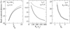 |
Fig. 1. Fraction of input photons that are back-scattered (dashed lines) and also illuminate the accretion disk (solid lines) as a function of optical depth (left panel), jet width (middle panel), and the Lorentz factor (right panel). |
It is evident from the left panel of Fig. 1 that, for reasonable values of the optical depth τ∥, the large majority of photons escape in such directions that they will not encounter the disk, which is expected. What is interesting is that a significant fraction of the escaping photons go back to the disk, despite the bulk motion of the electrons in the jet that tends to push them in the forward direction. The fraction of back-scattered photons increases with optical depth, and the relatively low bulk velocity in the acceleration zone helps. The fraction of back-scattered photons (dashed line) is slightly larger than that of those that hit the disk (solid line), and this is expected too.
In the middle panel of Fig. 1, we show the dependence of the back-scattered photons on the size of the jet, as measured by the radius R0 at its base. An increase in R0 results in a decrease in the back-scattered fraction, albeit a small one. For an increase by a factor of six in R0, the back-scattered fraction decreases by ∼5% (dashed line), while the fraction that hits the disk decreases by ∼10% (solid line).
In the right panel of Fig. 1, one can see the dependence of the back-scattered photons on the Lorentz factor γ0 of the electrons in the coasting region of the flow (z > z1). The variation of γ0 is due to the variation of the flow speed v0, and v⊥ is kept constant. As expected, the fraction of back-scattered photons decreases rapidly with increasing γ0. The leveling off at large γ0 may seem unphysical, but it is due to the scatterings that occur in the acceleration zone. Irrespective of the final v0, the parallel velocity is significantly smaller than v0 in the lower parts of the acceleration zone, and hence there are no large variations of the Lorentz factor for the cases considered in Fig. 1 in this region.
3.2. Height distribution of back-scattered photons
We now examine the percentage of photons that have back-scattered and hit the accretion disk as a function of the height h of the point of last scattering. The height distribution (Fig. 2) is characterized by a sharp peak at a low height (within a few gravitational radii), an extended plateau, and a high-height cutoff. In our jet model, Comptonization can occur anywhere in the jet (not only at its base). Thus, it is not surprising to see photons escaping from a large range of heights.
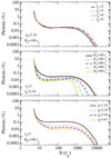 |
Fig. 2. Fraction of input photons that illuminate the disk as a function of the height h from where they escape the jet. |
Figure 2 shows the results of running different models with different optical depth τ∥, jet width R0, and Lorentz factor γ0. In each model, we vary one parameter and keep the other two at reasonable values. The results can be summarized as follows: (i) the height distribution does not depend strongly on optical depth (top panel), (ii) the cutoff at high h moves to smaller values as R0 increases (middle panel), and (iii) as γ0 increases, the fraction of the photons back-scattered toward the disk at every h decreases (bottom panel).
3.3. Spectrum of the back-scattered photons
Having demonstrated that a significant fraction of Comptonized photons move back toward the disk, we computed their spectrum. Figure 3 compares the spectrum of the photons that illuminate the disk, the “disk” spectrum (solid line), with the “direct” spectrum of the photons seen by observers at angles θ, with respect to the jet axis, in the range 0.7 < cos θ ≤ 0.8 (dashed line) or, equivalently, for a source inclination of ∼40°. Both spectra can be fitted with power laws with a high-energy cutoff. The disk spectrum is clearly softer than the direct spectrum. We emphasize that the disk spectrum is not the spectrum of the reflected radiation. It simply represents the energy distribution of the photons that illuminate the disk.
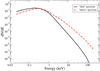 |
Fig. 3. Comparison of the “direct” and “disk” spectra. The direct spectrum is the spectrum seen by observers at infinity at an inclination θ, and the “disk” spectrum is the spectrum of the photons that are back-scattered and illuminate the disk. The direct spectrum was computed for 0.7 < cos θ ≤ 0.8). The parameters of the model used in this figure are: τ∥ = 3, R0 = 80 rg, and γ0 = 2.24. |
From the disk and the direct spectra, we can compute the ratio of the illuminating and the directly observed radiation. This ratio is generally known as the reflection fraction RF, although different authors give different definitions depending on whether the reflected flux, as opposed to the illuminating flux, is considered or whether relativistic (i.e., light-bending) effects are taken into account (see the appendix of Basak & Zdziarski 2016, for a detailed account of the reflection fraction). In the lamp post model, RF has been used to constrain the spin of the black hole (Dauser et al. 2014) and the geometry of the source of hard X-rays (Dauser et al. 2016).
Here we define RF simply as the ratio of the intensity that illuminates the disk to the intensity that directly reaches observers at infinity in a range of observing angles θ. The reflection fraction is then RF = Idisk/Idirect, where the intensities Idisk and Idirect are computed as
 (4)
(4)
where dN/dE is the number of photons per unit energy in the spectrum and the subscript i refers to either “disk” or “direct”. We calculated the reflection fraction in the energy range 1−100 keV, which is the range where the power law dominates. We divided the disk into 13 radial zones and computed the intensity of the photons that hit the disk between Ri and Rmax, where Ri is the inner radius of each zone. In other words, we mimicked the situation of a truncated disk whose inner radius decreases (i.e., the disk is approaching the black hole). We note that because the direct spectrum Idirect depends on the angle θ between the jet axis and the observer (Reig & Kylafis 2019; Kylafis et al. 2020), so does the reflection fraction.
In the computation of the reflection fraction, we ignored relativistic light-bending effects. In our model, we assume that photons are injected at the sides of the jet at its base. Because R0 is on the order of tens of gravitational radii, the number of photons that pass near the black hole is very small. Typically, the fraction of the input photons that enter the sphere r < 10 rg centered around the black hole is ≲0.01% for R0 ≳ 50 rg.
In Fig. 4, we show RF as a function of a disk inner radius for three different inclinations, 0.6 < cos θ ≤ 0.7 (i.e., θ ∼ 50°), 0.7 < cos θ ≤ 0.8 (i.e., θ ∼ 40°), and 0.8 < cos θ ≤ 0.9 (i.e., θ ∼ 30°). The RF increases as the inner disk radius Ri decreases, and it increases as the inclination of the system increases. The flat part of the curve reflects the fact that the inner parts of the disk are scarcely illuminated by back-scattered photons.
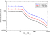 |
Fig. 4. Reflection fraction as a function of the inner radius for model parameters τ∥ = 3, R0 = 80 rg, and γ0 = 2.24. |
4. Discussion
The reflection spectrum results from the reprocessing of hard X-ray photons by the optically thick accretion disk. Therefore, we expect the properties of the illuminating radiation to have a profound impact on the spectral features of the reflection spectrum (Dauser et al. 2013; García et al. 2015; Steiner et al. 2017). Because of the complexity of the physics involved, many authors assume a static point source that emits isotropically, as in the lamp post model or coronal models (see, e.g., Vincent et al. 2016). In reality, the source is expected to be variable, extended, anisotropic, and partly off-axis (Dauser et al. 2013). Constraining the nature and geometry of the source of the hard X-rays that illuminates the disk will allow us to consider more realistic models. The aim of this work has been to investigate whether the jet itself can be the disk-illuminating source.
In this section, we discuss the process of disk illumination as well as the results obtained in the previous section. We have shown that a significant fraction of the photons return toward the accretion disk after being scattered in the jet. We have also determined the height at which the photons that are back-scattered toward the disk escape from the jet. Finally, we have computed the spectrum that illuminates the disk. Below, we elaborate on all three of these findings.
We have shown that, regardless of the optical depth, jet width, and jet velocity, a significant fraction of the Comptonized photons are back-scattered and hit the disk (Fig. 1). The decrease in the number of back-scattered photons as the optical depth decreases is expected because, for low optical depths, the photons find it easier to move along the jet and travel longer distances. The higher up in the jet they travel, the less likely it is for the back-scattered photons to hit the disk. Likewise, a larger outflow velocity of the electrons imposes a stronger forward motion on the photons and makes back-scattering more difficult. The decrease in the number of back-scattered photons as the jet width increases reflects the fact that photons can travel a longer distance along a wider jet before they escape via the sides of the jet; again, they are less likely to hit the disk.
An interesting result of our work is the height distribution of the photons that illuminate the disk. We have found that the majority of photons that hit the disk escape within a few gravitational radii, as expected in the lamp post model. The exact range of heights depends on our choice of the variable z0, which is the distance from the center of the base of the jet to the black hole. However, there is a significant contribution of photons that escape at larger radii (Fig. 2). The large fraction of back-scattered photons at small heights h is easily explained: In our model, we assume that photons are injected at the sides of the jet at its base. At the bottom of the jet, the optical depth is large (typically larger than 1). In addition, the flow velocity v∥ is small (the acceleration zone extends up to ∼50 rg). Hence, the photons do not experience a strong forward push. As a result, many photons escape after one (or very few) scattering(s) and do not travel long distances. The cutoff at high heights is also easily explained: As the height of the last scattering increases, the number of photons that hit the disk decreases because the solid angle that the disk subtends at this position decreases. Therefore, we expect a steep drop at high h, which is shown in Fig. 2. Finally, the plateaus seen in Fig. 2 are due to the fact that the optical depth in these regions is of order unity and the photons are scattered with equal probability there.
The height distribution is fairly insensitive to changes in optical depth τ∥. Large values of the optical depth parallel to the jet axis also imply large values of the optical depth perpendicular to the jet axis. The two effects compensate for each other, and photons travel more or less the same distance before they escape. Indeed, the ratio τ∥/τ⊥ as a function of h is about the same irrespective of the values of the optical depths. In contrast, the height cutoff decreases significantly as the jet width increases. This result can be explained by the fact that photons escape from the sides more easily in a narrow jet. As the width increases, more photons are able to travel along the jet before they escape from the sides. But, as mentioned above, the angle subtended by the disk becomes smaller as the escaping height increases. Hence, photons that escape at high heights have a high chance of missing the disk.
The explanation of why the back-scattered spectrum is softer than the forward, direct one is also quite simple. Consider soft photons entering a scattering region of an optical depth τ that is significantly larger than one. On average, the photons penetrate the scattering region one mean free path (i.e., optical depth equal to one). The photons that escape in the forward direction encounter an optical depth τ − 1, while the photons that are back-scattered encounter an optical depth of one. The photons that escape in the forward direction are scattered more times than the back-scattered ones and therefore gain more energy than the back-scattered ones. This is because, on average, the photons gain energy with every scattering. If there is bulk flow in the scattering region in the direction of the incoming photons, as is the case of a jet, then this effect is stronger because the photons are pushed in the forward direction by the bulk flow.
There is strong evidence that indicates that RF increases with luminosity (Plant et al. 2015; Basak & Zdziarski 2016; Steiner et al. 2016; Walton et al. 2017; Wang-Ji et al. 2018; Wang et al. 2020). This result is expected in the truncated disk model because, as the luminosity increases – that is to say, as the system moves from the hard state to the intermediate and soft states – the inner disk radius decreases (the disk moves inward), and hence the area irradiated in the disk increases. In Fig. 4, we naturally reproduce this trend.
Finally, there is the crucial question of whether there is any observational evidence for an extended and inhomogeneous lamp post. In this respect, García et al. (2019) showed that in order to achieve a good description of the reflected spectrum of GX 339–4, two sources of hard X-rays were needed: one located a few gravitational radii from the black hole and the second lying at h ∼ 600 rg. The second lamp post provided a better fit to the narrow component of the Fe K emission. Similarly, Chakraborty et al. (2020) obtained an improvement in the model that fitted the observed spectrum by considering a two-component corona at two different temperatures. This difference in coronal temperatures could be interpreted as originating from the fact that the two components are located at different distances from the black hole. The high-energy corona is much closer to the black hole and contributes to the broad iron line through blurred reflection, while the low-energy corona is farther away and contributes to the narrow core of the iron line complex. Basak & Zdziarski (2016) also found that, in the lamp post model, if the inner radius of the accretion disk is fixed to the ISCO, then the height of the source of hard X-rays is large (a few hundred rg).
The report of a number of discrete lamp posts most likely reflects the fact that the assumption of the lamp post model (an isotropic, stationary, point-like source) is an idealized case of the real physical source, which is likely extended, variable, and highly anisotropic (Dauser et al. 2013). Our model predicts a continuum of values of h at which the photons escape, and it appears to be a more natural and physical representation.
5. Conclusion
Comptonization in the jet is inescapable. The jet is fed from the hot inner flow. Thus, scattering in the hot inner flow, below the jet, will result in photons entering the jet and being scattered there as well. After all, the hot inner flow and the base of the jet have no boundary. Since in Comptonization it is the last scatterings that determine the outcome and not the first ones, scattering in the jet plays a fundamental role in shaping the radiation emitted by BHBs. We have shown that a significant fraction of photons that are Comptonized in a jet are back-scattered toward the accretion disk, despite the outward relativistic bulk velocity in the jet, and contribute to the illumination of the disk. The jet appears to be an excellent candidate for the source of hard X-rays in disk reflection models.
References
- Altamirano, D., & Méndez, M. 2015, MNRAS, 449, 4027 [NASA ADS] [CrossRef] [Google Scholar]
- Arévalo, P., & Uttley, P. 2006, MNRAS, 367, 801 [NASA ADS] [CrossRef] [Google Scholar]
- Bambi, C., Brenneman, L. W., Dauser, T., et al. 2020, ArXiv e-prints [arXiv:2011.04792] [Google Scholar]
- Basak, R., & Zdziarski, A. A. 2016, MNRAS, 458, 2199 [NASA ADS] [CrossRef] [Google Scholar]
- Belloni, T. M. 2010, in Lect. Notes Phys. (Berlin: Springer-Verlag), 794, 53 [NASA ADS] [CrossRef] [Google Scholar]
- Chakraborty, S., Navale, N., Ratheesh, A., & Bhattacharyya, S. 2020, MNRAS, 498, 5873 [CrossRef] [Google Scholar]
- Dauser, T., Garcia, J., Wilms, J., et al. 2013, MNRAS, 430, 1694 [NASA ADS] [CrossRef] [Google Scholar]
- Dauser, T., Garcia, J., Parker, M. L., Fabian, A. C., & Wilms, J. 2014, MNRAS, 444, L100 [NASA ADS] [CrossRef] [Google Scholar]
- Dauser, T., García, J., Walton, D. J., et al. 2016, A&A, 590, A76 [NASA ADS] [CrossRef] [EDP Sciences] [Google Scholar]
- Done, C., Gierliński, M., & Kubota, A. 2007, A&ARv, 15, 1 [NASA ADS] [CrossRef] [EDP Sciences] [Google Scholar]
- Duro, R., Dauser, T., Grinberg, V., et al. 2016, A&A, 589, A14 [NASA ADS] [CrossRef] [EDP Sciences] [Google Scholar]
- Emmanoulopoulos, D., Papadakis, I. E., Dovčiak, M., & McHardy, I. M. 2014, MNRAS, 439, 3931 [NASA ADS] [CrossRef] [Google Scholar]
- Esin, A. A., McClintock, J. E., & Narayan, R. 1997, ApJ, 489, 865 [NASA ADS] [CrossRef] [Google Scholar]
- Fabian, A. C., & Ross, R. R. 2010, Space Sci. Rev., 157, 167 [NASA ADS] [CrossRef] [Google Scholar]
- García, J. A., Dauser, T., Steiner, J. F., et al. 2015, ApJ, 808, L37 [NASA ADS] [CrossRef] [Google Scholar]
- García, J. A., Tomsick, J. A., Sridhar, N., et al. 2019, ApJ, 885, 48 [CrossRef] [Google Scholar]
- Kotov, O., Churazov, E., & Gilfanov, M. 2001, MNRAS, 327, 799 [NASA ADS] [CrossRef] [Google Scholar]
- Kylafis, N. D., & Reig, P. 2018, A&A, 614, L5 [NASA ADS] [CrossRef] [EDP Sciences] [Google Scholar]
- Kylafis, N. D., Papadakis, I. E., Reig, P., Giannios, D., & Pooley, G. G. 2008, A&A, 489, 481 [NASA ADS] [CrossRef] [EDP Sciences] [Google Scholar]
- Kylafis, N. D., Reig, P., & Papadakis, I. 2020, A&A, 640, L16 [CrossRef] [EDP Sciences] [Google Scholar]
- Lyubarskii, Y. E. 1997, MNRAS, 292, 679 [NASA ADS] [CrossRef] [Google Scholar]
- Martocchia, A., & Matt, G. 1996, MNRAS, 282, L53 [NASA ADS] [CrossRef] [Google Scholar]
- Martocchia, A., Matt, G., & Karas, V. 2002, A&A, 383, L23 [NASA ADS] [CrossRef] [EDP Sciences] [Google Scholar]
- McClintock, J. E., & Remillard, R. A. 2006, in Black Hole Binaries, eds. W. H. G. Lewin, & M. van der Klis, 157 [Google Scholar]
- Miniutti, G., Fabian, A. C., Goyder, R., & Lasenby, A. N. 2003, MNRAS, 344, L22 [NASA ADS] [CrossRef] [Google Scholar]
- Plant, D. S., Fender, R. P., Ponti, G., Muñoz-Darias, T., & Coriat, M. 2015, A&A, 573, A120 [NASA ADS] [CrossRef] [EDP Sciences] [Google Scholar]
- Pottschmidt, K., Wilms, J., Nowak, M. A., et al. 2003, A&A, 407, 1039 [NASA ADS] [CrossRef] [EDP Sciences] [Google Scholar]
- Rapisarda, S., Ingram, A., & van der Klis, M. 2017, MNRAS, 472, 3821 [CrossRef] [Google Scholar]
- Reig, P., & Kylafis, N. D. 2015, A&A, 584, A109 [NASA ADS] [CrossRef] [EDP Sciences] [Google Scholar]
- Reig, P., & Kylafis, N. D. 2019, A&A, 625, A90 [CrossRef] [EDP Sciences] [Google Scholar]
- Reig, P., Kylafis, N. D., Papadakis, I. E., & Costado, M. T. 2018, MNRAS, 473, 4644 [NASA ADS] [CrossRef] [Google Scholar]
- Reynolds, C. S. 2014, Space Sci. Rev., 183, 277 [Google Scholar]
- Saikia, P., Russell, D. M., Bramich, D. M., et al. 2019, ApJ, 887, 21 [CrossRef] [Google Scholar]
- Steiner, J. F., Remillard, R. A., García, J. A., & McClintock, J. E. 2016, ApJ, 829, L22 [NASA ADS] [CrossRef] [Google Scholar]
- Steiner, J. F., García, J. A., Eikmann, W., et al. 2017, ApJ, 836, 119 [NASA ADS] [CrossRef] [Google Scholar]
- Vignarca, F., Migliari, S., Belloni, T., Psaltis, D., & van der Klis, M. 2003, A&A, 397, 729 [NASA ADS] [CrossRef] [EDP Sciences] [Google Scholar]
- Vincent, F. H., Różańska, A., Zdziarski, A. A., & Madej, J. 2016, A&A, 590, A132 [CrossRef] [EDP Sciences] [Google Scholar]
- Walton, D. J., Mooley, K., King, A. L., et al. 2017, ApJ, 839, 110 [NASA ADS] [CrossRef] [Google Scholar]
- Wang, J., Kara, E., Steiner, J. F., et al. 2020, ApJ, 899, 44 [CrossRef] [Google Scholar]
- Wang-Ji, J., García, J. A., Steiner, J. F., et al. 2018, ApJ, 855, 61 [CrossRef] [Google Scholar]
- Zoghbi, A., Kalli, S., Miller, J. M., & Mizumoto, M. 2020, ApJ, 893, 97 [CrossRef] [Google Scholar]
All Figures
|
Fig. 1. Fraction of input photons that are back-scattered (dashed lines) and also illuminate the accretion disk (solid lines) as a function of optical depth (left panel), jet width (middle panel), and the Lorentz factor (right panel). |
| In the text | |
|
Fig. 2. Fraction of input photons that illuminate the disk as a function of the height h from where they escape the jet. |
| In the text | |
|
Fig. 3. Comparison of the “direct” and “disk” spectra. The direct spectrum is the spectrum seen by observers at infinity at an inclination θ, and the “disk” spectrum is the spectrum of the photons that are back-scattered and illuminate the disk. The direct spectrum was computed for 0.7 < cos θ ≤ 0.8). The parameters of the model used in this figure are: τ∥ = 3, R0 = 80 rg, and γ0 = 2.24. |
| In the text | |
|
Fig. 4. Reflection fraction as a function of the inner radius for model parameters τ∥ = 3, R0 = 80 rg, and γ0 = 2.24. |
| In the text | |
Current usage metrics show cumulative count of Article Views (full-text article views including HTML views, PDF and ePub downloads, according to the available data) and Abstracts Views on Vision4Press platform.
Data correspond to usage on the plateform after 2015. The current usage metrics is available 48-96 hours after online publication and is updated daily on week days.
Initial download of the metrics may take a while.