| Issue |
A&A
Volume 646, February 2021
|
|
|---|---|---|
| Article Number | A31 | |
| Number of page(s) | 12 | |
| Section | Numerical methods and codes | |
| DOI | https://doi.org/10.1051/0004-6361/202039624 | |
| Published online | 02 February 2021 | |
BAYES-LOSVD: A Bayesian framework for non-parametric extraction of the line-of-sight velocity distribution of galaxies⋆
1
Instituto de Astrofísica de Canarias, Vía Láctea s/n, 38205 La Laguna, Tenerife, Spain
e-mail: This email address is being protected from spambots. You need JavaScript enabled to view it.
2
Departamento de Astrofísica, Universidad de La Laguna, 38200 La Laguna, Tenerife, Spain
3
Astrophysics Research Institute, Liverpool John Moores University, 146 Brownlow Hill, Liverpool, L3 5RF, UK
e-mail: This email address is being protected from spambots. You need JavaScript enabled to view it.
Received:
9
October
2020
Accepted:
23
November
2020
Abstract
We introduce BAYES-LOSVD, a novel implementation of the non-parametric extraction of line-of-sight velocity distributions (LOSVDs) in galaxies. We employed Bayesian inference to obtain robust LOSVDs and associated uncertainties. Our method relies on a principal component analysis to reduce the dimensionality on the set of templates required for the extraction and thus increase the performance of the code. In addition, we implemented several options to regularise the output solutions. Our tests, conducted on mock spectra, confirm the ability of our approach to model a wide range of LOSVD shapes, overcoming limitations of the most widely used parametric methods (e.g., Gauss-Hermite expansion). We present examples of LOSVD extractions for real galaxies with known peculiar LOSVD shapes, including NGC 4371, IC 0719, and NGC 4550, using MUSE and SAURON integral-field unit (IFU) data. Our implementation can also handle data from other popular IFU surveys (e.g., ATLAS3D, CALIFA, MaNGA, SAMI).
Key words: methods: data analysis / techniques: spectroscopic / galaxies: general / galaxies: kinematics and dynamics / galaxies: elliptical and lenticular, cD / galaxies: spiral
Details of the code and relevant documentation are freely available in the dedicated repository: https://github.com/jfalconbarroso/BAYES-LOSVD
© ESO 2021
1. Introduction
Galaxies are made up of stars that move on orbits with different degrees of coherence around their nuclei. Each orbital group contains detailed information about the assembly history of each component and thus retains some memory of the different accretion events suffered by the galaxy over time. This information is encoded in their line-of-sight velocity distribution (LOSVDs), and thus by extracting this property we have access to vital clues to unravel the formation and evolution of galaxies we see today. The analysis of the LOSVD can be done directly in the Milky Way and in the local Universe by tracing the motions of stars with common stellar populations along a given line of sight (e.g., Norris 1986; Tolstoy et al. 2004; Deason et al. 2011; Kunder et al. 2012; Ness et al. 2013; Debattista et al. 2015; Zoccali et al. 2017; Du et al. 2020). This is a much more difficult task in nearby galaxies beyond the Local Group, where stars are unresolved and thus the LOSVD at a given position in a galaxy represents multiple populations along that line of sight.
The extraction of the LOSVD of galaxies has been an active field of research for many decades. Both parametric and non-parametric approaches have been developed over the years to address this issue. Interestingly, original implementations prioritised non-parametric over parametric recoveries, something that has radically changed in the last few decades. The most popular approaches include: Fourier correlation quotient (FCQ; Simkin 1974; Sargent et al. 1977; Franx & Illingworth 1988; Bender 1990); cross-correlation (XC or CCF; Tonry & Davis 1979; Statler 1995); maximum penalised likelihood (MPL; Saha & Williams 1994; Merritt 1997; Pinkney et al. 2003); and direct fitting in pixel space (e.g., Rix et al. 1992; Kuijken & Merrifield 1993; van der Marel & Franx 1993; Gebhardt et al. 2000; Kelson et al. 2000; Cappellari & Emsellem 2004; Ocvirk et al. 2006; Chilingarian et al. 2007).
The extraction of the LOSVD is a degenerate problem, as there are an indefinite number of combinations of stellar populations and LOSVD shapes that can explain a particular spectroscopic observation. Breaking the degeneracies implies perfect knowledge of the underlying stellar populations that contribute to a particular line of sight. In the last few decades, this issue has been mitigated with the advent of a large number of intermediate-resolution stellar libraries and stellar population models (see e.g., Bruzual & Charlot 2003; Valdes et al. 2004; Coelho et al. 2005; Sánchez-Blázquez et al. 2006; Prugniel et al. 2007; Vazdekis et al. 2010; Gonneau et al. 2020; Maraston et al. 2020) that have helped to greatly reduce the so-called effect of template mismatch (e.g., Falcón-Barroso et al. 2003). Another important aspect is the uncertainty of the recovered LOSVD. The methods cited above handle this in different ways. Most of them approach it using Monte Carlo simulations to perturb the input spectrum several times with some known observed uncertainty (however, see de Bruyne et al. 2003 for a more realistic approach). While in recent years the use of parametric forms of the LOSVD has prevailed in the literature (e.g., Emsellem et al. 2011; Falcón-Barroso et al. 2017; van de Sande et al. 2017), it is becoming increasingly clear that non-parametric approaches are needed to describe the complexity in the LOSVD shapes observed in real data (e.g., Jore et al. 1996; Kuijken et al. 1996; Halliday et al. 2001; González-García et al. 2006; Katkov et al. 2011; Coccato et al. 2013; Fabricius et al. 2014; Pizzella et al. 2018) and numerical simulations (e.g., Jesseit et al. 2007; Martig et al. 2014; Schulze et al. 2017).
Bayesian inference methods (e.g., Hoffman & Gelman 2014) offer a natural way of treating both: (1) the uncertainties in the fitting process, with the advantage that they allow the inclusion of our knowledge of the problem during the fitting process via priors on the input parameters; and (2) the true, complex, non-parametric nature of the LOSVDs. Saha & Williams (1994, hereafter SW94) already considered this particular way of framing the problem, but limitations in computer performance did not allow them to perform a fully general optimisation of both the LOSVDs and templates. In this paper, we revise the SW94 approach and use the latest developments on Bayesian inference and dimensionality reduction techniques to develop a Python1 implementation that can efficiently handle template optimisation and robust LOSVD extraction simultaneously.
The paper is organised as follows. We describe the problem of LOSVD extraction, the techniques for dimensionality reduction of the templates and LOSVD regularisation in Sect. 2. We present our tests on mock spectra in Sect. 3 and apply our extraction methods to real data in Sect. 5. We provide all the necessary technical details of our python implementation in Sect. 4, and provide a summary of the paper and outlook for future applications of this methodology in Sect. 6.
2. The LOSVD extraction
A LOSVD represents the distribution of the number of stars as a function of velocity along a particular line of sight in a galaxy. In spectroscopic data of nearby galaxies, the LOSVD is the broadening function to be applied to the spectrum of the underlying stellar populations. In essence, the extraction of the LOSVD is a deconvolution problem.
2.1. The equation
In its simplest form, the equation that describes the model to be fit to the data can be expressed in mathematical terms as:
![Mathematical equation: $$ \begin{aligned} G_{\rm model}\,(\lambda ) = \sum _{k=1}^{K} [w_k \cdot T_k(\lambda )] \star B + C(n), \end{aligned} $$](/articles/aa/full_html/2021/02/aa39624-20/aa39624-20-eq1.gif) (1)
(1)
where wk are the weights for each stellar population template (Tk), B is the broadening function (i.e. the LOSVD), the ⋆ operator is a convolution, and C(n) is an additive polynomial of order n. The polynomial term is convenient to reduce the impact of template mismatch (which can happen even with the most complete template libraries) and other imperfections during data reduction (e.g., non-perfect sky subtraction and/or scattered light). The equation can become more complicated if the effects of dust attenuation and/or calibration issues between data and templates are to be taken into account (see Eq. (11) in Cappellari 2017 for a more complete example). The implementation presented in this paper uses the prescription shown in Eq. (1), as we have checked that it works for a wide range of datasets, but it can be easily extended to include other correction terms if required.
The optimisation procedure involves the minimisation of the residuals:
 (2)
(2)
where xp is the value of the data or model at a given pixel, Gdata is the observed spectrum, ΔGdata are the observed uncertainties, and Gmodel is the model presented in Eq. (1). The most commonly used method for the minimisation of Eq. (2) is a least squares one, as there are plenty of computer implementations (e.g., Lawson & Hanson 1974; Moré et al. 2001; Jones et al. 2001) to perform the fits very efficiently.
Inspired by the work of SW94, we opted for revisiting their Bayesian non-parametric approach for the LOSVD extraction. There were three main aspects of SW94 that were not possible to explore given the computer capabilities and/or mathematical methods available at the time: (1) the Markov chain Monte Carlo (MCMC) sampling strategy; (2) template optimisation; and (3) different forms of regularisation for the LOSVD. We describe the new improvements in the following sections.
2.2. Markov chain Monte Carlo sampling
There are multiple possible strategies for the sampling of parameter space in Bayesian inference frameworks. Classical approaches include Metropolis-Hastings (Metropolis et al. 1953; Hastings 1970) or Gibbs (Geman & Geman 1984) samplers. With more complex models, the field has experienced a spur of new methods to efficiently probe large parameter spaces including nested sampling (e.g., Buchner 2016), Hamiltonian Monte Carlo (e.g., Duane et al. 1987), or Stein Variational Gradient Descent (e.g., Liu & Wang 2016) to cite a few. We refer the interested reader to Chi Feng’s Github webpage2 for a demo on the performance of different samplers.
The SW94 approach relied on the Metropolis algorithm for the exploration of parameter space. Our implementation is based on the No-U-Turn-Sampler (NUTS) introduced by Hoffman & Gelman (2014), that has proven to be a much more effective sampler. This is part of the Stan 3 package (Carpenter et al. 2017), which is our software of choice for the MCMC sampling. Stan is a probabilistic programming language for statistical modelling and data analysis used in many fields, from physics or engineering to social sciences. We refer the interested reader to Stenning et al. (2016), Asensio Ramos et al. (2017), Parviainen (2018), Lamperti et al. (2019), and Dullo et al. (2020) for a few examples of Stan applications in astronomy.
Besides the sampling scheme, one of the main advantages of our implementation within the Stan framework is the use of the simplex (i.e. a vector of positive values whose sum is equal to one) to describe the LOSVD. This type of parametrisation provides, naturally, physical and normalisation constraints, and it allows for a very efficient exploration of parameter space during minimisation (Betancourt 2012).
2.3. Template optimisation
A crucial element in the recovery of the LOSVD is the basis of stellar templates used to fit the observed spectra. Ideally, such a basis should contain stellar spectra covering the widest possible range of stellar parameters (i.e. Teff, [Fe/H], log(g), and stellar abundances) or stellar population models with a good sampling of, for example, ages, metallicities, IMF shapes and slopes, and possibly different chemical abundance ratios. As already mentioned in the introduction, this is now possible with the advent of the latest stellar libraries and models.
Using the typical set of ∼500−1000 templates, the minimisation involves finding the weights (wk) for each of them and performing the convolution of the LOSVD on ∼1000 spectral pixels per fitting iteration. This is a very time-consuming task even for the most efficient Bayesian samplers. Since reducing the number of pixels to fit may not be an option, we are thus left with the only alternative of decreasing the number of templates to be used in the optimisation process. This will have the advantage of not only reducing the number of parameters (i.e. wk), but also boosting minimisation performance by very large factors (e.g., from days to minutes).
There are a number of well-known techniques for dimensionality reduction that one could use to whittle down the number of templates: for example, independent component analysis (Lu et al. 2006), factor analysis (Nolan et al. 2006), non-negative matrix factorisation (Blanton & Roweis 2007), diffusion maps (Richards et al. 2009), or K-means (Sánchez Almeida & Allende Prieto 2013). Among all alternatives, we favoured the well-known principal component analysis (PCA) method. PCA has been extensively used in astrophysics for problems very much related to spectral fitting (e.g., Ronen et al. 1999; Li et al. 2005; Chen et al. 2012) and has proven to be both robust and very effective in speeding up calculations. With regard to our particular problem, the use of PCA has improved performance from several days to a few minutes (i.e. a 500-fold decrease in computing time).
In practice, the use of PCA means capturing well over 99% of the variance present in a template library of ∼1000 spectra with fewer than ten PCA components. Figure 1 shows the effect of using different numbers of PCA components during the fit for two mock spectra4 with a signal-to-noise ratio per pixel (hereafter S/N) of 50. It is remarkable how as few as two PCA components can already reproduce the observed spectrum with great accuracy. This is in part due to the use of additive polynomial that helps to reduce potential template mismatch issues. We checked the recovery for different types of stellar populations (as shown in the two columns), and the extracted LOSVD is less accurate for young stellar populations with a low number of PCA components. This is not unexpected given that spectra of younger populations show greater variation, which is difficult to capture with just two PCA components. We noticed that the closer the input spectrum is to the average spectra of the templates (i.e. intermediate stellar populations in our particular case), the better the recovery is for low number of PCA components. In general, our tests suggest that five PCA components suffice to recover the input LOSVD with great accuracy, with a clear improvement as S/N increases.
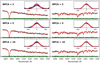 |
Fig. 1. Comparison of spectral fitting quality and LOSVD recovery for different numbers of PCA components. Each column presents input spectra with different stellar populations (young and old on the left and the right respectively). The input spectra have a S/N of 50 per pixel. All panels are plotted on the same scale. The black lines on the main panels are the input test data, while the red line shows the best fitting model. Residuals are indicated in green. The spectral fits are carried out with 2, 5, and 10 PCA templates (from top to bottom as indicated). In the insets, the input LOSVD is a Gaussian centred at zero and a velocity dispersion of 150 km s−1 (indicated in red). Units of the abscissae in the insets are km s−1. The recovered median values of the LOSVDs are indicated with a thick black line. 16%−84% and 1%−99% confidence limits at each point are indicated in dark and light blue, respectively. An order 2 auto-regressive prior was used to perform the fitting (see Sect. 2.4 for details). |
The optimal selection of the number of PCA components is not a well defined quantity, however. Choosing a number of PCA components that would explain a certain variance of the spectra (e.g., compatible with the noise of the spectrum) seems a reasonable approach. However, in practice, for real data this means selecting a different number of components for each spectrum of the dataset, which is very impractical. In our experience, for typical S/N ratios between 50 and 100, it is sufficient to choose a number between five and ten PCA components5. In our implementation, this number is a free parameter that the user has to decide on before runtime.
2.4. LOSVD regularisation
The extraction of the LOSVD is a degenerate problem with a large number of LOSVD shapes and combinations of templates that can reproduce the observed spectrum with great accuracy. Nevertheless, the range of allowed LOSVD solutions can be constrained for reasonably high S/N data.
There are different ways to impose some level of regularisation onto the output LOSVD. In our bayesian approach they are expressed in the form of priors over the LOSVD. We explored four different types of priors:
-
1.
No regularisation:
 (3)
(3)where LOSVDi is the ith velocity element of the LOSVD, and 𝒩(0, σ2) represents a normal distribution with mean zero and variance σ2. This is a fairly uninformative prior that assumes the same level of uncertainty on all LOSVD elements.
-
2.
Random-walk prior:
 (4)
(4)where the ith element of the LOSVD is linked to the previous one. This type of prior was the one proposed by SW94. We set the prior for the first element to LOSVD0 ∼ 𝒩(0, σ2).
-
3.
Auto-regressive prior:
 (5)
(5)This is a more general form of prior that becomes equal to the random-walk for α = 0 and β = 1 for k = 1. Stronger regularisation is obtained by increasing the order k, which links more consecutive LOSVD elements. We imposed the same prior used for the random-walk approach to the first element of the LOSVD, and used weakly informative normal priors for α and β.
-
4.
Penalised B-splines B-splines are a special type of piecewise polynomials controlled by knots that are often used for interpolation (e.g., Press et al. 2003). One of the major difficulties on the definition of B-splines is the choice of the number of knots to define the polynomial function. In our Stan implementation, we followed the example provided by Milad Kharratzadeh6, and rather than establishing a relation between different elements of the LOSVD, we applied random-walk priors to the B-spline coefficients such that
 (6)
(6)This approach promotes smoothness in the resulting LOSVD, preventing excessive wiggling in the solution. Another important parameter that controls the level of flexibility of the B-splines is the B-spline order k.
An interesting feature of our procedure is that we do not impose any pre-defined value to σ2 or τ during the fitting process. In fact, they are considered nuisance parameters, and we let the quality of the data establish their optimal distributions. Far from being unconstrained, it turns out that both parameters are well behaved and display fairly tight distributions.
We illustrate the effect of the choice of prior for the LOSVD and its uncertainties in Fig. 2. We created a test spectrum for this purpose with a Gaussian LOSVD and a S/N = 100 per spectral pixel. The figure shows the difference between no regularisation and an auto-regressive prior of order 2. Both approaches deliver an indistinguishable fit to the input spectrum and capture the Gaussian nature of the input LOSVD. However, the level of uncertainty displayed by the case without regularisation is far larger than that of the auto-regressive prior. These results are very much in agreement with the findings of Saha & Williams (1994). As we show in Sect. 3, this difference persists even at the highest S/N levels and is related to the number of degrees of freedom of one method versus the other.
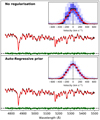 |
Fig. 2. LOSVD recovery for no regularisation and an auto-regressive (order 2) prior. Colours as in Fig. 1. |
2.5. Likelihood
Besides the priors, for the minimisation process, we need to define the form of the likelihood of our data given a model. In our problem, we assume that our spectroscopic observations can be explained by a normal distribution, such that
 (7)
(7)
where Gdata (λ) is the observed input spectrum, Gmodel (λ) is our model, and σGdata 2 is the variance of the observed spectrum.
Equation (1) is adequate to define our model when a full template library is to be used during the minimisation process. In our case, however, the use of PCA components transforms that equation to the following:
![Mathematical equation: $$ \begin{aligned} G_{\rm model}\,(\lambda ) = \left[\widetilde{T} + \sum _{k=1}^{K} w_k \cdot \mathrm{PCA}_k(\lambda )\right] \star B + C(n), \end{aligned} $$](/articles/aa/full_html/2021/02/aa39624-20/aa39624-20-eq8.gif) (8)
(8)
where wk are now the weights for each PCA component (PCAk),  is the mean template of the input library, B is the broadening function (i.e. the LOSVD), the ⋆ operator is a convolution, and C(n) is an additive polynomial of order n. Our implementation in Stan supports both forms of equations, but it is significantly more efficient with Eq. (8).
3. Tests on simulated data
We checked the performance of our implementation in different circumstances by creating mock spectra for a wide range of S/Ns and input LOSVD shapes. While some of the LOSVDs were arbitrarily defined by combining Gaussian functions, others come from numerical simulations and are thus more realistic. Here, we choose to illustrate a case with an input spectrum with an intermediate-age stellar population, but results are consistent when other populations were used. Our fits were performed using five PCA components.
Figure 3 shows an example of the recovery of an extreme case of LOSVD shape (i.e. a double-Gaussian profile) for a range of S/Ns and two prior assumptions. The effect of regularisation is evident from the lowest to the highest S/Ns. With no regularisation, there is a large range of possible solutions, as displayed by the confidence intervals, even at S/N = 200. It is interesting to note that the level of uncertainty decreases drastically with S/N when no regularisation is applied, while the improvement is not so large when priors are used. Regularised solutions come at the price of introducing some bias (see Sect. 5 for an example). This is most acute for the lowest S/Ns, where the regularised solution fails to capture the double-peaked nature of the input LOSVD. It is clear, however, that at S/N = 10, even non-regularised solutions cannot reproduce the input LOSVD. It seems that at an S/N of 25, the non-regularised solution already clearly reveals the double-peak feature, while the regularised one does not. This is an important result, as it shows that non-regularised solutions are more accurate at low S/N regimes, at the expense of larger uncertainties.
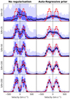 |
Fig. 3. LOSVD recovery for different S/Ns and types of regularisation. We used a double-Gaussian LOSVD profile as an example (indicated in red). Left column: solutions for extraction with no regularisation, right column: results for an order 2 auto-regressive prior. Each row represents two cases for a different S/N per pixel as indicated. All panels are plotted on the same scale. Colours as in Fig. 2. |
In Fig. 4, we present how the different types of regularisation methods listed in Sect. 2.4 influence the recovery of the range of input LOSVDs we prepared for these tests. The S/N of the input data is 50 per spectral pixel. The first thing to notice is that the overall level of accuracy in the LOSVD recovery is rather good (i.e. the input LOSVD is contained within the confidence levels) for all LOSVD shapes. Nevertheless, as expected from previous figures, the use of different priors result in different confidence intervals. An interesting feature is the difference in the confidence intervals between random-walk and auto-regressive (order 1) priors. This is entirely driven by the reduced number of degrees of freedom of the former compared to the latter (see Sect. 2.4). Perhaps one of the most important messages from the figure is that subtle details can be extracted at S/N = 50. This is particularly striking for the case displayed in the bottom row. This LOSVD is made of two Gaussians: a prominent one centred at −200 km s−1, and a faint component located at 500 km s−1. The goal of this test was to check the ability of the code to recover the presence of potential small satellites being accreted onto a galaxy. This appears to have been achieved for any choice of regularisation, with a slightly better recovery of the faint component with the random-walk and auto-regressive priors. These results are quite encouraging, as it means that there is no need for very high S/N ratios to detect this kind of feature. We provide versions of Fig. 4 for different S/Ns in Appendix A.
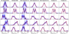 |
Fig. 4. LOSVD recovery for different input LOSVDs and types of regularisation. Colours as in Fig. 2. Each row represents a particular LOSVD shape for different types of regularisation. These are solutions for input spectra with S/N = 50 per pixel. All panels are plotted on the same scale. |
4. Implementation with pyStan
There are many alternatives one could choose from to implement all the ideas proposed in Sect. 2. Specifically, in Python some of the most popular packages include emcee7 (Foreman-Mackey et al. 2013) and pyMC38 (Salvatier et al. 2016), but we invite the reader to consult Gabriel Perren’s webpage9 for a comprehensive list of options. We picked pyStan10 as our package of choice to develop BAYES-LOSVD as it offers a convenient python interface to Stan.
BAYES-LOSVD is built in a modular fashion to make it very simple for the end user to extend its capabilities. This includes the addition of (1) read-in routines for data of a new instrument; (2) new Stan models with different kinds of regularisation; and (3) new template libraries. Our current implementation supports datacubes from the MUSE-WFM, SAURON, ATLAS3D, CALIFA, MaNGA, and SAMI surveys, as well as the possibility to read standard 2D FITS format files with spectra along the rows. The linearly sampled input spectra are pre-processed before execution, allowing the user to pick the level of Voronoi binning (using Cappellari & Copin 2003 implementation), the velocity range, and sampling of the output LOSVD. In this process, the designated templates will be prepared accordingly, with the possibility of switching off the reduction of the template basis with the PCA scheme described in Sect. 2.3.
Upon execution, the user can decide whether to analyse the entire set of Voronoi bins or a just a selection of them. Distributed computing is implemented natively, so that multiple spectra can be executed in parallel on multi-CPU machines. On output, by default, only summary statistics are stored. MCMC posterior distributions are described with highest density interval estimators (e.g., Kruschke 2014), which are more accurate to describe highly skewed distributions (as opposed to the standard percentiles approach). They are stored on disc in HDF5 format11. Diagnostic plots are also created if requested. Users wanting to delve into the details can chose to save the entire posterior distribution values, which can then be easily analysed using the Arviz12 package.
Performance and execution times depend very much on the data, and on the parameters used for the LOSVD extraction. Thanks to Stan, convergence is usually achieved with a very small number of iterations. In all the tests presented here, three chains with 500 iterations (i.e. warm-up + sampling) sufficed to obtain well-behaved posterior distributions. A typical spectrum with ∼500 pixels (e.g., 4800−5500 Å region) and S/N = 50 per pixel, a velocity range of ±700 km s−1 with a sampling of 50 km s−1, and five PCA components would require ∼10 min on a cluster with Intel Xeon E5-2630 (v4) CPUs.
There is one major bottleneck in our implementation: convolution is performed in direct space given Stan’s current inability to handle complex numbers. This has a very strong impact when wide spectral ranges are to be fitted. Based on discussions on the Stan forum13, we are aware that fast Fourier transforms will be possible in the not-so-distant future. Another aspect where we could already optimise performance is the likelihood evaluation. The latest version of Stan has introduced new features that can accelerate this process by large factors by distributing its computation over many CPUs. This is unfortunately not available in the pyStan version (v2.19) we are using, but it will be available with the release of pyStan (v3). Therefore, there is still room for performance improvements in the mid-term. We remain alert and will update the code to keep up with any new developments.
The code can be accessed via a dedicated Github repository14. Detailed documentation can be found on the same page.
5. Application to real data
We now turn our attention to the recovery of LOSVD using real data from different instruments. Here, we show examples of LOSVDs for three galaxies presenting LOSVDs with varying degrees of complexity. We chose data from MUSE-WFM and SAURON IFUs, but we note that the code has also been benchmarked with data from some of the most popular IFU surveys (e.g., ATLAS3D, CALIFA, MaNGA, SAMI).
5.1. NGC 4371
The first case we present is NGC 4371. This galaxy was studied in great detail by Gadotti et al. (2015) using the MUSE IFU, and it was part of the pilot programme for the TIMER survey (Gadotti et al. 2019). NGC 4371 is interesting as it is a fairly old system (i.e. ≥7 Gyr throughout) with evidence of a fossil nuclear stellar ring void of star formation (e.g., Erwin et al. 2001). Following the study of Gadotti et al. (2015), we extracted spectra with a 3.0″ aperture in three positions of the galaxy: at the centre, the nuclear stellar ring, and a location along the bar. The S/N of the spectra in the three apertures is well above 100 per pixel. We imposed a velocity sampling of 50 km s−1.
Figure 5 shows the results of our analysis. The three LOSVDs are different from each other in different aspects. While the LOSVDs at the centre and bar regions display fairly Gaussian profiles, the ring-dominated region is clearly asymmetric and skewed. The panels on the left-hand side show solutions with no regularisation, and the ones on the right used an order 2 auto-regressive prior. In essence, we see the same behaviour observed with the test data in previous sections with non-regularised solutions giving larger confidence intervals than the regularised ones. The two sets of solutions are very much consistent with each other, as was also observed in our experiments. These results presented in the figure were obtained by applying our method to spectra in the 4800−5300 Å wavelength range. We also computed solutions based on spectra around the calcium triplet region (8450−8700 Å) and obtained identical solutions (thus not shown here). This was not totally unexpected since there is no evidence of multiple stellar populations in this galaxy.
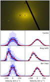 |
Fig. 5. BAYES-LOSVD extraction for NGC 4371. Top panel: Hubble Space Telescope colour image based on the F475W and F850LP filters. North is up and east to the left. Bottom panels: LOSVDs extracted at different locations (as indicated with black crosses on the image). On the left, without regularisation, and on the right with an order 2 auto-regressive prior. Colours as in Fig. 2. Red lines correspond to the best Gauss-Hermite LOSVD extracted with pPXF (see Sect. 5.1 for details). |
In addition, for comparison, we plot the best Gauss-Hermite LOSVD extracted with pPXF (Cappellari 2017). In this particular case, the agreement between the recovered LOSVDs with our method and pPXF is very good. This is especially true for the almost Gaussian LOSVDs at the centre and bar locations of the galaxy. At the ring, the regularised solution does not match the pPXF result as closely as the non-regularised one, but differences are still within a 1%−99% percentiles of our non parametric extraction. While for cases like this one, the advantage of the non-parametric approach may not seem evident, it is important to note that the Gauss-Hermite parametrisation allows for negative values on the wings of the LOSVD. This situation occurs for h3 and h4 values such as 0.1, and −0.1 respectively, which are not uncommon in the kinematic maps presented in many IFU surveys. Since we constrained the LOSVD during the fit to admit only positive values, our method overcomes this limitation and provides naturally physically meaningful LOSVDs.
5.2. IC 0719
The second case we studied was IC 0719, a spectacular case displaying multiple kinematic components (Katkov et al. 2013; Pizzella et al. 2018). This galaxy is made of stars in two counter-rotating large-scale discs with distinct stellar populations. In addition, it has an ionised gas component showing the same sense of rotation of the secondary, lower-mass, younger stellar disc. We used MUSE observations around the 4800−5300 Å region to extract three apertures along the major axis of the galaxy. As for the case of NGC 4371, the S/N of the spectra is well above 100 per pixel. We imposed a velocity sampling of 50 km s−1.
Figure 6 shows an almost perfect Gaussian LOSVD profile at the centre of the galaxy, while LOSVDs along the major axis display clear double-peaked shapes. This is in perfect agreement with the analysis performed by Pizzella et al. (2018). For comparison, we also plot the best-fit Gauss-Hermite LOSVD parametrisation obtained with pPXF (in red). Here, it becomes obvious that the Gauss-Hermite expansion cannot reproduce such complicated shapes well, and it shows LOSVD wings that have slightly negative values. Although not obvious due to the normalisation, for the aperture at 17″ the pPXF extraction creates a third peak in the LOSVD at velocities ∼500 km s−1, where the non-parametric approach goes effectively to zero. It is worth highlighting the level of complexity of the recovered LOSVDs despite the smooth morphological appearance. The same applies to NGC 4550, as we discuss in Sect. 5.3, and emphasises the need for the non-parametric LOSVD extraction in galaxies. This topic is gaining attention in the literature, and non-parametric LOSVDs are now being routinely included in the dynamical modelling of early-type galaxies (e.g., Mehrgan et al. 2019; Neureiter et al. 2021).
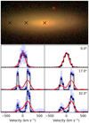 |
Fig. 6. BAYES-LOSVD extraction for IC 0719. Top panel: Sloan Digital Sky Survey colour image based on the g, r, i filters. The image has been rotated so that the major axis is parallel to the abscissae. Bottom panels: LOSVDs extracted at different locations along the major axis of the galaxy (as indicated with black crosses on the image). In the left column, without regularisation, and in the right one with an order 2 auto-regressive prior. Colours are the same as in Fig. 2. Red lines correspond to the best Gauss-Hermite LOSVD extracted with pPXF (see Sect. 5.2 for details). |
Another interesting aspect to explore in this galaxy is the non-parametric extraction of the LOSVD in wavelength regions sensitive to different stellar populations. This is actually possible with MUSE data, and it will be a subject of analysis in Rubino et al. (in prep.).
5.3. NGC 4550
The last case we analysed was NGC 4550, another classical showcase galaxy with prominent double-peaked LOSVD profiles. We extracted LOSVDs from SAURON spectra (Emsellem et al. 2004). We performed our calculations in the wavelength range between 4800−5300 Å and at a S/N = 150 per spectral pixel. We analysed the results along the major axis of the galaxy at three of the locations presented in Rix et al. (1992). Since their data were not in electronic form, we digitised them using the WebPlotDigitiser15 tool (Marin et al. 2017) and then fitted the LOSVDs with double-Gaussian profiles for best reproduction. Figure 7 (top panel) shows the F555W/F814W colour image from the Hubble Space Telescope. Remaining panels show our recovered LOSVDs at the three positions along the major axis, as indicated. Each row corresponds to a location, while each column uses different priors for the LOSVD extraction: no regularisation, auto-regressive (order 2), and auto-regressive (order 1). The red lines show the results of Rix et al. (1992).
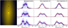 |
Fig. 7. BAYES-LOSVD extraction for NGC 4550. Left panel: Hubble Space Telescope colour image based on the F555W and F814W filters. North is up and east to the left. Other panels: LOSVDs extracted at several locations along the major axis of the galaxy (as marked by the black crosses). Each row corresponds to a different location from the centre of the galaxy (in arcsec) as shown on the first column. Each column uses a different kind of regularisation, as indicated in the top row. Colours are the same as in Fig. 2. Red lines show Rix et al. (1992) LOSVDs at those locations. |
The first thing to notice is the excellent agreement between our LOSVDs and those of Rix et al. (1992) when no regularisation is used. The complexity of the LOSVDs increases as we move away from the centre of the galaxy, as they become double-peaked from 7.6″. The results of Rix et al. (1992) are well within our 16%−84% confidence intervals (dark blue shaded region) despite the different sampling in velocity.
As opposed to IC 0719, the situation is drastically different when regularisation is applied, however. Our auto-regressive (order 2) solutions are not capable of capturing the double-peaked nature of the LOSVDs at larger distances from the centre. We investigated the source for this discrepancy and concluded that it is related to the intrinsic difference in velocity between the two peaks and the velocity sampling used to extract the LOSVDs. In other words, the level of correlation between velocity bins imposed by this prior is too strong and smooths the solution too much. In order to check this, we extracted the LOSVDs with an auto-regressive (order 1) prior, but we sampled the LOSVD in steps of 30 km s−1 instead of the 60 km s−1 used in all the other extractions. This is shown in the right-most column. It clearly shows that the two peaks can be recovered with a less stringent prior and finer sampling in velocity.
Based on these findings, we warn the reader that it is necessary to understand the implications of using regularisation in their analysis. We therefore recommend potential users to perform non-regularised fits on their data and carefully consider the velocity sampling to be used in the LOSVD extraction.
6. Summary and conclusions
The advent of very high quality data from many integral-field spectrographs and surveys has opened the possibility of efficiently extracting LOSVDs from galaxies. At the same time, great progress in computer performance, algorithms, and mathematical methods make it possible to handle large datasets. Inspired by the work of SW94, we developed a Bayesian inference approach to the LOSVD extraction from spectra. The code improves on SW94 in three main areas: (1) the MCMC sampling strategy; (2) the possibility of different forms of regularisation for the LOSVD; and (3) template optimisation based on PCA components. Our tests on mock data indicate that LOSVD recovery is accurate for spectra with S/N > 50 with as few as five PCA templates. Regularised solutions provide less uncertain LOSVDs, but it is at the expense of biased solutions for low S/Ns. We also successfully applied our approach to MUSE and SAURON data, displaying many interesting features and warning the users to be careful with regularised solutions in some situations (see Sect. 5.3 for an example). The use of non-regularised solutions should therefore be preferred, as it provides non-biased solutions.
On the technical side, our implementation is very versatile and allows the possibility of extending its capabilities on different fronts (i.e. inclusion of read-in routines for data of new instruments, new Stan models with different kinds of regularisation, and/or addition of new template libraries). The code and documentation can be downloaded from the repository indicated in Sect. 4.
The complexity in the kinematics observed in IFU surveys (e.g., Krajnović et al. 2011), but also numerical simulations (e.g., Martig et al. 2014; Schulze et al. 2017; Walo-Martín et al. 2020), clearly indicates that a non-parametric approach is necessary to capture the great level of detail that current data offer. This has been shown for decades in early-type galaxies, but the potential is much greater in late-type spiral systems, which display much more complex structures. In this respect, recent and upcoming large-scale IFU facilities (e.g., VIRUS-W, Fabricius et al. 2008; MEGARA, Gil de Paz et al. 2018 and WEAVE-LIFU, Dalton et al. 2018) operating at spectral resolutions above R ≥ 5000 open the door to explore the details of the LOSVDs in low velocity dispersion regimes (e.g., galaxy discs, dwarf galaxies), in which it has been very hard to operate with current instrumentation. The non-parametric description of the LOSVDs will also have a big impact on the decomposition of galaxies into their kinematic/dynamical components. Current efforts rely heavily on the smooth LOSVDs provided by Gauss-Hermite parametrisations (e.g., Tabor et al. 2017; Coccato et al. 2018; Oh et al. 2020). There is thus a great potential to go beyond those (necessary) efforts to explore galaxy mass assembly.
For reference, for this particular case, the continuum-to-line ratio (defined as 100 × σresiduals/σspectrum) is 13% and 23% for the young and old populations, respectively: almost independent of the number of PCA components used in the fitting procedure.
This is using the MILES models (Vazdekis et al. 2010).
Acknowledgments
We thank the referee Prasenjit Saha for very useful comments that have helped improving the manuscript. We are grateful to Prashin Jethwa, Ignacio Martín-Navarro, Marc Sarzi, Glenn van de Ven, and Eugene Vasiliev for many inspiring discussions over the course of this project. We are also indebted to Michela Rubino for her feedback and suggestions while testing earlier versions of the code, and Alireza Molaeinezhad for assisting in the preparation of the software package for Github. We thank Alessandro Pizzella for letting us use the IC 0719 MUSE datacube in our analysis. J. F.-B. thanks Andrés Asensio Ramos for introducing him to the world of bayesian inference methods and Stan in particular. We thank Michele Cappellari for letting us include some of his python functions in our software package. NGC 4371 results are based on observations collected at the European Southern Observatory under ESO programme 060.A-9313(A). Software acknowledgements. Our code uses Astropy (https://www.astropy.org/) a community-developed core Python package for Astronomy (Astropy Collaboration 2013, 2018), as well as NumPy (https://numpy.org/) (Oliphant 2006), SciPy (https://scipy.org/) (Jones et al. 2001) and Matplotlib (https://matplotlib.org/) (Hunter 2007). Funding and financial support acknowledgements. J. F.-B. acknowledges support through the RAVET project by the grant PID2019-107427GB-C32 from the Spanish Ministry of Science, Innovation and Universities (MCIU), and through the IAC project TRACES which is partially supported through the state budget and the regional budget of the Consejería de Economía, Industria, Comercio y Conocimiento of the Canary Islands Autonomous Community.
References
- Asensio Ramos, A., de la Cruz Rodríguez, J., Martínez González, M. J., & Socas-Navarro, H. 2017, A&A, 599, A133 [NASA ADS] [CrossRef] [EDP Sciences] [Google Scholar]
- Astropy Collaboration (Robitaille, T. P., et al.) 2013, A&A, 558, A33 [NASA ADS] [CrossRef] [EDP Sciences] [Google Scholar]
- Astropy Collaboration (Price-Whelan, A. M., et al.) 2018, AJ, 156, 123 [Google Scholar]
- Bender, R. 1990, A&A, 229, 441 [NASA ADS] [Google Scholar]
- Betancourt, M. 2012, in AIP Conf. Ser., eds. P. Goyal, A. Giffin, K. H. Knuth, & E. Vrscay, 1443, 157 [Google Scholar]
- Blanton, M. R., & Roweis, S. 2007, AJ, 133, 734 [NASA ADS] [CrossRef] [Google Scholar]
- Bruzual, G., & Charlot, S. 2003, MNRAS, 344, 1000 [NASA ADS] [CrossRef] [Google Scholar]
- Buchner, J. 2016, Stat. Comput., 26, 383 [CrossRef] [Google Scholar]
- Cappellari, M. 2017, MNRAS, 466, 798 [NASA ADS] [CrossRef] [Google Scholar]
- Cappellari, M., & Copin, Y. 2003, MNRAS, 342, 345 [NASA ADS] [CrossRef] [Google Scholar]
- Cappellari, M., & Emsellem, E. 2004, PASP, 116, 138 [NASA ADS] [CrossRef] [Google Scholar]
- Carpenter, B., Gelman, A., Hoffman, M., et al. 2017, J. Stat. Softw. Artic., 76, 1 [Google Scholar]
- Chen, Y.-M., Kauffmann, G., Tremonti, C. A., et al. 2012, MNRAS, 421, 314 [NASA ADS] [Google Scholar]
- Chilingarian, I., Prugniel, P., Sil’Chenko, O., & Koleva, M. 2007, in Stellar Populations as Building Blocks of Galaxies, eds. A. Vazdekis, & R. Peletier, IAU Symp., 241, 175 [Google Scholar]
- Coccato, L., Morelli, L., Pizzella, A., et al. 2013, A&A, 549, A3 [NASA ADS] [CrossRef] [EDP Sciences] [Google Scholar]
- Coccato, L., Fabricius, M. H., Saglia, R. P., et al. 2018, MNRAS, 477, 1958 [CrossRef] [Google Scholar]
- Coelho, P., Barbuy, B., Meléndez, J., Schiavon, R. P., & Castilho, B. V. 2005, A&A, 443, 735 [NASA ADS] [CrossRef] [EDP Sciences] [Google Scholar]
- Dalton, G., Trager, S., Abrams, D. C., et al. 2018, in Ground-based and Airborne Instrumentation for Astronomy VII, SPIE Conf. Ser., 10702, 107021B [Google Scholar]
- Deason, A. J., Belokurov, V., & Evans, N. W. 2011, MNRAS, 411, 1480 [NASA ADS] [CrossRef] [Google Scholar]
- Debattista, V. P., Ness, M., Earp, S. W. F., & Cole, D. R. 2015, ApJ, 812, L16 [NASA ADS] [CrossRef] [Google Scholar]
- de Bruyne, V., Vauterin, P., de Rijcke, S., & Dejonghe, H. 2003, MNRAS, 339, 215 [NASA ADS] [CrossRef] [Google Scholar]
- Du, H., Mao, S., Athanassoula, E., Shen, J., & Pietrukowicz, P. 2020, MNRAS, 498, 5629 [CrossRef] [Google Scholar]
- Duane, S., Kennedy, A. D., Pendleton, B. J., & Roweth, D. 1987, Phys. Lett. B, 195, 216 [NASA ADS] [CrossRef] [Google Scholar]
- Dullo, B. T., Bouquin, A. Y. K., Gil de Paz, A., Knapen, J. H., & Gorgas, J. 2020, ApJ, 898, 83 [CrossRef] [Google Scholar]
- Emsellem, E., Cappellari, M., Peletier, R. F., et al. 2004, MNRAS, 352, 721 [NASA ADS] [CrossRef] [Google Scholar]
- Emsellem, E., Cappellari, M., Krajnović, D., et al. 2011, MNRAS, 414, 888 [Google Scholar]
- Erwin, P., Vega Beltrán, J. C., & Beckman, J. E. 2001, in The Central Kiloparsec of Starbursts and AGN: The La Palma Connection, eds. J. H. Knapen, J. E. Beckman, I. Shlosman, & T. J. Mahoney, ASP Conf. Ser., 249, 171 [Google Scholar]
- Fabricius, M. H., Barnes, S., Bender, R., et al. 2008, in Ground-based and Airborne Instrumentation for Astronomy II, SPIE Conf. Ser., 7014, 701473 [CrossRef] [Google Scholar]
- Fabricius, M. H., Coccato, L., Bender, R., et al. 2014, MNRAS, 441, 2212 [NASA ADS] [CrossRef] [Google Scholar]
- Falcón-Barroso, J., Balcells, M., Peletier, R. F., & Vazdekis, A. 2003, A&A, 405, 455 [NASA ADS] [CrossRef] [EDP Sciences] [Google Scholar]
- Falcón-Barroso, J., Lyubenova, M., van de Ven, G., et al. 2017, A&A, 597, A48 [NASA ADS] [CrossRef] [EDP Sciences] [Google Scholar]
- Foreman-Mackey, D., Hogg, D. W., Lang, D., & Goodman, J. 2013, PASP, 125, 306 [Google Scholar]
- Franx, M., & Illingworth, G. D. 1988, ApJ, 327, L55 [NASA ADS] [CrossRef] [Google Scholar]
- Gadotti, D. A., Seidel, M. K., Sánchez-Blázquez, P., et al. 2015, A&A, 584, A90 [NASA ADS] [CrossRef] [EDP Sciences] [Google Scholar]
- Gadotti, D. A., Sánchez-Blázquez, P., Falcón-Barroso, J., et al. 2019, MNRAS, 482, 506 [Google Scholar]
- Gebhardt, K., Richstone, D., Kormendy, J., et al. 2000, AJ, 119, 1157 [NASA ADS] [CrossRef] [Google Scholar]
- Geman, S., & Geman, D. 1984, IEEE Transactions on Pattern Analysis and Machine Intelligence, PAMI-6, 721 [Google Scholar]
- Gil de Paz, A., Carrasco, E., Gallego, J., et al. 2018, in Ground-based and Airborne Instrumentation for Astronomy VII, SPIE Conf. Ser., 10702, 1070217 [Google Scholar]
- Gonneau, A., Lyubenova, M., Lançon, A., et al. 2020, A&A, 634, A133 [NASA ADS] [CrossRef] [EDP Sciences] [Google Scholar]
- González-García, A. C., Balcells, M., & Olshevsky, V. S. 2006, MNRAS, 372, L78 [NASA ADS] [CrossRef] [Google Scholar]
- Halliday, C., Davies, R. L., Kuntschner, H., et al. 2001, MNRAS, 326, 473 [NASA ADS] [CrossRef] [Google Scholar]
- Hastings, W. K. 1970, Biometrika, 57, 97 [Google Scholar]
- Hoffman, M. D., & Gelman, A. 2014, J. Mach. Learn. Res., 15, 1593 [Google Scholar]
- Hunter, J. D. 2007, Comput. Sci. Eng., 9, 90 [NASA ADS] [CrossRef] [Google Scholar]
- Jesseit, R., Naab, T., Peletier, R. F., & Burkert, A. 2007, MNRAS, 376, 997 [NASA ADS] [CrossRef] [Google Scholar]
- Jones, E., Oliphant, T., Peterson, P., et al. 2001, SciPy: Open Source Scientific tools for Python, http://www.scipy.org/ [Google Scholar]
- Jore, K. P., Broeils, A. H., & Haynes, M. P. 1996, AJ, 112, 438 [NASA ADS] [CrossRef] [Google Scholar]
- Katkov, I., Chilingarian, I., Sil’chenko, O., Zasov, A., & Afanasiev, V. 2011, Balt. Astron., 20, 453 [Google Scholar]
- Katkov, I. Y., Sil’chenko, O. K., & Afanasiev, V. L. 2013, ApJ, 769, 105 [NASA ADS] [CrossRef] [Google Scholar]
- Kelson, D. D., Illingworth, G. D., van Dokkum, P. G., & Franx, M. 2000, ApJ, 531, 159 [NASA ADS] [CrossRef] [Google Scholar]
- Krajnović, D., Emsellem, E., Cappellari, M., et al. 2011, MNRAS, 414, 2923 [NASA ADS] [CrossRef] [Google Scholar]
- Kruschke, J. 2014, Doing Bayesian Data Analysis: A Tutorial with R, JAGS, and Stan (Academic Press) [Google Scholar]
- Kuijken, K., & Merrifield, M. R. 1993, MNRAS, 264, 712 [NASA ADS] [Google Scholar]
- Kuijken, K., Fisher, D., & Merrifield, M. R. 1996, MNRAS, 283, 543 [NASA ADS] [CrossRef] [Google Scholar]
- Kunder, A., Koch, A., Rich, R. M., et al. 2012, AJ, 143, 57 [NASA ADS] [CrossRef] [Google Scholar]
- Lamperti, I., Saintonge, A., De Looze, I., et al. 2019, MNRAS, 489, 4389 [Google Scholar]
- Lawson, C. L., & Hanson, R. J. 1974, Prentice-Hall Series in Automatic Computation (Englewood Cliffs: Prentice-Hall) [Google Scholar]
- Li, C., Wang, T.-G., Zhou, H.-Y., Dong, X.-B., & Cheng, F.-Z. 2005, AJ, 129, 669 [NASA ADS] [CrossRef] [Google Scholar]
- Liu, Q., & Wang, D. 2016, ArXiv e-prints [arXiv:1608.04471] [Google Scholar]
- Lu, H., Zhou, H., Wang, J., et al. 2006, AJ, 131, 790 [NASA ADS] [CrossRef] [Google Scholar]
- Maraston, C., Hill, L., Thomas, D., et al. 2020, MNRAS, 496, 2962 [CrossRef] [Google Scholar]
- Marin, F., Rohatgi, A., & Charlot, S. 2017, in SF2A-2017: Proceedings of the Annual Meeting of the French Society of Astronomy and Astrophysics, eds. C. Reylé, P. Di Matteo, F. Herpin, et al., 113 [Google Scholar]
- Martig, M., Minchev, I., & Flynn, C. 2014, MNRAS, 443, 2452 [NASA ADS] [CrossRef] [Google Scholar]
- Mehrgan, K., Thomas, J., Saglia, R., et al. 2019, ApJ, 887, 195 [CrossRef] [Google Scholar]
- Merritt, D. 1997, AJ, 114, 228 [NASA ADS] [CrossRef] [Google Scholar]
- Metropolis, N., Rosenbluth, A. W., Rosenbluth, M. N., Teller, A. H., & Teller, E. 1953, J. Chem. Phys., 21, 1087 [NASA ADS] [CrossRef] [Google Scholar]
- Moré, J., Garbow, B., & Hillstrom, K. 2001, User Guide for MINPACK-1. Argonne National Laboratory Argonne, IL, http://cds.cern.ch/record/126569 [Google Scholar]
- Ness, M., Freeman, K., Athanassoula, E., et al. 2013, MNRAS, 432, 2092 [NASA ADS] [CrossRef] [Google Scholar]
- Neureiter, B., Thomas, J., Saglia, R., et al. 2021, MNRAS, 500, 1437 [Google Scholar]
- Nolan, L. A., Harva, M. O., Kabán, A., & Raychaudhury, S. 2006, MNRAS, 366, 321 [NASA ADS] [CrossRef] [Google Scholar]
- Norris, J. 1986, ApJS, 61, 667 [NASA ADS] [CrossRef] [Google Scholar]
- Ocvirk, P., Pichon, C., Lançon, A., & Thiébaut, E. 2006, MNRAS, 365, 74 [Google Scholar]
- Oh, S., Colless, M., Barsanti, S., et al. 2020, MNRAS, 495, 4638 [CrossRef] [Google Scholar]
- Oliphant, T. E. 2006, A Guide to NumPy (USA: Trelgol Publishing), 1 [Google Scholar]
- Parviainen, H. 2018, Bayesian Methods for Exoplanet Science (Springer International Publishing AG), 149 [Google Scholar]
- Pinkney, J., Gebhardt, K., Bender, R., et al. 2003, ApJ, 596, 903 [NASA ADS] [CrossRef] [Google Scholar]
- Pizzella, A., Morelli, L., Coccato, L., et al. 2018, A&A, 616, A22 [CrossRef] [EDP Sciences] [Google Scholar]
- Press, W. H., Teukolsky, S. A., Vettering, W. T., & Flannery, B. P. 2003, Eur. J. Phys., 24, 329 [CrossRef] [Google Scholar]
- Prugniel, P., Soubiran, C., Koleva, M., & Le Borgne, D. 2007, ArXiv e-prints [arXiv:astro-ph/0703658] [Google Scholar]
- Richards, J. W., Freeman, P. E., Lee, A. B., & Schafer, C. M. 2009, ApJ, 691, 32 [NASA ADS] [CrossRef] [Google Scholar]
- Rix, H.-W., Franx, M., Fisher, D., & Illingworth, G. 1992, ApJ, 400, L5 [NASA ADS] [CrossRef] [Google Scholar]
- Ronen, S., Aragon-Salamanca, A., & Lahav, O. 1999, MNRAS, 303, 284 [NASA ADS] [CrossRef] [Google Scholar]
- Saha, P., & Williams, T. B. 1994, AJ, 107, 1295 [NASA ADS] [CrossRef] [Google Scholar]
- Salvatier, J., Wiecki, T. V., & Fonnesbeck, C. 2016, PeerJ Comput. Sci., 2, 55 [CrossRef] [Google Scholar]
- Sánchez Almeida, J., & Allende Prieto, C. 2013, ApJ, 763, 50 [NASA ADS] [CrossRef] [Google Scholar]
- Sánchez-Blázquez, P., Peletier, R. F., Jiménez-Vicente, J., et al. 2006, MNRAS, 371, 703 [NASA ADS] [CrossRef] [Google Scholar]
- Sargent, W. L. W., Schechter, P. L., Boksenberg, A., & Shortridge, K. 1977, ApJ, 212, 326 [NASA ADS] [CrossRef] [Google Scholar]
- Schulze, F., Remus, R.-S., & Dolag, K. 2017, Galaxies, 5, 41 [NASA ADS] [CrossRef] [Google Scholar]
- Simkin, S. M. 1974, A&A, 31, 129 [NASA ADS] [Google Scholar]
- Statler, T. 1995, AJ, 109, 1371 [NASA ADS] [CrossRef] [Google Scholar]
- Stenning, D. C., Wagner-Kaiser, R., Robinson, E., et al. 2016, ApJ, 826, 41 [CrossRef] [Google Scholar]
- Tabor, M., Merrifield, M., Aragón-Salamanca, A., et al. 2017, MNRAS, 466, 2024 [NASA ADS] [CrossRef] [Google Scholar]
- Tolstoy, E., Irwin, M. J., Helmi, A., et al. 2004, ApJ, 617, L119 [NASA ADS] [CrossRef] [Google Scholar]
- Tonry, J., & Davis, M. 1979, AJ, 84, 1511 [NASA ADS] [CrossRef] [Google Scholar]
- Valdes, F., Gupta, R., Rose, J. A., Singh, H. P., & Bell, D. J. 2004, ApJS, 152, 251 [NASA ADS] [CrossRef] [Google Scholar]
- van de Sande, J., Bland-Hawthorn, J., Fogarty, L. M. R., et al. 2017, ApJ, 835, 104 [NASA ADS] [CrossRef] [Google Scholar]
- van der Marel, R. P., & Franx, M. 1993, ApJ, 407, 525 [NASA ADS] [CrossRef] [Google Scholar]
- Vazdekis, A., Sánchez-Blázquez, P., Falcón-Barroso, J., et al. 2010, MNRAS, 404, 1639 [NASA ADS] [Google Scholar]
- Walo-Martín, D., Falcón-Barroso, J., Dalla Vecchia, C., Pérez, I., & Negri, A. 2020, MNRAS, 494, 5652 [CrossRef] [Google Scholar]
- Zoccali, M., Vasquez, S., Gonzalez, O. A., et al. 2017, A&A, 599, A12 [NASA ADS] [CrossRef] [EDP Sciences] [Google Scholar]
Appendix A: S/N trends
In this appendix, we present the equivalent figures to Fig. 4 for different S/Ns. It is evident that the LOSVD recovery worsens as S/N decreases. It is interesting to see that not all the features are captured well, even at S/N = 100 (e.g., small bump on the positive wing of the case in the bottom row in all figures).
All Figures
|
Fig. 1. Comparison of spectral fitting quality and LOSVD recovery for different numbers of PCA components. Each column presents input spectra with different stellar populations (young and old on the left and the right respectively). The input spectra have a S/N of 50 per pixel. All panels are plotted on the same scale. The black lines on the main panels are the input test data, while the red line shows the best fitting model. Residuals are indicated in green. The spectral fits are carried out with 2, 5, and 10 PCA templates (from top to bottom as indicated). In the insets, the input LOSVD is a Gaussian centred at zero and a velocity dispersion of 150 km s−1 (indicated in red). Units of the abscissae in the insets are km s−1. The recovered median values of the LOSVDs are indicated with a thick black line. 16%−84% and 1%−99% confidence limits at each point are indicated in dark and light blue, respectively. An order 2 auto-regressive prior was used to perform the fitting (see Sect. 2.4 for details). |
| In the text | |
|
Fig. 2. LOSVD recovery for no regularisation and an auto-regressive (order 2) prior. Colours as in Fig. 1. |
| In the text | |
|
Fig. 3. LOSVD recovery for different S/Ns and types of regularisation. We used a double-Gaussian LOSVD profile as an example (indicated in red). Left column: solutions for extraction with no regularisation, right column: results for an order 2 auto-regressive prior. Each row represents two cases for a different S/N per pixel as indicated. All panels are plotted on the same scale. Colours as in Fig. 2. |
| In the text | |
|
Fig. 4. LOSVD recovery for different input LOSVDs and types of regularisation. Colours as in Fig. 2. Each row represents a particular LOSVD shape for different types of regularisation. These are solutions for input spectra with S/N = 50 per pixel. All panels are plotted on the same scale. |
| In the text | |
|
Fig. 5. BAYES-LOSVD extraction for NGC 4371. Top panel: Hubble Space Telescope colour image based on the F475W and F850LP filters. North is up and east to the left. Bottom panels: LOSVDs extracted at different locations (as indicated with black crosses on the image). On the left, without regularisation, and on the right with an order 2 auto-regressive prior. Colours as in Fig. 2. Red lines correspond to the best Gauss-Hermite LOSVD extracted with pPXF (see Sect. 5.1 for details). |
| In the text | |
|
Fig. 6. BAYES-LOSVD extraction for IC 0719. Top panel: Sloan Digital Sky Survey colour image based on the g, r, i filters. The image has been rotated so that the major axis is parallel to the abscissae. Bottom panels: LOSVDs extracted at different locations along the major axis of the galaxy (as indicated with black crosses on the image). In the left column, without regularisation, and in the right one with an order 2 auto-regressive prior. Colours are the same as in Fig. 2. Red lines correspond to the best Gauss-Hermite LOSVD extracted with pPXF (see Sect. 5.2 for details). |
| In the text | |
|
Fig. 7. BAYES-LOSVD extraction for NGC 4550. Left panel: Hubble Space Telescope colour image based on the F555W and F814W filters. North is up and east to the left. Other panels: LOSVDs extracted at several locations along the major axis of the galaxy (as marked by the black crosses). Each row corresponds to a different location from the centre of the galaxy (in arcsec) as shown on the first column. Each column uses a different kind of regularisation, as indicated in the top row. Colours are the same as in Fig. 2. Red lines show Rix et al. (1992) LOSVDs at those locations. |
| In the text | |
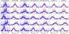 |
Fig. A.1. Same as Fig. 4, but for S/N = 10. |
| In the text | |
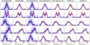 |
Fig. A.2. Same as Fig. 4, but for S/N = 25. |
| In the text | |
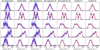 |
Fig. A.3. Same as Fig. 4, but for S/N = 100. |
| In the text | |
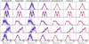 |
Fig. A.4. Same as Fig. 4, but for S/N = 200. |
| In the text | |
Current usage metrics show cumulative count of Article Views (full-text article views including HTML views, PDF and ePub downloads, according to the available data) and Abstracts Views on Vision4Press platform.
Data correspond to usage on the plateform after 2015. The current usage metrics is available 48-96 hours after online publication and is updated daily on week days.
Initial download of the metrics may take a while.