| Issue |
A&A
Volume 646, February 2021
|
|
|---|---|---|
| Article Number | A44 | |
| Number of page(s) | 6 | |
| Section | Astronomical instrumentation | |
| DOI | https://doi.org/10.1051/0004-6361/202039275 | |
| Published online | 04 February 2021 | |
Parameterized reconstruction with random scales for radio synthesis imaging
1
College of Big Data and Information Engineering, Guizhou University, Guiyang 550025, PR China
e-mail: This email address is being protected from spambots. You need JavaScript enabled to view it.
2
Xinjiang Astronomical Observatory, Chinese Academy of Sciences, Urumqi 830011, PR China
3
Key Laboratory of Radio Astronomy, Chinese Academy of Sciences, Urumqi 830011, PR China
4
Key Laboratory of Solar Activity, National Astronomical Observatories, Chinese Academy of Sciences, Beijing 100101, PR China
5
Center for Astrophysics, Guangzhou University, Guangzhou 510006, PR China
Received:
27
August
2020
Accepted:
7
December
2020
Abstract
Context. In radio interferometry, incomplete sampling results in a dirty beam with side lobes, which obscures the celestial structures. Before the astrophysical analysis, the effects of the dirty beam need to be eliminated, which can be solved with various deconvolution methods.
Aims. Diffuse astronomical sources observed by modern high-sensitivity telescopes tend to be complex morphological structures, often accompanied by faint features, which are submerged under the side lobes of the dirty beam. We propose a new deconvolution algorithm called random multiscale estimator (RMS-Clean), which is mainly used to solve the difficult reconstruction of diffuse astronomical sources.
Methods. RMS-Clean models the sky brightness distribution as a linear combination of random multiscale basis functions whose scales are obtained by randomly perturbing a preset multiscale list. Random multiscale models are used to approximate the uncertain characteristics of the scales of complex astronomical sources.
Results. When the RMS-Clean method is applied to simulations of SKA observations with realistic diffuse structures, it can reconstruct diffuse structures well and provides a competitive result compared to the commonly used deconvolution algorithms.
Key words: methods: data analysis / techniques: image processing
© ESO 2021
1. Introduction
The Square Kilometre Array (SKA; Dewdney et al. 2009; Wu 2019) is the world’s largest propopsed radio telescope, with very high sensitivity and a very large field of view. This telescope is likely to bring revolutionary changes to many fields of astronomy. However, the limited number of antennas often lead to incomplete sampling, which is nonuniformly distributed in the spatial frequency domain because of the nonuniform array configuration and the Earth-rotation aperture synthesis. This will produce non-negligible side lobes in the point spread function (PSF), which causes the details of the astronomical sources to be degraded to various degrees. Reconstructing astronomical sources from a dirty image is one of the main challenges of radio synthesis imaging, and deconvolving the PSF effect is the key technology.
In order to reconstruct the details of astronomical sources from a dirty image, many methods have been proposed. Because of noise and limited spatial frequency sampling, some prior information is required in the solution process to obtain the best results. The CLEAN-based algorithms (Högbom 1974; Zhang et al. 2020) are a class of methods for constructing parameterized models, which introduce scale priors. The zero-scale basis functions (i.e., delta functions) are used to construct the model for compact emission (Clark 1980). Scale basis functions such as Gaussians and tapered truncated parabolas are used to represent diffuse emission, which reflects the correlation between pixels in an astronomical image (Cornwell 2008; Zhang et al. 2016).
The maximum entropy method (MEM; Narayan & Nityananda 1986) is an explicit optimization process to use the entropy function as a regularizer. An entropy function is used to control model emission during reconstruction, and it is maximized to make the model more consistent with the measured data. The entropy function regularization is essential to obtain a smoothed version of the potential sky emission, as the smooth prior is used (Bhatnagar & Cornwell 2004).
In addition, compressive sensing (CS) methods are another type of optimization methods that often use regularizations. Unlike the MEM, a CS-based deconvolution method is based on the sparse assumption. CS theory posits that when the signal is sparse or can be sparsely represented in a certain domain, then a small number of samples can be used to recover the signal. This breaks through the sampling requirements of the Nyquist-Shannon theorem. In radio astronomy, compact emission is sparse in the image domain, and diffuse emission can become a sparse signal in the transformed domain. Wavelet transform is a sparse representation of the diffuse emission that is often used in the CS field. At the same time, CS often uses the L1 norm to find a more sparse solution and can apply many regularizations to obtain a model consistent with the regularizations, such as the sparsity averaging reweighted analysis (SARA; Carrillo et al. 2012), the sparse aperture synthesis interferometry reconstruction (SASIR; Girard et al. 2015) and model reconstruction by synthesis-analysis estimators (MORESANE; Dabbech et al. 2015).
Of these three types of deconvolution methods, MEM and CS are explicit optimization processes with regularization. MEM emphasizes smoothness, and CS emphasizes sparseness. Although the CLEAN-based method based on scale decomposition is simple, it can be well combined with other imaging procedures such as wide band and wide field. Among these methods, the CLEAN-based algorithms are more commonly used (Dabbech et al. 2015; Offringa & Smirnov 2017).
For modern high-sensitivity telescopes, diffuse emission, especially weak diffuse emission, makes reconstructing the sky emission difficult. In this article, we propose a new parametric deconvolution method with random scales, which is a random multiple scales estimator (RMS-Clean). The RMS-Clean aims to restore a better diffuse emission model.
To understand the RMS-Clean better, radio synthesis imaging and the deconvolution problems are introduced in Sect. 2. The theory of each part of the RMS-Clean and its algorithm process is introduced in Sect. 3. The experimental results and discussion are presented in Sect. 4, and the last section summarizes this work.
2. Deconvolution problems in radio synthesis imaging
In radio interferometry, the relation between the sky brightness distribution Isky and the visibility function Vsky in the measurement domain can be expressed as follows (Thompson et al. 2017):
 (1)
(1)
where w points along the direction of the light, (u, v) is its tangent plane, (l, m, n) defines the coordinate position of the source on the celestial sphere, and  . For small fields of view, this w-term can be ignored (Cornwell et al. 2008), which is also the case discussed in this paper.
In a real observation, factors such as the limited number of antennas, configuration of the array, observation time, and the channels determine the observed (u, v) coverage, which is the sampling function S(u, v), only measuring part of the visibilities. The measurement equation can be written as
 (2)
(2)
where N is the noise in the measurement domain such as the sky. The sampling function S(u, v) is composed of 1 for the sampled points and 0 for the unsampled points. As a result of factors such as Earth rotation synthesis, S(u, v) is not always on the grid points (i.e., noninteger coordinate points). Therefore Vobs is not always on the grid. In order to use technologies such as a fast Fourier transform to improve the computational efficiency, the measurement data need to be mapped onto grid points (Taylor et al. 1999; Thompson et al. 2017).
In matrix form, the measurement equation can be written as
![Mathematical equation: $$ \begin{aligned} V ^ \mathrm{obs} = [S] ([F] I ^ \mathrm{sky} + N), \end{aligned} $$](/articles/aa/full_html/2021/02/aa39275-20/aa39275-20-eq4.gif) (3)
(3)
where Vobs is the column vector representing the measured visibilities, [S] and [F] are the sampling matrix and Fourier transform matrix, respectively, Isky is the column vector for the sky brightness distribution, and N is the noise vector. Operations such as gridding have been ignored in the above measurement equation. In order to reconstruct the sky brightness distribution, the observed image (also called dirty image) Idirty needs to be calculated,
![Mathematical equation: $$ \begin{aligned} I ^ \mathrm{dirty} = [F ^ {\dag }] V ^ \mathrm{obs} = [F ^ {\dag } SF] I ^ \mathrm{sky} + n, \end{aligned} $$](/articles/aa/full_html/2021/02/aa39275-20/aa39275-20-eq5.gif) (4)
(4)
where [F†SF]Isky = [F†]([S][F]Isky)1 is a convolution of the PSF and the sky brightness distribution Isky, and n = [F†SF]N is the noise in the image plane.
The task now is to recover Isky from the dirty image degraded by the PSF and noise. With modern high-sensitivity telescopes, the observed images tend to be more complex structures. Effectively representing these complex structures is the key to the parameterized modeling method.
3. Parameterized deconvolution with random multiple scales
3.1. Multiscale model
An image with extended features tends to contain information of different scales. The pixels corresponding to source emission are clearly correlated within a scale. When a point-source model is used to represent these pixels, the correlation of pixels within the scale is omitted. The model is thus a linear combination of compact sources, which results in diffuse features that cannot be reconstructed well. Scale priors should be introduced to the representation of diffuse features. A multiscale model has been shown to represent diffuse emission better (Cornwell 2008; Rau 2010; Rau & Cornwell 2011).
In a multiscale model, the sky brightness distribution can be expressed as
 (5)
(5)
where ϵ is the error between the model image and true sky brightness distribution, which is an infinitesimal quantity only when the model image is consistent with the true sky brightness distribution. Such a model Imodel represents an image as a linear combination of Ns different scales,
 (6)
(6)
where  is a normalized scale function,
  is a location image composed of multiple δ functions, where the nonzero position represents the center position of the scale
  and the amplitude of each point represents the total flux of the scale. For compact sources, the magnitude of
  is itself. The asterisk stands for the convolution operation, which is usually implemented by fast Fourier transform,
![Mathematical equation: $$ \begin{aligned} I ^ \mathrm{model} = \sum _ {s = 0} ^ {N_ {s} -1} [F ^ {\dag } P_ {s} F] I_ {s} ^ {\delta -\mathrm{img}} , \end{aligned} $$](/articles/aa/full_html/2021/02/aa39275-20/aa39275-20-eq12.gif) (7)
(7)
where [Ps]=diag([F] ) is a diagonal matrix whose diagonal elements are given by [F]
 . Then the measurement equation can be written as
![Mathematical equation: $$ \begin{aligned} V ^ \mathrm{obs} = [S] ([F] (I ^ \mathrm{model} + \epsilon ) + N) = [SF] I ^ \mathrm{model} + [SF] \epsilon + [S] N. \end{aligned} $$](/articles/aa/full_html/2021/02/aa39275-20/aa39275-20-eq15.gif) (8)
(8)
Because the purpose of deconvolution is to model celestial sources, the noise item [S]N is ignored in the following discussion. In addition, the reconstructed error [SF]ϵ can be ignored in the absence of deconvolution errors. Combined with Eq. (7), the measurement equation can be expressed as follows:
![Mathematical equation: $$ \begin{aligned} V^\mathrm{obs} \approx V^\mathrm{model} = [SF]I^\mathrm{model} = \sum _{s = 0}^{N_{s} -1} [SP_{s} F] I_ {s} ^ {\delta -\mathrm{img}}, \end{aligned} $$](/articles/aa/full_html/2021/02/aa39275-20/aa39275-20-eq16.gif) (9)
(9)
where Vmodel is the visibilities of the model.
3.2. Multiscale model with random scales
Ps is clearly similar to a uv-taper function for nonzero scale sizes (Thompson et al. 2017), which suppresses high spatial frequencies and gives higher weights to lower spatial frequencies. When the size of a scale is greater than zero, this is equivalent to adjusting the sensitivity of the instruments to the peak value (Rau 2010). In the image plane, this is equivalent to constructing feature images of different scales.
In the commonly used multiscale method (Cornwell 2008; Rau & Cornwell 2011), the size of these scales is specified by the user, usually several. Then the sky brightness distribution needs to be expressed as a linear combination of these prespecified scales. Therefore these methods can only extract features of prespecified scales. The scale information contained in a sky brightness distribution cannot be known beforehand. If the scale of the features included in the sky brightness distribution is not consistent with the prespecified scales, it will be represented by the closest scale and leave the differences in residual structures. Based on this idea, as long as the scale is not the same as the prespecified scales, it will not represent the data well.
In order to solve this problem, we applied random multiscale mechanisms. A random multiscale model can be written in the following form:
 (10)
(10)
where Nsr is the number of random scales, and  and
and  are the scale basis function and location image with regard to the scale sr, respectively. The random multiscale method no longer uses the preset fixed scales only and its scales change randomly, which can effectively model the scale uncertainty of the sky brightness distribution. We implemented the random multiscale method by adding random perturbations to the preset scale list.
3.3. New algorithm
We introduce the details of the algorithm based on the above ideas. This algorithm uses the common image reconstruction framework in radio astronomy (Rau 2010; Zhang et al. 2020). Overall, the sky brightness distribution needs to be solved in the spatial frequency domain, and the solution needs to make the model consistent with the spatial frequency samples and be able to estimate the unmeasured points well. The estimation of the model is made in the image domain, which is the minor cycle. Error correction in the major cycle is made in the spatial frequency domain. The specific process is as follows:
1. Update scales and scale basis functions. The scale sr = ks is calculated based on the scales s ∈ {0, …, N} specified by the user, where k is a random perturbation coefficient that is a random number greater than zero. The maximum angular extent of resolvable emission for an interferometer provides a natural limit to the upper bound on k. Then sr is used to calculate a scale basis function  , which is a tapered and truncated parabola with sr.
2. Update the Hessian matrix. Calculate a Hessian matrix whose elements are given by  , where sr ∈ {0, …, N} and qr ∈ {0, …, N},
![Mathematical equation: $$ \begin{aligned} I_ {s_ {r}, q_ {r}} ^ {psf} = [F ^ {\dag } P_ {s_ {r}} P_ {q_ {r}} F] I ^ {psf}. \end{aligned} $$](/articles/aa/full_html/2021/02/aa39275-20/aa39275-20-eq22.gif) (11)
(11)
This is to calculate all possible pairs of scale basis functions, and store them first, and then use them to update the multiscale residual image for the model components, which can reduce time-consuming convolution calculations to reduce computational complexity.
3. Update multiscale residual images before model component estimation. Calculate the multiscale residual images for each current scale updated in step 1,
![Mathematical equation: $$ \begin{aligned} I_ {s_ {r}} ^ \mathrm{res} = [F ^ {\dag } P_ {s_ {r}} F] I ^ \mathrm{res}, \end{aligned} $$](/articles/aa/full_html/2021/02/aa39275-20/aa39275-20-eq23.gif) (12)
(12)
where Ires is the current residual image corresponding to zero scale, and the dirty image for the first time. After the scales are updated, the multiscale residual images need to be updated once from the current zero-scale residual image.
4. Estimate model components. Find the global peak value from these multiscale residual images, and obtain the principle solution by dividing by the corresponding peak value of the row element of the corresponding Hessian matrix. Here we can obtain the model component  , whose scale is
  centered at the nonzero value of the δ function and with the amplitude
  .
.
5. Update model. Update the current multiscale model image through the found model components,
![Mathematical equation: $$ \begin{aligned} I ^ \mathrm{model} = I ^ \mathrm{model} + g ([F ^ {\dag } P_ {q_ {r}} F] I_ {q_ {r}} ^ \mathrm{comp, \delta }), \end{aligned} $$](/articles/aa/full_html/2021/02/aa39275-20/aa39275-20-eq27.gif) (13)
(13)
where g is the loop gain, which ranges from 0 to 1, and is used to suppress overestimation.
6. Update multiscale residual images. The smoothed residual images for each scale are updated,
 (14)
(14)
Repeat the above steps 1–6 until the stop condition is met. Steps 1–6 contain a cycle, that is, steps 4–6 are repeated a certain number of times (e.g., five times) before the scales are updated again.
7. Predict model visibilities. When the root mean square (rms) limit or flux limit of the residual in the minor cycle is reached, the current model is predicted to the measurement domain,
![Mathematical equation: $$ \begin{aligned} V ^ \mathrm{model} = [A ^ {\dag }]I ^ \mathrm{model}, \end{aligned} $$](/articles/aa/full_html/2021/02/aa39275-20/aa39275-20-eq29.gif) (15)
(15)
where [A†] is the transform matrix from the image domain to the visibility domain, and is an inverse process of calculating the dirty image from the measurement data.
8. Update residuals from the spatial frequency domain. Calculate the visibility residuals and update the image-domain residuals,
![Mathematical equation: $$ \begin{aligned} I ^ \mathrm{res} = [A] (V ^ \mathrm{obs}-V ^ \mathrm{model}) . \end{aligned} $$](/articles/aa/full_html/2021/02/aa39275-20/aa39275-20-eq30.gif) (16)
(16)
Repeat the above steps until the sky emission is fully extracted.
Steps 1–6 are called the minor cycle, and steps 7–8 are called the major cycle. Steps 1–6 are used to construct the random multiscale model, while steps 7–8 can correct errors during model reconstruction. The final residual image is often added to the final reconstructed image, which ensures that the unreconstructed signal is not neglected, which is useful for data reconstruction such as very sparse sampling (e.g., very low baseline interferometry).
3.4. Implementation
When the scales are updated, the Hessian matrix needs to be recalculated, which involves multiple convolution operations. In our implementation, the scales and Hessian matrix are only randomly updated five times for each minor cycle to balance the computational load and the quality of the reconstructed image.
In this implementation, the zero scale must be included. It does not only model compact emission, but the residual corresponding to the zero scale is also used to calculate the multiscale residual images after the scales are updated. The latter can prevent the previous scale smoothing from accumulating in the next scale smoothing across major cycles.
In each component search, both the MS-Clean (Cornwell 2008) and RMS-Clean find the best value from multiple scales. The difference is that the RMS-Clean not only uses the preset scales, but also perturbs scales randomly. Compared with the Asp-clean algorithm (Bhatnagar & Cornwell 2004), unfixed scales are used to implement scale-adaptive modeling, but the ways of implementation are different. The asp-Clean uses the explicit fitting method to determine the largest scale of the current residuals, while the method in this paper is implemented in a random way. Each time, it determines the most suitable scale of the current multiple scales.
4. Results and discussion
In this section, SKA observations are simulated by the Radio Astronomy Simulation, Calibration and Imaging Library (RASCIL) software2 to verify the performance and motivation of the proposed algorithm, the RMS-Clean. These simulated observations were made with the core configuration of the SKA-Low array with a frequency of 100 megahertz and an observation bandwidth of 1 megahertz. In the first experiment, this realistic sky brightness distribution Cassiopeia A3 with complex morphological structures (i.e., the reference model image) (Fig. 1 left) was observed. The PSF formed by this observation is shown in the middle panel of Fig. 1. These side lobes are formed in the image domain by spatial frequencies that are not measured. This nonideal PSF obscures the details of the source in the observed Stokes-I image (called the dirty image, Figure 1 right). At the same time, the side lobes of the PSF make the dirty image with obvious side lobes in the nonsource region.
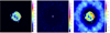 |
Fig. 1. Simulation results of SKA low-frequency observations. Left: reference model image Cassiopeia A. Middle: PSF displayed by the logarithmic scaling (CASA parameter “scaling power cycles” = −1.2) for more details of its sidelobes. Right: dirty image corrupted by the PSF. |
The results reconstructed by the proposed algorithm4 are shown in Fig. 2. The details of the source in the reconstructed model image (Fig. 2 top left) are significantly richer than those in the dirty image. The restored image (Fig. 2 bottom right) no longer contains the significant side-lobe structures of the nonsource area in the dirty image. The model error image (Fig. 2 top right), which is the difference between the reconstructed model image and the reference model image, contains only weak compact structures. This proves that the signal extraction in the dirty image is relatively sufficient, which is also verified by the weak structures in the residual image (Fig. 2 bottom left).
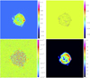 |
Fig. 2. Reconstruction results of source Cassiopeia A from the RMS-Clean algorithm. Top left: reconstructed model image. Top right: model error image, which is the difference between the reference model image and the reconstructed model image. Bottom left: residual image. Bottom right: restored image, which is the sum of the reconstructed model image convolved with the CLEAN beam and the final residuals. The specified scale list is [0, 7, 15, 22, 30] pixels that are randomly perturbed during the RMS-Clean deconvolution. The specified scale list can also be written as the relation between a scale list and the PSF main lobe, which has more physical meaning. For example, [0, 7, 15, 22, 30] pixels = [0, 3.3, 10.5, 14.3] × 2.1 pixels for this experiment. However, these two representations are completely equivalent because the PSF main lobe is a constant for a given experiment and only a common factor is extracted for the second representation. |
To further verify the RMS-Clean algorithm, a similar experiment was performed with source g215 (Fig. 3 top), and we compared this to the commonly used diffuse emission reconstruction method MS-Clean. The reconstruction results are shown in Fig. 4. Both methods can reconstruct the diffuse sources well (Fig. 4 top), but the RMS-Clean algorithm is more sufficient in extracting the signal so that the residual image contains fewer structures. The off-source rms and full rms of the RMS-Clean residual image are significantly smaller than those of the MS-Clean algorithm (Table 1). The dynamic range of the RMS-Clean restored image is also four times higher than that of MS-Clean (Table 1). A different structure source M87lo6 (Fig. 3 bottom) was simulated to further verify the performance of the RMS-Clean. This is consistent with the previous conclusion: the structures of the residual image are weaker and the dynamic range of the restored image is higher (Fig. 5 and Table 1). These experiments show that the RMS-Clean performs better than the commonly used MS-Clean (Tables 2 and 3).
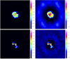 |
Fig. 3. Simulation results of sources g21 and M87lo. Top left: g21 reference model image. Top right: g21 dirty image. Bottom left: M87lo reference model image. Bottom right: M87lo dirty image. |
Numerical comparison of different algorithms for the g21 and M87lo simulations.
Numerical comparison of different specified scale lists for the g21 simulation.
Numerical comparison of different tests for reconstruction stability of random scales.
For the RMS-Clean deconvolution, we list some noteworthy features below.
1. The scale sizes in the RMS-Clean algorithm are randomly perturbed during the deconvolution process. It is found in experiments that the RMS-Clean algorithm more easily finds a better solution than the MS-Clean algorithm with a fixed scale list. The fixed scale list in the MS-Clean algorithm is more likely to fall into the local optimum in some cases. For example, a ring structure in the residuals during the deconvolution process has a small amplitude but a large scale size. The MS-Clean algorithm cannot easily escape this situation to obtain a global optimal solution. However, the RMS-Clean with random scales can quickly escape this point and find a new update direction to obtain a better reconstruction performance. Table 2 shows that the performance improvement of the RMS-Clean algorithm for different specified scale lists is visible, even when the scale list of the MS-Clean algorithm is “optimal”.
2. Compared with the MS-Clean, the deconvolution error ϵ of the RMS-Clean is smaller. This can be verified from the fewer structures in the residual images from a morphological point of view (see Figs. 4 and 5) and a lower rms (see Tables 1 and 2).
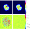 |
Fig. 4. Reconstruction results of source g21 from different algorithms. Top left: reconstructed model image from the MS-Clean algorithm. Top right: reconstructed model image from the RMS-Clean algorithm. Bottom left: residual image from the MS-Clean algorithm. Bottom right: residual image from the RMS-Clean algorithm. The specified scale list is [0, 7,15, 25, 40] pixels. |
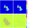 |
Fig. 5. Reconstruction results of source M87lo from different algorithms. Top left: reconstructed model image from the MS-Clean algorithm. Top right: reconstructed model image from the RMS-Clean algorithm. Bottom left: residual image from the MS-Clean algorithm. Bottom right: residual image from the RMS-Clean algorithm. The specified scale list is the same as Fig. 4. |
3. We have also observed some oscillations caused by the random scaling mechanism in the RMS-Clean algorithm in repeated experiments that do not use stored random perturbation coefficients (Table 3). However, each deconvolution can be accurately reproduced by the stored random perturbation coefficients. At the same time, this oscillation can be used to find a better solution by testing multiple times and using the criteria in Table 3 combined with the morphological features as other CLEAN algorithms.
4. The RMS-Clean has more scales, which can handle the scale uncertainty of the sky brightness distribution and obtain a better representation. However, MS-Clean can only represent the sky brightness distribution in a few fixed scales.
5. The scale randomness of the RMS-Clean algorithm is calculated by adopting a user-specified scale list and then randomly perturbing in the deconvolution process. Therefore RMS-Clean is very similar to the general MS-Clean in its use. This helps MS-Clean users to migrate to the RMS-Clean algorithm.
5. Summary
Modern high-sensitivity telescopes can observe weaker structures, and the observed sky brightness distribution tends to be more complicated. The dim and complex structures pose great challenges to the restoration of celestial brightness distributions. The introduction of multiscale parameterization of the sky brightness distribution can effectively represent the correlation between pixels within a scale. This improves the reconstruction quality of extended sources.
The existing multiscale methods model the sky brightness distribution as a linear combination of multiscale basis functions. The multiscale list needs to be specified by the user. Because of factors such as computational overhead and memory limit, only a few scale sizes usually employed. The sky brightness distribution is forcedly represented by these specified scales. The scale uncertainty of the sky brightness distribution means that such a representation leaves much compact emission, which requires many compact components to represent.
In this paper, a random multiscale method was introduced to solve the reconstruction problem of the scale uncertainty of the sky brightness distribution. The scales in the RMS-Clean vary randomly within a certain range by means of random perturbations. This cannot only deal with the uncertainty of the scale of the sky brightness distribution, but also increases the number of scales, which leads to an improved reconstruction quality. At the same time, it is also found by experiments that the random multiscale mechanism can help the deconvolution escape the local optimum, which causes the reconstruction to become a better solution.
In this paper, [R1R2R3]=[R1]([R2][R3]), that is, the order of operations is from right to left.
The RASCIL can be found from https://developer.skatelescope.org/projects/sim-tools/en/latest/ or https://github.com/SKA-ScienceDataProcessor/rascil, which is officially developed for radio interferometry imaging by the SKA organization.
https://public.nrao.edu/gallery/cassiopeia-a/, Credit: L. Rudnick, T. Delaney, J. Keohane & B. Koralesky.
The random perturbation coefficients k ∈ [0.5, 1.5) in these experiments.
https://public.nrao.edu/gallery/pulsar-wind-nebula/, Credit: NRAO /AUI/NSF and NASA/CXC.
https://www.nrao.edu/pr/1999/m87big/, credit: F.N. Owen, J.A. Eliek and N.E. Kassim.
Acknowledgments
The authors sincerely thank the anonymous referee for constructive advices. We would like to thank the people who have worked and are working on Python, RASCIL and CASA projects, which together built an excellent development and simulation environment. This work was partially supported by the National Natural Science Foundation of China (NSFC, 11963003, 61572461, 11790305, U1831204), the National SKA Program of China (2020SKA0110300), the National Key R&D Program of China (2018YFA0404602, 2018YFA0404603), the Guizhou Science & Technology Plan Project (Platform Talent No.[2017]5788), the Youth Science & Technology Talents Development Project of Guizhou Education Department (No.KY[2018]119,[2018]433]), Guizhou University Talent Research Fund (No.(2018)60) and “Light of West China” Programme (2017-XBQNXZ-A-008).
References
- Bhatnagar, S., & Cornwell, T. J. 2004, A&A, 426, 747 [NASA ADS] [CrossRef] [EDP Sciences] [Google Scholar]
- Clark, B. G. 1980, A&A, 89, 377 [NASA ADS] [Google Scholar]
- Cornwell, T. J. 2008, IEEE J. Sel. Top. Signal Process., 2, 793 [Google Scholar]
- Cornwell, T. J., Golap, K., & Bhatnagar, S. 2008, IEEE J. Sel. Top. Signal Process., 2, 647 [NASA ADS] [CrossRef] [Google Scholar]
- Carrillo, R. E., McEwen, J. D., & Wiaux, Y. 2012, MNRAS, 426, 1223 [NASA ADS] [CrossRef] [MathSciNet] [Google Scholar]
- Dabbech, A., Ferrari, C., Mary, D., et al. 2015, A&A, 576, A7 [NASA ADS] [CrossRef] [EDP Sciences] [Google Scholar]
- Dewdney, P., Hall, P., Schilizzi, R., & Lazio, T. 2009, Proc. IEEE, 97, 1482 [NASA ADS] [CrossRef] [Google Scholar]
- Högbom, J. A. 1974, A&AS, 15, 417 [Google Scholar]
- Girard, J. N., Garsden, H., Starck, J. L., et al. 2015, A&A, 575, A90 [NASA ADS] [CrossRef] [EDP Sciences] [Google Scholar]
- Narayan, R., & Nityananda, R. 1986, ARA&A, 24, 127 [NASA ADS] [CrossRef] [Google Scholar]
- Offringa, A. R., & Smirnov, O. 2017, MNRAS, 471, 301 [NASA ADS] [CrossRef] [Google Scholar]
- Rau, U. 2010, PhD Thesis, New Mexico Institute of Mining and Technology, Socorro, NM, USA [Google Scholar]
- Rau, U., & Cornwell, T. J. 2011, A&A, 532, A71 [NASA ADS] [CrossRef] [EDP Sciences] [Google Scholar]
- Taylor, G. B., Carilli, C. L., & Perley, R. A. 1999, in Synthesis Imaging in Radio Astronomy II, ASP Conf. Ser., 180 [Google Scholar]
- Thompson, A. R., Moran, J. M., & Swenaon, G. W. 2017, Interferometry and Synthesis in Radio Astronomy, 3rd Edn. (Springer) [Google Scholar]
- Wu, X. P. 2019, China SKA Science Report (Science press), ISBN: 9787030629791 [Google Scholar]
- Zhang, L., Bhatnagar, S., Rau, U., & Zhang, M. 2016, A&A, 592, A128 [NASA ADS] [CrossRef] [EDP Sciences] [Google Scholar]
- Zhang, L., Xu, L., & Zhang, M. 2020, PASP, 132, 041001 [CrossRef] [Google Scholar]
All Tables
Numerical comparison of different tests for reconstruction stability of random scales.
All Figures
|
Fig. 1. Simulation results of SKA low-frequency observations. Left: reference model image Cassiopeia A. Middle: PSF displayed by the logarithmic scaling (CASA parameter “scaling power cycles” = −1.2) for more details of its sidelobes. Right: dirty image corrupted by the PSF. |
| In the text | |
|
Fig. 2. Reconstruction results of source Cassiopeia A from the RMS-Clean algorithm. Top left: reconstructed model image. Top right: model error image, which is the difference between the reference model image and the reconstructed model image. Bottom left: residual image. Bottom right: restored image, which is the sum of the reconstructed model image convolved with the CLEAN beam and the final residuals. The specified scale list is [0, 7, 15, 22, 30] pixels that are randomly perturbed during the RMS-Clean deconvolution. The specified scale list can also be written as the relation between a scale list and the PSF main lobe, which has more physical meaning. For example, [0, 7, 15, 22, 30] pixels = [0, 3.3, 10.5, 14.3] × 2.1 pixels for this experiment. However, these two representations are completely equivalent because the PSF main lobe is a constant for a given experiment and only a common factor is extracted for the second representation. |
| In the text | |
|
Fig. 3. Simulation results of sources g21 and M87lo. Top left: g21 reference model image. Top right: g21 dirty image. Bottom left: M87lo reference model image. Bottom right: M87lo dirty image. |
| In the text | |
|
Fig. 4. Reconstruction results of source g21 from different algorithms. Top left: reconstructed model image from the MS-Clean algorithm. Top right: reconstructed model image from the RMS-Clean algorithm. Bottom left: residual image from the MS-Clean algorithm. Bottom right: residual image from the RMS-Clean algorithm. The specified scale list is [0, 7,15, 25, 40] pixels. |
| In the text | |
|
Fig. 5. Reconstruction results of source M87lo from different algorithms. Top left: reconstructed model image from the MS-Clean algorithm. Top right: reconstructed model image from the RMS-Clean algorithm. Bottom left: residual image from the MS-Clean algorithm. Bottom right: residual image from the RMS-Clean algorithm. The specified scale list is the same as Fig. 4. |
| In the text | |
Current usage metrics show cumulative count of Article Views (full-text article views including HTML views, PDF and ePub downloads, according to the available data) and Abstracts Views on Vision4Press platform.
Data correspond to usage on the plateform after 2015. The current usage metrics is available 48-96 hours after online publication and is updated daily on week days.
Initial download of the metrics may take a while.