© ESO 2021

1. Introduction

The study of Brownian motion was introduced in astrophysics by Chandrasekhar (1943a), who used it to establish, among other things, the concept of dynamical friction (Chandrasekhar 1943b). Brownian motion has also been used to model or estimate the motion of a massive black hole in the center of a stellar cluster or galaxy (Chatterjee et al. 2002a,b, 2003; Merritt 2005, 2013; Merritt et al. 2007; Bortolas et al. 2016; Lingam 2018; Di Cintio et al. 2020). While significant developments have been achieved regarding the statistical mechanics and a general kinetic theory of orbit-averaged motion in action-angle variables (Tremaine & Weinberg 1984; Binney & Lacey 1988; Chavanis 2012, 2013; Vasiliev 2017; Roupas et al. 2017; Fouvry & Bar-Or 2018; Tremaine 2020) or other canonical variables (Roupas 2020), a diffusion equation in configuration space for inhomogeneous Brownian motion – including varying velocity dispersion and diffusion coefficient – has not been applied as of yet. The paradigm of inhomogeneous Brownian motion is directly relevant to a self-gravitating system consisting of a population of heavier, fewer bodies immersed in a bigger, highly populated cluster of lighter bodies, whose profile is typically inhomogeneous regarding the density, velocity dispersion, and diffusion coefficient.

Such a population of a significant number of black holes (BHs) is believed to exist in the center of many globular clusters. Its existence is supported by numerical and theoretical developments (Merritt et al. 2004; Mackey et al. 2008; Morscher et al. 2013, 2015; Breen & Heggie 2013; Wang et al. 2016; Arca-Sedda 2016; Rodriguez et al. 2016; Chatterjee et al. 2017; Kremer et al. 2018, 2019; Askar et al. 2018; Arca Sedda et al. 2018; Weatherford et al. 2018, 2019) as well as observational evidence (Maccarone et al. 2007; Barnard et al. 2008; Strader et al. 2012; Irwin et al. 2010; Roberts et al. 2012; Chomiuk et al. 2013; Miller-Jones et al. 2015; Taylor et al. 2015; Minniti et al. 2015; Bahramian et al. 2017; Giesers et al. 2018; Shishkovsky et al. 2018; Abbate et al. 2019). These recent advances stand in contrast to a long-held belief that globular clusters cannot retain their BHs (Spitzer 1969; Kulkarni et al. 1993; Sigurdsson & Hernquist 1993). Spitzer instability (Spitzer 1969) seems unavoidable for massive stars which are subject to mass segregation, decoupling from the cluster and undergoing gravothermal collapse. The resulting black hole subcluster, according to a traditional view, would itself undergo core collapse and become so dense that would evaporate due to two-body and three-body encounters, apart from one or two BHs that may be retained in the centre (Kulkarni et al. 1993; Sigurdsson & Hernquist 1993). However, examining this picture more carefully, we may realize that since Spitzer instability depends on total mass and the BH-population has significantly less total mass than the progenitor subcluster of massive stars, the former might not undergo gravothermal collapse and might, instead, become stabilized. It has also been suggested that the BH-population does not stay decoupled from the cluster for as long a time as initially thought (Breen & Heggie 2013; Morscher et al. 2013).

Here, we propose an additional theoretical component to this picture. We investigate whether a BH-population that is well within the Spitzer instability regime may be supported by Brownian motion induced by the fluctuations of the cluster’s gravitational field. To this end, we describe the Brownian motion of the BHs due to fluctuations of the field by an inhomogenous diffusion equation that takes into account the density, velocity dispersion, and dynamical friction coefficient spatial variations. This model for the inhomogeneous diffusion of Brownian particles was discovered by van Kampen (1988) in a general setting and we argue that it also applies to self-gravitating systems.

In the next section, we review the Van Kampen inhomogeneous diffusion equation for Brownian particles and its stationary solution. In Sect. 2.1, we study a single massive BH and in Sect. 2.2, we consider a BH population immersed in a fixed Plummer profile. In the final section, we discuss our conclusions. In Appendix A, we re-derive the Van Kampen diffusion equation.

2. Inhomogeneous diffusion of black holes in stellar clusters

A standard approach in gravitational kinetic theory is to apply the orbit-averaged Fokker-Planck equation (e.g. Merritt 2013; Binney & Tremaine 2008). This approach comes with a drawback that Merritt (2013) ¹ refers to as a “kludge”. He remarks that while the diffusion coefficients are averaged over the volume filled by an orbit, no account is taken of the fact that the perturbations acting on a test star come from stars in regions far from the test star, which may have very different properties than those near to the test star. For this reason he concludes there is no sense in which the orbit-averaged Fokker-Planck equation might correctly describe an inhomogeneous system. We wish to describe the motion of heavier – that is, Brownian – bodies inside an inhomogeneous (in phase-space) medium of lighter bodies and, in addition, we wish to focus on the distribution of position. Therefore, we shall not use the standard orbit-averaged approach with E, L degrees of freedom, but the older approach from Chandrasekhar (1943b,a) in the phase-space x, v (see also Sect. 5.4 of Merritt 2013). We nevertheless generalize Chandrasekhar (1943a) approach here in order to account for inhomogeneity in space and temperature.

This may be achieved by considering the Kramers equation of the Fokker-Planck type (Kramers 1940) in a local sense (Eq. (A.3)) and derive a diffusion equation in a way that is similar to the derivation of the Smolukowski equation from the Kramers equation, as done by Chandrasekhar (1943a). This problem was already resolved by van Kampen (1988) and we provide a review in Appendix A.

Therefore, we suggest that the Van Kampen diffusion equation for Brownian motion in inhomogeneous media (van Kampen 1988) applies to self-gravitating systems, such as stellar clusters, which is the focus of this work, as well as dark matter haloes. These are typically spatially inhomogeneous and non-isothermal and they acquire a velocity dispersion that is also varying. If we denote μ(x) ≡ 1/mη(x), with η(x) as the diffusion coefficient and m the mass of a Brownian particle, Φ(x) and T(x) the potential and local temperature of the system in which the Brownian particle is embedded and p(x) the probability density of the Brownian particle in one dimenion x, the Van Kampen diffusion equation reads:

$$\begin{array}{c}\hfill \frac{\partial p(x,t)}{\partial t}=\frac{\partial }{\partial x}\left\{\mu (x)(m\mathrm{\Phi }{(x)}^{\prime }p(x,t)+\frac{\partial }{\partial x}(T(x)p(x,t)))\right\}.\end{array}$$(1)

As we noted above, we reproduce this equation in Appendix A. To be more specific, it is derived by expanding the Fokker-Planck Eq. (A.3) of Kramers with respect to η⁻¹, defined in the Langevin Eq. (A.5). This quantity is given in units of time and corresponds to the timescale of the diffusion, as was suggested by Chandrasekhar (1943b). Therefore, the Van-Kampen equation is strictly valid for times t ≫ η⁻¹.

The stationary distribution

$$\begin{array}{c}\hfill \frac{\partial p}{\partial t}=0\end{array}$$(2)

of Eq. (1) is

$$\begin{array}{c}\hfill p(x)=\frac{p(0)}{\beta (0)}\beta (x)e^{-{\int }_0^x\mathrm{d}\stackrel{\sim }{x}\beta (\stackrel{\sim }{x})m\mathrm{\Phi }{(\stackrel{\sim }{x})}^{\prime }},\end{array}$$(3)

where it is assumed that p(0)′ = T(0)′ = Φ(0)′ = 0. We denoted β = 1/T. In three dimensions, the diffusion Eq. (1) becomes

$$\begin{array}{c}\hfill \frac{\partial p(\mathit{r},t)}{\partial t}=\mathrm{\nabla }\left\{\mu (\mathit{r})(m(\mathrm{\nabla }\mathrm{\Phi }(\mathit{r}))p(\mathit{r},t)+\mathrm{\nabla }(T(\mathit{r})p(\mathit{r},t)))\right\}.\end{array}$$(4)

In the spherically symmetric case, the stationary radial probability density can therefore be written as

$$\begin{array}{c}\hfill p(r)=\frac{\beta (r)e^{-{\int }_0^r\mathrm{d}\stackrel{\sim }{r}\beta (\stackrel{\sim }{r})m\mathrm{\Phi }{(\stackrel{\sim }{r})}^{\prime }}}{{\int }_0^{\infty }\mathrm{d}r4\pi r^2\beta (r)e^{-{\int }_0^r\mathrm{d}\stackrel{\sim }{r}\beta (\stackrel{\sim }{r})m\mathrm{\Phi }{(\stackrel{\sim }{r})}^{\prime }}}·\end{array}$$(5)

The result is that at equilibrium, the probability density does not depend on μ(r), but only on β(r) and Φ(r). We note that the stationary phase space distribution function may be written at first order in η(x)⁻¹ by use of Eqs. (A.21), (A.23), and (A.27):

$$\begin{array}{cc}\hfill f(x,v)=& p(x)\sqrt{\frac{m}{2\pi T(x)}}{e}^{-\frac{m{v}^2}{2T(x)}}\hfill \\ \hfill & \times \{1-\eta {(x)}^{-1}\{v(\frac{1}{2}\frac{T{(x)}^{\prime }}{T(x)}p(x)+p{(x)}^{\prime })+v^3\frac{mT{(x)}^{\prime }}{T{(x)}^2}p(x)\}\}.\hfill \end{array}$$(6)

The temperature, T(x), refers to the host cluster. There a small correction term arises to the Maxwellian distribution. This requires further investigation and may be the subject of interesting future developments, but it is not discussed in this work.

2.1. Single black hole

Here, we consider a single BH of mass, m_b, as a Brownian particle immersed inside a stellar cluster of total mass, M_⋆, and average individual stellar mass, m_⋆.

We model the distribution of the stellar cluster with a Plummer sphere,

$$\begin{array}{cc}& {\rho }_{\star }(x)=\frac{M_{\star }}{\frac{4}{3}\pi r_{\mathrm{c}}^3}\frac{1}{{(1+x^2)}^{5/2}},{\mathcal{M}}_{\star }(x)=M_{\star }\frac{x^3}{{(1+x^2)}^{3/2}},\hfill \end{array}$$(7)

$$\begin{array}{cc}& {\sigma }_{\star }{(x)}^2=\frac{G{M}_{\star }}{6r_{\mathrm{c}}}\frac{1}{{(1+x^2)}^{1/2}},\hfill \end{array}$$(8)

where ρ_⋆(x), σ_⋆(x) denote the mass density and velocity dispersion of the host cluster, respectively, while ℳ_⋆(x) denotes the total stellar mass contained within x. The half-mass radius is related to the softening radius r_c by

$$\begin{array}{c}\hfill r_{\mathrm{hm}}={(2^{2/3}-1)}^{-1/2}{r}_{\mathrm{c}}\simeq 1.3r_{\mathrm{c}}.\end{array}$$(9)

We identify the temperature as

$$\begin{array}{c}\hfill T_{\star }(r)=m_{\star }{\sigma }_{\star }{(r)}^2.\end{array}$$(10)

The probability density of the BH position is given in a straightforward way from Eq. (5) which, in the case of Plummer external potential, may be written as

$$\begin{array}{c}\hfill p_{\mathrm{b}}=p_{\mathrm{b}}(0){(1+x^2)}^{-\frac{1}{2}-3\frac{m_{\mathrm{b}}}{m_{\star }}},\end{array}$$(11)

where

$$\begin{array}{c}\hfill p_{\mathrm{b}}(0)=\frac{1}{4\pi r_{\mathrm{c}}^3}\frac{4\mathrm{\Gamma }(3\frac{m_{\mathrm{b}}}{m_{\star }}+\frac{1}{2})}{\sqrt{\pi }\mathrm{\Gamma }(3\frac{m_{\mathrm{b}}}{m_{\star }}-1)},\end{array}$$(12)

and Γ is the gamma-function. In Fig. 1, we plot the probability density with respect to x for several different values of the individual mass ratio m_b/m_⋆. For a dense stellar cluster, such as a globular cluster or a nuclear star cluster, it is r_c ∼ 1−5 pc and m_⋆ ∼ 0.5 M_⊙. It is evident that an intermediate-mass BH with m_b ∼ 10³ M_⊙ inside a globular cluster wanders as far as ∼0.05 pc from the center, and in a nuclear star cluster, as far as ∼0.2 pc, although a Plummer sphere might not be a fairly good approximation for the density of the latter. A steeper external profile would induce smaller diffusion and, therefore, stricter boundaries for the BH fluctuation.

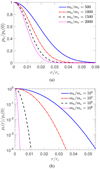Fig. 1. Stationary probability distribution pb of inhomogeneous diffusion (5) with respect to distance, r, for a single Brownian body, mb, inside a Plummer external gravitational potential. The Brownian body may be considered to be a massive BH and the gravitational potential may be generated by a globular cluster of individual average stellar mass, m⋆. We denote rc the softening radius of the potential.

In order to verify, in a straightforward manner, the validity of the inhomogeneous diffusion Eq. (1), we performed direct numerical N-body simulations using the AMUSE 13.2 framework (Portegies Zwart et al. 2009, 2013; Pelupessy et al. 2013; Portegies Zwart & McMillan 2018). We considered a stellar cluster with N_⋆ = 10³, m_⋆ = 0.5 M_⊙, r_c = 0.5 pc and a BH with m_b = 50 M_⊙ placed in the center of the cluster at distance r_b, ini = 1 AU and zero velocity. We use this initial condition for the BH to demonstrate that even if it is left sitting still in the center, it will eventually be kicked out due to gravitational fluctuations. In any case, we find that the distribution function seems to not be affected by the BH initial conditions, at least when it is initially bound inside the core ∼0.6r_c. We performed 1000 runs, initially sampling the stellar cluster from an isotropic Plummer phase-space distribution function f_Pl(x, v)∼(−E(x, v))^7/2. In our previous calculation (Eq. (11)), we assumed the Plummer potential to be fixed. Therefore, our sampling of the BH position should occur at a time is shorter than the relaxation time of the cluster t_rh = 0.138(N_⋆/lnΛ)(Gρ_⋆)^−1/2 (e.g., Heggie & Hut 2003; Portegies Zwart & McMillan 2018) so that the deviation from Plummer distribution is small. The relaxation time for a Plummer sphere is (Sect. 8, Table 1 of Heggie & Hut 2003):

$$\begin{array}{c}\hfill t_{\mathrm{rh}}=\frac{0.206}{ln\mathrm{\Lambda }}\frac{N_{\star }{r}_{\mathrm{c}}^{3/2}}{\sqrt{G{M}_{\star }}}=10\mathrm{Myr},\end{array}$$(13)

where we used Λ = 0.11N_⋆ (Portegies Zwart & McMillan 2018). The BH diffusion timescale t_b, rel is given from the two-body relaxation timescale (in a closely related context see El-Zant et al. 2020, 2016):

$$\begin{array}{c}\hfill t_{\mathrm{b},\mathrm{rel}}=\frac{1}{8\pi ln\mathrm{\Lambda }}\frac{{\sigma }_{\star }^3}{G^2{\rho }_{\star }{m}_{\mathrm{b}}}·\end{array}$$(14)

Dividing the two timescales, we get at the center r = 0:

$$\begin{array}{c}\hfill \frac{t_{\mathrm{b},\mathrm{rel}}}{t_{\mathrm{rh}}}=0.05\frac{m_{\star }}{m_{\mathrm{b}}}·\end{array}$$(15)

This verifies that the diffusion Eq. (1) is valid at times that are comparable to the relaxation timescale of a cluster for m_⋆ <  m_b. Now, for the parameters in our simulation, the last equation gives t_b, rel = 5 × 10⁻⁴t_rh = 5 × 10⁻³ Myr. We acquire the BH position at each simulation run within the time window, t = 0.3 ± 0.05 Myr, which is sufficiently bigger than t_b, rel, so that the BH has enough time to diffuse, and sufficiently smaller than t_rh, so that the Plummer potential does not get drastically altered.

We calculate the probability density by assuming the ergodic hypothesis holds (at each run, we record several positions in time) and performing an ensemble average. The fit of the theory of inhomogeneous diffusion to the simulations is very good, as depicted in Fig. 2. In Fig. 2a, we demonstrate in a single simulation run that the BH rapidly (at ∼t_b, rel = 0.005 Myr) diffuses in the medium, while in Fig. 2b, we present the BH probability density of 1000 simulation runs. The RMS position $r_{\mathrm{r}\mathrm{m}\mathrm{s}}\equiv ⟨r_{\mathrm{b}}^2{⟩}^{1/2}$ of the simulations $r_{\mathrm{rms}}^{\mathrm{sim}}=0.037$ pc is well-matched by the theoretical prediction $r_{\mathrm{rms}}^{\mathrm{theory}}=0.036$ pc in the chosen time window.

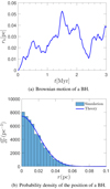Fig. 2. N-body simulations with AMUSE framework of a BH with mass mb = 50 M⊙ immersed with zero velocity in the center, rb, ini = 1 AU, of a stellar cluster with N⋆ = 1000, m⋆ = 0.5 M⊙, and initial conditions sampled from a Plummer sphere with softening radius, rc = 0.5 pc. (a) Radial position of the BH with respect to time in a single run. (b) Probability density of the position of the BH for 1000 runs. See text for details.

2.2. Black hole subcluster

Here, we consider a two-component model, namely a population of N_b Brownian particles with average mass, m_b embedded in a cluster of N_⋆ bodies with average mass, m_⋆. Our description wishes to describe a BH population immersed in a globular cluster, but applies generally to any self-gravitating system which hosts a subsystem of significantly less bodies. The total mass of the host is M_⋆ = N_⋆m_⋆ and the total mass of the Brownian bodies is M_b = N_bm_b.

The potential Φ includes the potential of the host cluster, but also can account for the self-gravity of the Brownian population if not negligible. Given the distribution of the host cluster and neglecting the feedback of the Brownian population onto the distribution of the host, the diffusion Eq. (1) together with the Poisson equation form a system of equations that determines the equilibrium distribution of the Brownian particles. This system may be formulated as follows. In the spherically symmetric case, the gravitational field at any point r may be decomposed according to Poisson equation as

$$\begin{array}{c}\hfill \frac{\mathrm{d}\mathrm{\Phi }}{\mathrm{d}r}=G\frac{{\mathcal{M}}_{\star }(r)+{\mathcal{M}}_{\mathrm{b}}(r)}{r^2},\end{array}$$(16)

where ℳ_⋆, ℳ_b denote the mass contained in r of the host cluster and the subcluster respectively. The equilibrium corresponds to the stationary solution of the inhomogeneous diffusion Eq. (1). We therefore get the system for the Brownian population:

$$\begin{array}{cc}& \frac{\mathrm{d}{p}_{\mathrm{b}}(r)}{\mathrm{d}r}=-p_{\mathrm{b}}(r)(G{m}_{\mathrm{b}}\frac{{\mathcal{M}}_{\star }(r)+{\mathcal{M}}_{\mathrm{b}}(r)}{r^2{T}_{\star }(r)}+\frac{T_{\star }{(r)}^{\prime }}{T_{\star }(r)}),\hfill \end{array}$$(17)

$$\begin{array}{cc}& \frac{\mathrm{d}{\mathcal{M}}_{\mathrm{b}}(r)}{\mathrm{d}r}=4\pi r^2{M}_{\mathrm{b}}{p}_{\mathrm{b}}(r).\hfill \end{array}$$(18)

This is a system of the unknown distributions {p_b, ℳ_b} given the host cluster distributions ℳ_⋆(r) and T_⋆(r) and subject to the constraint ℳ_b(∞) = M_b. The constraint suggests that equilibria may exist only for certain parameter values. This formulation, where the host cluster distribution is fixed, does not take into account the feedback of the Brownian population onto the host. This may be significant in the proximate regions close to the population if it is sufficiently compact, but we do not be consider this point in this work.

Supposing that the system is characterised by a length scale, r_c, we may introduce the dimensionless variables:

$$\begin{array}{cc}& x=\frac{r}{r_{\mathrm{c}}},{\stackrel{\sim }{M}}_{\mathrm{b}}(x)=\frac{{\mathcal{M}}_{\mathrm{b}}(x)}{M_{\mathrm{b}}},{\stackrel{\sim }{M}}_{\star }(x)=\frac{{\mathcal{M}}_{\star }(x)}{M_{\star }},\hfill \end{array}$$(19)

$$\begin{array}{cc}& {\stackrel{\sim }{p}}_{\mathrm{b}}(x)=4\pi r_{\mathrm{c}}^3{p}_{\mathrm{b}},y(x)=-ln\frac{{\stackrel{\sim }{p}}_{\mathrm{b}}(x)}{{\stackrel{\sim }{p}}_{\mathrm{b}}(0)}·\hfill \end{array}$$(20)

The system (17) and (18) becomes

$$\begin{array}{cc}& \frac{\mathrm{d}y(x)}{\mathrm{d}x}=\frac{G{m}_{\mathrm{b}}{M}_{\star }}{r_{\mathrm{c}}{T}_{\star }(x)}\frac{1}{x^2}({\stackrel{\sim }{M}}_{\star }(x)+\frac{M_{\mathrm{b}}}{M_{\star }}{\stackrel{\sim }{M}}_{\mathrm{b}}(x))+\frac{T_{\star }{(x)}^{\prime }}{T_{\star }(x)},\hfill \end{array}$$(21)

$$\begin{array}{cc}& \frac{\mathrm{d}{\stackrel{\sim }{M}}_{\mathrm{b}}(x)}{\mathrm{d}x}={\stackrel{\sim }{p}}_{\mathrm{b}}(0)x^2{e}^{-y(x)},\hfill \end{array}$$(22)

with initial conditions

$$\begin{array}{c}\hfill y(0)=0,{\stackrel{\sim }{M}}_{\mathrm{b}}(0)=0,y{(0)}^{\prime }=0,{\stackrel{\sim }{M}}_{\mathrm{b}}{(0)}^{\prime }=0\end{array}$$(23)

and subject to the boundary constraint

$$\begin{array}{c}\hfill {\stackrel{\sim }{M}}_{\mathrm{b}}(\infty )=1\iff {\stackrel{\sim }{p}}_{\mathrm{b}}(0)={\left({\displaystyle {\int }_0^{\infty }}\mathrm{d}x{x}^2{e}^{-y(x)}\right)}^{-1}.\end{array}$$(24)

For given host distributions M̃_⋆(x), T(x) the system (21)–(24) may be solved numerically.

We consider again the case where the stellar distribution is that of a Plummer sphere, as in Eq. (7). The temperature is identified as T_⋆(r) = m_⋆σ_⋆(r)². The system (21) and (22) becomes

$$\begin{array}{cc}& \frac{\mathrm{d}y(x)}{\mathrm{d}x}=6\frac{m_{\mathrm{b}}}{m_{\star }}(\frac{x}{1+x^2}+\frac{M_{\mathrm{b}}}{M_{\star }}\frac{\sqrt{1+x^2}}{x^2}{\stackrel{\sim }{M}}_{\mathrm{b}}(x))-\frac{x}{1+x^2},\hfill \end{array}$$(25)

$$\begin{array}{cc}& \frac{\mathrm{d}{\stackrel{\sim }{M}}_{\mathrm{b}}(x)}{\mathrm{d}x}={\stackrel{\sim }{p}}_{\mathrm{b}}(0)x^2{e}^{-y(x)},\hfill \end{array}$$(26)

subject again to the conditions (23) and (24).

The reach (or otherwise) of an equilibrium and the specific form of the equilibrium distribution of the Brownian particles, which we consider hereof to be a BH population, depend on both the number of bodies and their individual mass. In Fig. 3a, we calculate the series of equilibria of BH populations immersed in a Plummer stellar profile for various ratios m_b/m_⋆. Different points of each curve correspond to the equilibrium state of a different BH population with total mass, M_b, and corresponding central density p̃(0). We identify an instability that sets in at the maximum of the series of equilibria curve. No equilibria exist above the maximum, whereas, according to the Poincaré theorem of linear series of equilibria, the branch beyond the turning point (dotted lines in Fig. 3a) are unstable.

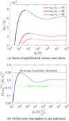Fig. 3. Panel a: series of equilibria of the Brownian population with total mass Mb embedded in a Plummer host cluster with total mass, M⋆, for three different individual mass ratios. The x-axis is the dimensionless density at the center. The presence of a maximum at each curve designates an instability. No equilibrium exists above the maximum at each case, while the dotted curves correspond to equilibria that cannot be supported by inhomogeneous Brownian pressure alone. Panel b: three curves of panel a merge to a single one when scaled properly with the individual mass ratios. The y-axis variable is the Spitzer parameter S. In Brownian inhomogeneous diffusion, equilibria exist above the Spitzer instability threshold SSpitzer = 0.16. The instability sets in at S = 0.25, p̃b(0)(m⋆/mb)3/2 = 140 in the case of a Plummer host cluster.

We further discover numerically that when the BH subcluster mass is scaled to become the Spitzer parameter,

$$\begin{array}{c}\hfill S\equiv \frac{M_{\mathrm{b}}{m}_{\mathrm{b}}^{3/2}}{M_{\star }{m}_{\star }^{3/2}}\end{array}$$(27)

and the central probability density is scaled as

$$\begin{array}{c}\hfill B\equiv {\stackrel{\sim }{p}}_{\mathrm{b}}(0){\left(\frac{m_{\star }}{m_{\mathrm{b}}}\right)}^{3/2},\end{array}$$(28)

then all curves with different ratios, m_b/m_⋆, merge to form a single one, as in Fig. 3b (we estimate the exact value of the exponent to be 1.51 and not 3/2, but we consider this small deviation a numerical precision effect without any physical significance). Thus, the curve Fig. 3b is global and applies to all Brownian populations immersed in a Plummer profile. The instability sets in at

$$\begin{array}{c}\hfill B_{\mathrm{I}}=140,S_{\mathrm{I}}=0.25.\end{array}$$(29)

Any stationary equilibrium with

$$\begin{array}{c}\hfill B>B_{\mathrm{I}}\end{array}$$(30)

is unstable within the current framework. In addition no stationary equilibrium states exist above

$$\begin{array}{c}\hfill S>S_{\mathrm{I}}.\end{array}$$(31)

This value S_I is significantly larger than the Spitzer value (Spitzer 1969), S_SP = 0.16, calculated for isothermal equipartition.

We stress at this point that while we assume here that the BH population to be immersed inside a fixed density profile of the cluster, it should, in practice, affect the cluster profile at least in the vicinity of BH subcluster’s denser regions. This effect, not taken into account in the current work, may influence the cluster’s ability to support the BH population. Nevertheless, it seems possible that the BH population will locally heat up and inflate the population of lighter bodies in an effect that is similar to osmosis. This could possibly enhance, rather than reduce, a cluster’s ability to support the BH population via gravitational fluctuations and could lead to formation of a core (as e.g., proposed by Merritt et al. 2004). Such BH population feedback onto the cluster density profile requires further investigation and is not studied here.

The density profile of a BH population at the onset of the instability appears in Fig. 4, where the Plummer profile, ρ_⋆, is also plotted. It is evident that the BH subcluster may extend up to 0.2 pc inside the host cluster and it may be almost twice as dense in the centre.

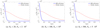Fig. 4. Mass density ρb(r) = Mbpb(r) of a marginally stable BH population given by the solution of the system (25) and (26). The average individual BH mass is assumed to be mb = 10 M⊙ and the Spitzer parameter equals the marginal value of the onset of the instability S = 0.25. The BH population is embedded in a globular cluster with average individual mass density m⋆ = 0.5 M⊙ and half-mass radius rhm = 1 pc. The black dotted line represents the Plummer mass density profile of the host globular cluster.

In Fig. 6, we plot the maximum number of Brownian bodies, that is, BHs, in our context and with respect to their individual average mass for inhomogeneous diffusion and Spitzer instability. We assume m_⋆ = 0.5 M_⊙ and consider two cases of N_⋆ = 10⁶,  10⁸. In the typical case of a globular cluster with N_⋆ = 10⁶ and m_b = 10 M_⊙, for an inhomogeneous diffusion we get N_b ∼ 1400, while the Spitzer threshold is significantly lower at N_b ∼ 890.

In Fig. 7, we compare the probability distribution of a single intermediate-mass BH with BH populations of lighter stellar mass BHs but with equal total mass. It is evident from Fig. 7a that in order to be able to discriminate a BH population from an intermediate-mass BH with a mass of 500m_⋆, it may be required to probe inside the inner 0.1 pc. In Fig. 7b, we show that for a BH population with N_b = 1090, m_b = 10 M_⊙ the first unstable profile is very similar to that of an intermediate-mass BH of equal total mass, while in order to discover observationally the second unstable profile, if stabilized by other processes, one has to probe the inner ∼0.005 pc.

3. Conclusions

In this work, we study inhomogeneous diffusion, that is, diffusion in a medium with varying mass density and temperature and, hence, also varying damping and diffusion coefficients. This is the typical case for self-gravitating systems that are spatially inhomogeneous and trapped in states with varying velocity dispersions. We argue that the inhomogeneous diffusion Eq. (4) applies to self-gravitating systems that involve a sub-population of fewer and heavier bodies and describes gravitational Brownian motion. The corresponding stationary states are given in Eqs. (5) and (6). We calculated the spatial probability distribution function of a single Brownian particle immersed in a Plummer profile, as depicted in Fig. 1. We estimate that a single intermediate-mass BH may wander as far as ∼0.05 pc in a typical Globular cluster, while a single typical stellar BH may wander even ten times farther. We validate the reality of inhomogeneous diffusion of BHs immersed in stellar clusters, expressed by Eq. (1), with the use of N-body simulations, as in Fig. 2. The theoretical prediction is well-matched by the simulation results.

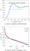Fig. 5. Panel a: series of equilibria of BH populations with individual BH mass, mb = 10 M⊙, expressed by the number of BHs, Nb, with respect to the BH population central density, ρb(0). The BH population is immersed in a Plummer profile of a globular cluster with average individual stellar mass, m⋆ = 0.5 M⊙, number of stars, N⋆ = 106, and half-mass radius, rhm = 1 pc. For a BH subcluster with S >  0.185, corresponding here to Nb >  100, many equilibrium solutions exist. We consider S = 0.2, that is, Nb = 109 and the first three corresponding equilibria A, B, C. Panel b: density profile of the three stationary states A, B, C specified in panel a. Profile A is stable. The equilibria B and C are unstable with respect to Brownian fluctuations, although they may get stabilized by other processes.

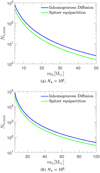Fig. 6. Maximum number of BHs with respect to their individual mass that may maintained at a stationary state inside a Plummer stellar profile with m⋆ = 0.5 M⊙ and two cases of a number of stars of N⋆ = 106,  108. Upper blue curve corresponds to our model for inhomogeneous diffusion, while the lower green one to the Spitzer instability limit derived from the energy equipartition.

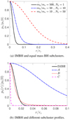Fig. 7. Panel a: probability density distribution of a single massive BH (continuous curve) along with that of BH populations with equal total mass. It is assumed N⋆ = 106. Panel b: a massive BH with mb = 1090 M⊙ (continuous line), along with the three different possible equilibria of Fig. 5 corresponding to the same BH population with Nb = 109, mb = 10 M⊙. It is assumed N⋆ = 106, m⋆ = 0.5 M⊙.

Applying our framework to a Brownian population of massive bodies (focusing on BHs) inside a stellar cluster, which follows a Plummer density profile, we identify an instability that sets in for Brownian populations with Spitzer parameter, S_I = 0.25, and a new global parameter, B_I = 140, which depends on the central density of the Brownian population. This is depicted in Fig. 3. For B >  B_I, any stationary equilibrium state is unstable despite the fluctuations of the gravitational field. For S >  S_I, no stationary states exist. This is a manifestation of the Spitzer instability, reinterpreted as the inability of the cluster to support the sub-population of heavier bodies by gravitational fluctuations. The dependence of the onset of the instability on the individual mass ratios in such a framework arises naturally. Furthermore, since the ordinary Spitzer instability occurs at a lower value, S_SP = 0.16, the inhomogeneous diffusion allows more massive BH populations to reach stationary states than one would expect from isothermal equipartition.

An important limitation of our model for BH populations in Sect. 2.2 regarding its physical applicability is that it does not take into account the feedback of the BH population to the gravitational potential of the host cluster. Such a limitation for analyses on the Brownian motion of a single massive BH was also noted in Merritt et al. (2007). The situation is very similar since our BH population has the same mass of our assumed single massive BH and it turns out to have about the same spatial probability distribution. Still, it was our intention to neglect this feedback in order to quantify the effect solely of the gravitational fluctuations to the BH population and inspect their stabilizing efficiency. If anything, it seems plausible that the BH population will locally heat up and inflate the population of lighter bodies, as was also suggested by Merritt et al. (2004). This will enhance, and not reduce, the cluster’s ability to support the BH population via gravitational fluctuations and lead to the formation of a core. We remark that in his seminal work on Brownian motion, Einstein (1905, 1956) interpreted it precisely as a response to osmotic pressure. Osmosis involves the diffusion of the solvent particles (in our case the stars) in the region of the solute (in our case, the BH population), with result the inflation of the region containing the solute. Such BH population feedback onto the cluster density profile, including the possible reality of such a phenomenon as “gravitational osmosis”, requires further investigation. Another future improvement could include following the time evolution of the diffusion Eq. (4) for the BH population.

In conclusion, the fact that a BH subcluster can be supported by random fluctuations of the gravitational field beyond the limit of Spitzer instability threshold supports the idea that globular clusters can retain a significant BH population.

References

Appendix A: Diffusion equation for gravitational Brownian motion

We reproduce here the diffusion equation of Brownian motion inside an inhomogeneous medium with varying temperature, as was first proposed by van Kampen (1988). We further argue that this diffusion equation describes gravitational Brownian motion. It applies to self-gravitating systems, which are not only inhomogeneous, but also are typically non-isothermal, in the sense that the velocity dispersion varies with position.

As suggested by Chandrasekhar (1943a), the gravitational field, g(r, t), at a point, r, and time, t, of an N-body self-gravitating system may be decomposed to the sum of a mean field g_m and a fluctuating field g_f:

$$\begin{array}{c}\hfill \mathit{g}(\mathit{r},t)={\mathit{g}}_{\mathrm{m}}(\mathit{r},t)+{\mathit{g}}_{\mathrm{f}}(\mathit{r},t).\end{array}$$(A.1)

The mean field represents the effect of the system as a whole to each point of space at any instant of time through the smoothed out continuous mass density function ρ(r, t):

$$\begin{array}{c}\hfill {\mathit{g}}_{\mathrm{m}}=-\mathrm{\nabla }\mathrm{\Phi },\mathrm{\Phi }(\mathit{r},t)=-{\displaystyle \int \mathrm{d}}\stackrel{\sim }{\mathit{r}}G\frac{\rho (\mathit{r},t)}{|\mathit{r}-\stackrel{\sim }{\mathit{r}}|}·\end{array}$$(A.2)

The fluctuating field accounts for the deviations from this smoothed out field that arise due to the granularity of the system. Chandrasekhar (1943b) showed further that each body is subject to a dynamical friction force with a damping coefficient, η, which is reciprocal to the relaxation timescale of the system. Central to his derivation is a Fokker-Planck type of equation discovered by Kramers, namely,

$$\begin{array}{c}\hfill (\frac{\partial }{\partial t}+v\frac{\partial }{\partial x}-{\mathrm{\Phi }}^{\prime }\frac{\partial }{\partial v})f(x,v,t)=\eta \frac{\partial }{\partial v}(v+\frac{T}{m}\frac{\partial }{\partial v})f(x,v,t),\end{array}$$(A.3)

which we consider here in one-dimension for simplicity without loss of generality. We denote f as the phase-space probability distribution function, m the mass of the Brownian particle, T the temperature in units k_B = 1, and η the damping coefficient. Equation (A.3) was derived by Kramers (1940) according to very general considerations. Chandrasekhar (1943a) rederived alternatively Kramers equation and used it in self-gravitating systems to establish the concept of dynamical friction (Chandrasekhar 1943b). Here, following van Kampen (1988), we consider Kramers equation, but with varying damping (dynamical friction in our case) coefficient and temperature,

$$\begin{array}{c}\hfill \eta =\eta (x),T=T(x).\end{array}$$(A.4)

From Eq. (A.3), we derive the diffusion equation, which is to be a generalization of the Smolukowski equation and we argue that it describes gravitational Brownian motion.

First, for the purposes of completeness, we reproduce the derivation of (A.3) following Chandrasekhar (1943a). We assume that the motion of a Brownian particle is described by a Langevin equation,

$$\begin{array}{c}\hfill \frac{\mathrm{d}v}{\mathrm{d}t}=-\eta v+g_{\mathrm{m}}+g_{\mathrm{f}},\end{array}$$(A.5)

where η is the dynamical friction coefficient (Chandrasekhar 1943b), g_m = −Φ′ is the mean field and g_f the fluctuating field. The latter term has statistically defined properties rendering the Langevin equation a stochastic differential equation that cannot be solved as an ordinary differential equation might be. Instead, we would aim to derive a distribution function f(x, v, t + Δt) governing the probability of occurrence of x,v at time t + Δt given the distribution, f(x, v, t), at time, t.

We let Δt be short with respect to the relaxation time Δt ≪ η⁻¹ but long compared to the period of g_f fluctuations. We define the velocity variation due to field fluctuation within Δt,

$$\begin{array}{c}\hfill B(\mathrm{\Delta }t)={\displaystyle {\int }_t^{t+\mathrm{\Delta }t}}{g}_{\mathrm{f}}(\xi )\mathrm{d}\xi .\end{array}$$(A.6)

Physically, it describes the net acceleration exerted on the Brownian particle arising from field fluctuations in time, Δt. We impose the physical requirement that for t → ∞, i.e. t ≫ η⁻¹ that is at zeroth order of η⁻¹, the distribution function, f, is locally Maxwellian. Chandrasekhar (1943a) has proven, as in his Chapter II.2, that this requirement implies that B satisfies the Brownian probability distribution:

$$\begin{array}{c}\hfill \psi (B)={\left(\frac{m}{4\pi \eta T\mathrm{\Delta }t}\right)}^{1/2}{e}^{-\frac{m}{4\eta T\mathrm{\Delta }t}{B}^2}.\end{array}$$(A.7)

The spatial and velocity displacements, Δx, Δv, at Δt are derived by the Langevin Eq. (A.5), so that we get

$$\begin{array}{c}\hfill \mathrm{\Delta }x=v\mathrm{\Delta }t,B=\mathrm{\Delta }v+(\eta v+{\mathrm{\Phi }}^{\prime })\mathrm{\Delta }t.\end{array}$$(A.8)

The latter equation follows by integration of the Langevin Eq. (A.5) from t to t + Δt, introducing B by use of (A.6), and finally solving with respect to B.

Given that Brownian motion is governed by two-body relaxation and it proceeds in a short timescale, it is reasonably expected to be modelled as a Markoff process² In this case the probability distribution at any time, t + Δt, can be derived from the distribution at previous time, t. Using Eq. (A.8), the transition probability, ψ(v − Δv; Δv), that v changes by Δv may be expressed with respect only to Δv. Then we have:

$$\begin{array}{c}\hfill f(x+v\mathrm{\Delta }t,v,t+\mathrm{\Delta }t)=\int \mathrm{d}(\mathrm{\Delta }v)f(x,v-\mathrm{\Delta }v,t)\psi (x,v-\mathrm{\Delta }v;\mathrm{\Delta }v),\end{array}$$(A.9)

where ψ is given from (A.7) for B(Δv) given in (A.8). Taylor expanding f(x + vΔt, v, t + Δt), f(x, v − Δv, t) and ψ(x, v − Δv; Δv) we get the Fokker-Planck equation:

$$\begin{array}{c}\hfill (\frac{\partial f}{\partial t}+v\frac{\partial f}{\partial x})\mathrm{\Delta }t+\mathcal{O}({(\mathrm{\Delta }t)}^2)=-\frac{\partial (f⟨\mathrm{\Delta }v⟩)}{\partial v}+\frac{1}{2}\frac{\partial (f⟨\mathrm{\Delta }{v}^2⟩)}{\partial v^2}+\mathcal{O}({(\mathrm{\Delta }t)}^2),\end{array}$$(A.10)

where the mean values ⟨ • ⟩ are calculated with the distribution ψ(x, v; Δv). We get ⟨Δv⟩ =  − (ηv + Φ′)Δt and ⟨(Δv)²⟩ = (2ηT/m)Δt + 𝒪(Δt²). Making a substitution in (A.10), we get finally Kramers Eq. (A.3), generalized for an inhomogeneous medium:

$$\begin{array}{c}\hfill (\frac{\partial }{\partial t}+v\frac{\partial }{\partial x}-\mathrm{\Phi }{(x)}^{\prime }\frac{\partial }{\partial v})f(x,v,t)=\eta (x)\frac{\partial }{\partial v}(v+\frac{T(x)}{m}\frac{\partial }{\partial v})f(x,v,t).\end{array}$$(A.11)

Now, we derive the corresponding diffusion equation from Kramers equation following van Kampen (1988), who uses a well-established method that was also used to derive the Smolukowski equation from the Kramers equation (Chandrasekhar 1943a), but modified in a straightforward manner to account for the dependence of η and T on x. That is a method of elimination of fast variables (Van Kampen 1985) in which we expand the solution to (A.11) in powers of

$$\begin{array}{c}\hfill \epsilon (x)\equiv \eta {(x)}^{-1},\end{array}$$(A.12)

which is the local relaxation time (Chandrasekhar 1943a). We assume

$$\begin{array}{c}\hfill f=f^{(0)}+f^{(1)}+f^{(2)}+\mathcal{O}({\epsilon }^3)\end{array}$$(A.13)

and get up to the second order the equations

$$\begin{array}{cc}& \frac{\partial }{\partial v}(v{f}^{(0)}+\frac{T}{m}\frac{\partial f^{(0)}}{\partial v})=0\hfill \end{array}$$(A.14)

$$\begin{array}{cc}& \epsilon (\frac{\partial f^{(0)}}{\partial t}+v\frac{\partial f^{(0)}}{\partial x}-{\mathrm{\Phi }}^{\prime }\frac{\partial f^{(0)}}{\partial v})=\frac{\partial }{\partial v}(v{f}^{(1)}+\frac{T}{m}\frac{\partial f^{(1)}}{\partial v})\hfill \end{array}$$(A.15)

$$\begin{array}{cc}& \epsilon (\frac{\partial f^{(1)}}{\partial t}+v\frac{\partial f^{(1)}}{\partial x}-{\mathrm{\Phi }}^{\prime }\frac{\partial f^{(1)}}{\partial v})=\frac{\partial }{\partial v}(v{f}^{(2)}+\frac{T}{m}\frac{\partial f^{(2)}}{\partial v})·\hfill \end{array}$$(A.16)

Requiring that f⁽⁰⁾ vanishes for |v| → ∞, the first equation gives

$$\begin{array}{c}\hfill f^{(0)}=s(x,t)e^{-\frac{m{v}^2}{2T(x)}},\end{array}$$(A.17)

for some function, s(x, t), to be determined. The integral of the right-hand side of Eq. (A.15) is zero:

$$\begin{array}{c}\hfill {\displaystyle {\int }_{-\infty }^{+\infty }}\mathrm{d}v(v{f}^{(1)}+\frac{T}{m}\frac{\partial f^{(1)}}{\partial v})=0\end{array}$$(A.18)

and therefore the integral on the left-hand side should also be zero:

$$\begin{array}{c}\hfill {\displaystyle {\int }_{-\infty }^{+\infty }}\mathrm{d}v\frac{\partial f^{(0)}}{\partial t}+{\displaystyle {\int }_{-\infty }^{+\infty }}\mathrm{d}vv\frac{\partial f^{(0)}}{\partial x}-{\displaystyle {\int }_{-\infty }^{+\infty }}\mathrm{d}v{\mathrm{\Phi }}^{\prime }\frac{\partial f^{(0)}}{\partial v}=0\end{array}$$(A.19)

Substituting Eq. (A.17) we have

$$\begin{array}{cc}& {\displaystyle {\int }_{-\infty }^{+\infty }}\mathrm{d}vv\frac{\partial f^{(0)}}{\partial x}=s^{\prime }{\displaystyle {\int }_{-\infty }^{+\infty }}\mathrm{d}vv{e}^{-\frac{m{v}^2}{2T}}+s\frac{m{T}^{\prime }}{2T^2}{\displaystyle {\int }_{-\infty }^{+\infty }}\mathrm{d}v{v}^3{e}^{-\frac{m{v}^2}{2T}}=0\hfill \\ \hfill & {\displaystyle {\int }_{-\infty }^{+\infty }}\mathrm{d}v{\mathrm{\Phi }}^{\prime }\frac{\partial f^{(0)}}{\partial v}=s{\mathrm{\Phi }}^{\prime }{\displaystyle {\int }_{-\infty }^{+\infty }}\mathrm{d}v\frac{\partial }{\mathrm{d}v}\left(e^{-\frac{m{v}^2}{2T}}\right)=0\hfill \end{array}$$

and therefore Eq. (A.19) gives the integrability condition:

$$\begin{array}{c}\hfill \frac{\partial f^{(0)}}{\partial t}=0,\end{array}$$(A.20)

which results finally in

$$\begin{array}{c}\hfill f^{(0)}=f^{(0)}(x,v)=s(x)e^{-\frac{m{v}^2}{2T(x)}}.\end{array}$$(A.21)

We substitute this in Eq. (A.15) and get

$$\begin{array}{cc}\hfill \epsilon e^{-\frac{m{v}^2}{2T}}(v{s}^{\prime }+\frac{v}{T}m{\mathrm{\Phi }}^{\prime }s+\frac{v^3}{2T^2}m{T}^{\prime }s)& =\frac{\partial }{\partial v}(v{f}^{(1)}+\frac{T}{m}\frac{\partial f^{(1)}}{\partial v})\hfill \\ \hfill & =\frac{T}{m}\frac{\partial }{\partial v}\left(e^{-\frac{m{v}^2}{2T}}\frac{\partial }{\partial v}{e}^{\frac{m{v}^2}{2T}}{f}^{(1)}\right).\hfill \end{array}$$(A.22)

The ansatz

$$\begin{array}{c}\hfill f^{(1)}(x,v,t)=(vh(x,t)+v^{3}q(x,t))e^{-\frac{m{v}^2}{2T}}\end{array}$$(A.23)

gives

$$\begin{array}{cc}& h=h(x)=-\frac{{(T(x)s(x))}^{\prime }+m\mathrm{\Phi }{(x)}^{\prime }s(x)}{T(x)}\epsilon (x)\hfill \end{array}$$(A.24)

$$\begin{array}{cc}& q=q(x)=-\frac{mT{(x)}^{\prime }}{6T{(x)}^2}\epsilon (x)s(x).\hfill \end{array}$$(A.25)

Both h and q do not depend on time. The general solution may be obtained by adding a solution of the homogeneous problem

$$\begin{array}{c}\hfill f^{(1)}(x,v,t)=\epsilon (-v\frac{T^{\prime }}{T}s-v{s}^{\prime }-v\frac{m{\mathrm{\Phi }}^{\prime }}{T}s-v^3\frac{m{T}^{\prime }}{6T^2}s+w(t))e^{-\frac{m{v}^2}{2T}},\end{array}$$(A.26)

where ε, T, Φ, s depend only on x. We have

$$\begin{array}{c}\hfill p(x,t)\equiv {\displaystyle {\int }_{-\infty }^{+\infty }}\mathrm{d}vf(x,v,t)=\sqrt{2\pi \frac{T(x)}{m}}(s(x)+\epsilon (x)w(t))+\mathcal{O}({\epsilon }^2),\end{array}$$(A.27)

where p is the probability density in space. For N Brownian particles, n = Np can be identified as their average number density.

Equation (A.16) gives the integrability condition

$$\begin{array}{c}\hfill {\displaystyle {\int }_{-\infty }^{+\infty }}\mathrm{d}v\frac{\partial f^{(1)}}{\partial t}=-\frac{\partial }{\partial x}{\displaystyle {\int }_{-\infty }^{+\infty }}\mathrm{d}vv{f}^{(1)}.\end{array}$$(A.28)

Since ∂f⁽⁰⁾/∂t = 0, we have

$$\begin{array}{cc}\hfill \frac{\partial p(x,t)}{\partial t}& =-\frac{\partial }{\partial x}{\displaystyle {\int }_{-\infty }^{+\infty }}\mathrm{d}vv{f}^{(1)}+\mathcal{O}({\epsilon }^2)\hfill \\ \hfill & =\frac{\partial }{\partial x}\left\{\epsilon (\frac{\partial }{\partial x}\left(\frac{T}{m}\sqrt{2\pi \frac{T}{m}}(s+\epsilon w)\right)+{\mathrm{\Phi }}^{\prime }\sqrt{2\pi \frac{T}{m}}(s+\epsilon w))\right\}\hfill \\ \hfill & +\mathcal{O}({\epsilon }^2),\hfill \end{array}$$(A.29)

which gives, by substitution of (A.27), to first order in ε, the diffusion equation

$$\begin{array}{c}\hfill \frac{\partial p(x,t)}{\partial t}=\frac{\partial }{\partial x}\left\{\mu (x)(m\mathrm{\Phi }{(x)}^{\prime }p(x,t)+\frac{\partial }{\partial x}(T(x)p(x,t)))\right\},\end{array}$$(A.30)

where we denote μ(x) = ε(x)/m = 1/mη(x). This is the Van Kampen inhomogeneous diffusion equation that we suggest applies to gravitational Brownian motion.

All Figures

Fig. 1. Stationary probability distribution pb of inhomogeneous diffusion (5) with respect to distance, r, for a single Brownian body, mb, inside a Plummer external gravitational potential. The Brownian body may be considered to be a massive BH and the gravitational potential may be generated by a globular cluster of individual average stellar mass, m⋆. We denote rc the softening radius of the potential.

In the text

Fig. 2. N-body simulations with AMUSE framework of a BH with mass mb = 50 M⊙ immersed with zero velocity in the center, rb, ini = 1 AU, of a stellar cluster with N⋆ = 1000, m⋆ = 0.5 M⊙, and initial conditions sampled from a Plummer sphere with softening radius, rc = 0.5 pc. (a) Radial position of the BH with respect to time in a single run. (b) Probability density of the position of the BH for 1000 runs. See text for details.

In the text

Fig. 3. Panel a: series of equilibria of the Brownian population with total mass Mb embedded in a Plummer host cluster with total mass, M⋆, for three different individual mass ratios. The x-axis is the dimensionless density at the center. The presence of a maximum at each curve designates an instability. No equilibrium exists above the maximum at each case, while the dotted curves correspond to equilibria that cannot be supported by inhomogeneous Brownian pressure alone. Panel b: three curves of panel a merge to a single one when scaled properly with the individual mass ratios. The y-axis variable is the Spitzer parameter S. In Brownian inhomogeneous diffusion, equilibria exist above the Spitzer instability threshold SSpitzer = 0.16. The instability sets in at S = 0.25, p̃b(0)(m⋆/mb)3/2 = 140 in the case of a Plummer host cluster.

In the text

Fig. 4. Mass density ρb(r) = Mbpb(r) of a marginally stable BH population given by the solution of the system (25) and (26). The average individual BH mass is assumed to be mb = 10 M⊙ and the Spitzer parameter equals the marginal value of the onset of the instability S = 0.25. The BH population is embedded in a globular cluster with average individual mass density m⋆ = 0.5 M⊙ and half-mass radius rhm = 1 pc. The black dotted line represents the Plummer mass density profile of the host globular cluster.

In the text

Fig. 5. Panel a: series of equilibria of BH populations with individual BH mass, mb = 10 M⊙, expressed by the number of BHs, Nb, with respect to the BH population central density, ρb(0). The BH population is immersed in a Plummer profile of a globular cluster with average individual stellar mass, m⋆ = 0.5 M⊙, number of stars, N⋆ = 106, and half-mass radius, rhm = 1 pc. For a BH subcluster with S >  0.185, corresponding here to Nb >  100, many equilibrium solutions exist. We consider S = 0.2, that is, Nb = 109 and the first three corresponding equilibria A, B, C. Panel b: density profile of the three stationary states A, B, C specified in panel a. Profile A is stable. The equilibria B and C are unstable with respect to Brownian fluctuations, although they may get stabilized by other processes.

In the text

	Fig. 6. Maximum number of BHs with respect to their individual mass that may maintained at a stationary state inside a Plummer stellar profile with m⋆ = 0.5 M⊙ and two cases of a number of stars of N⋆ = 106,  108. Upper blue curve corresponds to our model for inhomogeneous diffusion, while the lower green one to the Spitzer instability limit derived from the energy equipartition.
In the text

	Fig. 7. Panel a: probability density distribution of a single massive BH (continuous curve) along with that of BH populations with equal total mass. It is assumed N⋆ = 106. Panel b: a massive BH with mb = 1090 M⊙ (continuous line), along with the three different possible equilibria of Fig. 5 corresponding to the same BH population with Nb = 109, mb = 10 M⊙. It is assumed N⋆ = 106, m⋆ = 0.5 M⊙.
In the text

References

- Abbate, F., Possenti, A., Colpi, M., & Spera, M. 2019, ApJ, 884, L9 [NASA ADS] [CrossRef] [Google Scholar]
- Arca-Sedda, M. 2016, MNRAS, 455, 35 [NASA ADS] [CrossRef] [Google Scholar]
- Arca Sedda, M., Askar, A., & Giersz, M. 2018, MNRAS, 479, 4652 [NASA ADS] [CrossRef] [Google Scholar]
- Askar, A., Arca Sedda, M., & Giersz, M. 2018, MNRAS, 478, 1844 [NASA ADS] [CrossRef] [Google Scholar]
- Bahramian, A., Heinke, C. O., Tudor, V., et al. 2017, MNRAS, 467, 2199 [NASA ADS] [CrossRef] [Google Scholar]
- Barnard, R., Stiele, H., Hatzidimitriou, D., et al. 2008, ApJ, 689, 1215 [NASA ADS] [CrossRef] [Google Scholar]
- Binney, J., & Lacey, C. 1988, MNRAS, 230, 597 [NASA ADS] [CrossRef] [Google Scholar]
- Binney, J., & Tremaine, S. 2008, Galactic Dynamics: Second Edition (Princeton: Princeton University Press) [Google Scholar]
- Bortolas, E., Gualandris, A., Dotti, M., Spera, M., & Mapelli, M. 2016, MNRAS, 461, 1023 [NASA ADS] [CrossRef] [Google Scholar]
- Breen, P. G., & Heggie, D. C. 2013, MNRAS, 432, 2779 [NASA ADS] [CrossRef] [Google Scholar]
- Chandrasekhar, S. 1943a, Rev. Mod. Phys., 15, 1 [NASA ADS] [CrossRef] [Google Scholar]
- Chandrasekhar, S. 1943b, ApJ, 97, 255 [NASA ADS] [CrossRef] [Google Scholar]
- Chatterjee, P., Hernquist, L., & Loeb, A. 2002a, ApJ, 572, 371 [NASA ADS] [CrossRef] [Google Scholar]
- Chatterjee, P., Hernquist, L., & Loeb, A. 2002b, Phys. Rev. Lett., 88, 121103 [CrossRef] [Google Scholar]
- Chatterjee, P., Hernquist, L., & Loeb, A. 2003, ApJ, 592, 32 [CrossRef] [Google Scholar]
- Chatterjee, S., Rodriguez, C. L., & Rasio, F. A. 2017, ApJ, 834, 68 [NASA ADS] [CrossRef] [Google Scholar]
- Chavanis, P.-H. 2012, Phys. A: Stat. Mech. Appl., 391, 3680 [NASA ADS] [CrossRef] [MathSciNet] [Google Scholar]
- Chavanis, P. H. 2013, A&A, 556, A93 [NASA ADS] [CrossRef] [EDP Sciences] [Google Scholar]
- Chomiuk, L., Strader, J., Maccarone, T. J., et al. 2013, ApJ, 777, 69 [NASA ADS] [CrossRef] [Google Scholar]
- Di Cintio, P., Ciotti, L., & Nipoti, C. 2020, IAU Symposium, 351, 93 [Google Scholar]
- Einstein, A. 1905, Annal. Phys., 322, 549 [NASA ADS] [CrossRef] [Google Scholar]
- Einstein, A. 1956, Investigations on the theory of Brownian movement (Dover Publications, Inc.) [Google Scholar]
- El-Zant, A. A., Freundlich, J., & Combes, F. 2016, MNRAS, 461, 1745 [Google Scholar]
- El-Zant, A. A., Freundlich, J., Combes, F., & Halle, A. 2020, MNRAS, 492, 877 [CrossRef] [Google Scholar]
- Fouvry, J.-B., & Bar-Or, B. 2018, MNRAS, 481, 4566 [CrossRef] [Google Scholar]
- Giesers, B., Dreizler, S., Husser, T.-O., et al. 2018, MNRAS, 475, L15 [NASA ADS] [CrossRef] [Google Scholar]
- Heggie, D., & Hut, P. 2003, The Gravitational Million-Body Problem: A Multidisciplinary Approach to Star Cluster Dynamics (Cambridge: Cambridge University Press) [CrossRef] [Google Scholar]
- Irwin, J. A., Brink, T. G., Bregman, J. N., & Roberts, T. P. 2010, ApJ, 712, L1 [NASA ADS] [CrossRef] [Google Scholar]
- Kramers, H. A. 1940, Physica, 7, 284 [NASA ADS] [CrossRef] [MathSciNet] [Google Scholar]
- Kremer, K., Ye, C. S., Chatterjee, S., Rodriguez, C. L., & Rasio, F. A. 2018, ApJ, 855, L15 [NASA ADS] [CrossRef] [Google Scholar]
- Kremer, K., Chatterjee, S., Ye, C. S., Rodriguez, C. L., & Rasio, F. A. 2019, ApJ, 871, 38 [CrossRef] [Google Scholar]
- Kulkarni, S. R., Hut, P., & McMillan, S. 1993, Nature, 364, 421 [NASA ADS] [CrossRef] [Google Scholar]
- Lau, J. Y., & Binney, J. 2019, MNRAS, 490, 478 [CrossRef] [Google Scholar]
- Lingam, M. 2018, MNRAS, 473, 1719 [CrossRef] [Google Scholar]
- Maccarone, T. J., Kundu, A., Zepf, S. E., & Rhode, K. L. 2007, Nature, 445, 183 [NASA ADS] [CrossRef] [PubMed] [Google Scholar]
- Mackey, A. D., Wilkinson, M. I., Davies, M. B., & Gilmore, G. F. 2008, MNRAS, 386, 65 [NASA ADS] [CrossRef] [Google Scholar]
- Merritt, D. 2005, ApJ, 628, 673 [CrossRef] [Google Scholar]
- Merritt, D. 2013, Dynamics and Evolution of Galactic Nuclei (Princeton: Princeton University Press) [Google Scholar]
- Merritt, D., Piatek, S., Portegies Zwart, S., & Hemsendorf, M. 2004, ApJ, 608, L25 [NASA ADS] [CrossRef] [Google Scholar]
- Merritt, D., Berczik, P., & Laun, F. 2007, AJ, 133, 553 [NASA ADS] [CrossRef] [Google Scholar]
- Miller-Jones, J. C. A., Strader, J., Heinke, C. O., et al. 2015, MNRAS, 453, 3918 [CrossRef] [Google Scholar]
- Minniti, D., Contreras Ramos, R., Alonso-García, J., et al. 2015, ApJ, 810, L20 [NASA ADS] [CrossRef] [Google Scholar]
- Morscher, M., Umbreit, S., Farr, W. M., & Rasio, F. A. 2013, ApJ, 763, L15 [NASA ADS] [CrossRef] [Google Scholar]
- Morscher, M., Pattabiraman, B., Rodriguez, C., Rasio, F. A., & Umbreit, S. 2015, ApJ, 800, 9 [NASA ADS] [CrossRef] [Google Scholar]
- Pelupessy, F. I., van Elteren, A., de Vries, N., et al. 2013, A&A, 557, A84 [NASA ADS] [CrossRef] [EDP Sciences] [Google Scholar]
- Portegies Zwart, S., & McMillan, S. 2018, Astrophysical Recipes, 2514-3433 (IOP Publishing) [Google Scholar]
- Portegies Zwart, S., McMillan, S., Harfst, S., et al. 2009, New Astron., 14, 369 [NASA ADS] [CrossRef] [Google Scholar]
- Portegies Zwart, S., McMillan, S. L. W., van Elteren, E., Pelupessy, I., & de Vries, N. 2013, Comput. Phys. Commun., 184, 456 [NASA ADS] [CrossRef] [Google Scholar]
- Rauch, K. P., & Tremaine, S. 1996, New Astron., 1, 149 [NASA ADS] [CrossRef] [Google Scholar]
- Roberts, T. P., Fabbiano, G., Luo, B., et al. 2012, ApJ, 760, 135 [CrossRef] [Google Scholar]
- Rodriguez, C. L., Morscher, M., Wang, L., et al. 2016, MNRAS, 463, 2109 [NASA ADS] [CrossRef] [Google Scholar]
- Roupas, Z. 2020, J. Phys. A Math. Gen., 53, 045002 [CrossRef] [Google Scholar]
- Roupas, Z., Kocsis, B., & Tremaine, S. 2017, ApJ, 842, 90 [NASA ADS] [CrossRef] [Google Scholar]
- Shishkovsky, L., Strader, J., Chomiuk, L., et al. 2018, ApJ, 855, 55 [NASA ADS] [CrossRef] [Google Scholar]
- Sigurdsson, S., & Hernquist, L. 1993, Nature, 364, 423 [NASA ADS] [CrossRef] [Google Scholar]
- Spitzer, L., Jr. 1969, ApJ, 158, L139 [NASA ADS] [CrossRef] [Google Scholar]
- Strader, J., Chomiuk, L., Maccarone, T. J., Miller-Jones, J. C. A., & Seth, A. C. 2012, Nature, 490, 71 [NASA ADS] [CrossRef] [Google Scholar]
- Taylor, M. A., Puzia, T. H., Gomez, M., & Woodley, K. A. 2015, ApJ, 805, 65 [NASA ADS] [CrossRef] [Google Scholar]
- Tremaine, S. 2020, MNRAS, 493, 2632 [CrossRef] [Google Scholar]
- Tremaine, S., & Weinberg, M. D. 1984, MNRAS, 209, 729 [NASA ADS] [CrossRef] [Google Scholar]
- Van Kampen, N. G. 1985, Phys. Rep., 124, 69 [CrossRef] [MathSciNet] [Google Scholar]
- van Kampen, N. 1988, J. Phys. Chem. Solids, 49, 673 [CrossRef] [Google Scholar]
- Vasiliev, E. 2017, ApJ, 848, 10 [CrossRef] [Google Scholar]
- Wang, L., Spurzem, R., Aarseth, S., et al. 2016, MNRAS, 458, 1450 [NASA ADS] [CrossRef] [Google Scholar]
- Weatherford, N. C., Chatterjee, S., Rodriguez, C. L., & Rasio, F. A. 2018, ApJ, 864, 13 [NASA ADS] [CrossRef] [Google Scholar]
- Weatherford, N. C., Chatterjee, S., Kremer, K., & Rasio, F. A. 2019, ApJ, 898, 162 [Google Scholar]