| Issue |
A&A
Volume 646, February 2021
|
|
|---|---|---|
| Article Number | A154 | |
| Number of page(s) | 9 | |
| Section | Astrophysical processes | |
| DOI | https://doi.org/10.1051/0004-6361/202038621 | |
| Published online | 19 February 2021 | |
A variable magnetic disc wind in the black hole X-ray binary GRS 1915+105?
1
Department of Physics, Tor Vergata University of Rome, Via della Ricerca Scientifica 1, 00133 Rome, Italy
e-mail: This email address is being protected from spambots. You need JavaScript enabled to view it.
2
INAF – IAPS, Via Fosso del Cavaliere 100, 00133 Rome, Italy
3
INAF – Astronomical Observatory of Rome, Via Frascati 33, 00078 Monte Porzio Catone (Rome), Italy
4
INFN – Tor Vergata, Via della Ricerca Scientifica 1, 00133 Rome, Italy
5
Department of Astronomy, University of Maryland, College Park, MD 20742, USA
6
NASA/Goddard Space Flight Center, Greenbelt, MD 20771, USA
7
James Madison University, 800 South Main Street, Harrisonburg, VA 22807, USA
Received:
9
June
2020
Accepted:
14
December
2020
Abstract
Context. GRS 1915+105 being one of the brightest transient black hole binaries (BHBs) in the X-rays offers a unique testbed for the study of the connection between accretion and ejection mechanisms in BHBs. In particular, this source can be used to study the accretion disc wind and its dependence on the state changes in BHBs.
Aims. Our aim is to investigate the origin and geometry of the accretion disc wind in GRS 1915+105. This study will provide a basis for planning future observations with the X-ray Imaging Spectroscopy Mission (XRISM), and may also provide important parameters for estimating the polarimetric signal with the upcoming Imaging X-ray Polarimetry Explorer (IXPE).
Methods. We analysed the spectra of GRS 1915+105 in the soft ϕ and hard χ classes using the high-resolution spectroscopy offered by Chandra HETGS. In the soft state, we find a series of wind absorption lines that follow a non-linear dependence of velocity width, velocity shift, and equivalent width with respect to ionisation, indicating a multiple component or stratified outflow. In the hard state we find only a faint Fe XXVI absorption line. We model the absorption lines in both the states using a dedicated magneto-hydrodynamic (MHD) wind model to investigate a magnetic origin of the wind and to probe the cause of variability in the observed line flux between the two states.
Conclusions. The MHD disc wind model provides a good fit for both states, indicating the possibility of a magnetic origin of the wind. The multiple ionisation components of the wind are well characterised as a stratification of the same magnetic outflow. We find that the observed variability in the line flux between soft and hard states cannot be explained by photo-ionisation alone but is most likely due to a large (three orders of magnitude) increase in the wind density. We find the mass outflow rate of the wind to be comparable to the accretion rate, suggesting an intimate link between accretion and ejection processes that lead to state changes in BHBs.
Key words: accretion, accretion disks / stars: winds, outflows / magnetohydrodynamics (MHD) / X-rays: binaries
© ESO 2021
1. Introduction
Black hole binaries (BHBs) are the best candidates with which to study the connection between accretion and ejection mechanisms because of their high variability and high X-ray flux. The timescale of variability is comparable to human timescales and therefore the whole cycle of accretion and ejection can be studied for a single system. Even though BHBs can be seen as a scaled-down version of active galactic nuclei (AGNs), their observational signatures may partially differ because of the different sources of accreting material, that is, the companion star or galactic gas, respectively, and also the radiation field that is predominantly governed by X-rays.
The variability of low-mass X-ray binaries (LMXBs) can be classified using the hardness intensity diagram (HID) in X-rays as many of them exhibit a hysteresis loop within this diagram (Belloni et al. 2000). Different points in the loop can be attributed to different accretion–ejection geometries. The presence of a powerful jet is generally seen when the source transits from a hard to a soft state (Fender et al. 2004), establishing the connection between BHB states and the launch of the jet. However, GRS 1915+105, although a LMXB, does not exhibit a hysteresis loop in its HID, and was in a comparatively soft state until recently when it became harder in spectra and fainter in brightness (Miller et al. 2019). Outflows in the form of accretion-disc winds have also been seen in several LMXBs (Lee et al. 2002; Miller et al. 2004, 2006b; Miller 2006), mainly but not necessarily in the soft state (Neilsen & Lee 2009). Despite its clear detection, there is no consensus yet on how and where the wind is launched from the accretion disc, and how it affects the state transitions and the launching of the jet. In GRS 1915+105, it was seen that during the states in which the wind was present, the jet was either weak or absent, and during the states in which the wind was absent, the jet was present (Neilsen & Lee 2009). Therefore, understanding the launching mechanism of the wind is required to study the interplay between the wind, the jet, and the accretion states of BHBs, and insight into the launching mechanism, and estimates of the launching site of the wind and the wind mass flux, could help in determining the unknown parameters of the state transitions in X-ray binaries.
The mechanisms responsible for the launching of disc winds are still debated. Current hypotheses can be divided into three groups: (i) thermally driven, (ii) radiation-pressure driven, and (iii) magnetically driven. Evidence has been found for all three processes (Begelman et al. 1983; Ueda et al. 2004; Neilsen 2013; Díaz Trigo & Boirin 2016; Neilsen et al. 2016; Done et al. 2018; Fukumura et al. 2017; Miller et al. 2006a), as well as two component winds where two different mechanisms co-exist, namely magneto-hydrodynamic (MHD) and thermal (Neilsen & Homan 2012). Thermally driven winds are launched when the X-rays near the compact object heat the disc surface to the Compton temperature (TC) (Begelman et al. 1983; Tombesi et al. 2010). The wind is launched at a radius where the plasma thermal velocity is greater than the local escape velocity. However, thermal winds are also possible from 0.1 RC (Woods et al. 1996), where RC is the Compton radius. Radiation-pressure-driven winds are due to the line pressure exerted on partially ionised elements (Castor et al. 1975). Disc winds can also be accelerated by the disc vertical magnetic pressure gradients or by the disc centrifugal forces in combination with magnetic fields (Fukumura et al. 2010, 2017; Blandford & Payne 1982; Contopoulos 1994, 1995; Ferreira 1997). There is also evidence suggesting that disc winds in BHBs are preferentially seen with equatorial geometry (Ponti et al. 2012). During the last decade, significant improvement has been made in modelling accretion disc winds in BHBs using photo-ionisation codes. GRS 1915+105, GRO 1655-40, 4U 1630-47, and H 1743-322 are some of the BHBs that show the presence of disc winds as seen in terms of intense absorption lines in their X-ray spectra (Miller et al. 2015, 2016, 2006a, 2008; Kallman et al. 2009; Neilsen & Homan 2012; Ueda et al. 2009). Several photo-ionisation modellings of these sources point towards a multiple-component outflow or a MHD origin for the wind (Miller et al. 2006a, 2008, 2015, 2016; Kallman et al. 2009). However, there is a paucity of detailed MHD models that can explain the wind origin by directly fitting the data, with Fukumura et al. (2017) in the case of GRO J1655-40 being one of the few examples.
In the case of GRO J1655-40, Miller et al. (2006a) and Kallman et al. (2009) using photo-ionisation modelling, argue that the wind cannot be explained with one component of absorption in the soft state. They estimated the launch radius from the ionisation parameter (ξ) and compared with the Compton radius (RC), disfavouring the possibility of a single-component thermal origin. Kallman et al. (2009) found that the lines with lower blueshift and larger launching radius from the black hole may be consistent with a thermal wind, while Fe K lines with a shorter launching radius and higher blueshift favour a magnetic origin. Neilsen & Homan (2012) made a comparison of the wind in the soft and hard states of GRO 1655-40, and found that photoionisation alone cannot explain the disappearance of many of the absorption lines in the hard state. Neilsen & Homan (2012) further argue for the presence of a hybrid wind (thermal and MHD) in the hard state evolving into a two-component wind in the soft state, as suggested also by Kallman et al. (2009) and Miller et al. (2006a). However, Fukumura et al. (2017), using a physically self-consistent photo-ionised MHD wind model, found that the two components identified by previous works may be well described by a single MHD wind launched from a large range of radii from the accretion disc. Miller et al. (2015, 2016) showed, from a purely photo-ionisation point of view, that at least two or three absorption components were required to model the lines in the case of all of the above-mentioned sources. Another argument disfavouring a thermal origin is the consistency of the launch radius estimated from re-emission of the wind and the ionisation parameter (Trueba et al. 2019; Miller et al. 2015).
From the recent NICER observations of GRS 1915+105, Neilsen et al. (2018) found that the accretion disc wind is persistent, with absorption line flux changing depending on the state and count rate. In the present work, we model the absorption lines in GRS 1915+105 in the two representative soft and hard states using the same MHD model as in the case of Fukumura et al. (2017). We also explore a similar approach as in Ueda et al. (2009), dividing the soft state observation into two epochs where there was an increase in flux. In Sect. 2 we describe the observations and data reductions. In Sect. 3 we show the light curve and the spectra of both soft and hard states. In Sect. 5 we show the phenomenological scaling relations and MHD wind modelling, and finally in Sect. 6 we discuss the results with comparison to previous works.
2. Observations and data reduction
We considered the high-resolution X-ray spectroscopy offered by Chandra High Energy Transmission Gratings Spectrometer (HETGS) data to study the wind variability in different states of GRS 1915+105. The source was observed 22 times by Chandra using the HETGS instrument. However, we decided to analyse two observations, based on the presence and absence of a strong wind as reported in Neilsen & Lee (2009). As GRS 1915+105 does not have a regular hard state as in the case of other black hole X-ray binaries, we distinguished soft and hard states using the spectral class (Φ for soft and χ for hard) as reported in Neilsen & Lee (2009). We limit our analysis to only two observations because the aim of this study is to understand the change in state with respect to the change in wind, for which these two observations form an adequate sample. The two observations are comparatively less affected by pile up and provide a view of the source in two different spectral states. The observation performed on 2007-08-14 with an exposure of 49 ks (obsid:7485) corresponds to a soft state and the one performed on 2000-04-24 with an exposure of 30.3 ks (obsid:660) corresponds to a hard state. Other than being in two spectral states, the observations also differ in the strength and number of emission and absorption lines present in the spectra (Neilsen & Lee 2009). Both observations were in ‘pointing’ mode and ‘timed’ readout mode. We collected the archival data of these observations from the Chandra Data Archive (CDA) and used the CIAO 4.11 software package for the data reduction and analysis (Fruscione et al. 2006). We reprocessed the data using the ‘chandra_repo’ script to ensure data reduction using the latest calibration data base (CALDB 4.8.2). In bright sources, the zeroth-order position cannot be rightly identified by ‘tgdetect’ ‘because of the hole in the zeroth order. Hence the zeroth order was identified by ‘tg_findzo’ as suggested by ‘tgdetect2’. For obsid:660, ACIS S-2 and ACIS S-3 were used to extract the signal, while for obsid:7485, ACIS S-1, ACIS S-2, ACIS S-3, and ACIS S-4 were used. We used only the High Energy Gratings (HEG) spectrum, as it has two-times better energy resolution than the Medium Energy Gratings (MEG) at higher energies. Moreover, we were not interested in the energy range below 1.5 keV as GRS 1915+105 is heavily absorbed in that range and lower energies are more affected by pileup. We examined the +1 and −1 grating spectra separately to check for correspondence before combining them using ‘add_grating_orders’. Finally, we used ‘mkgrmf’ and ‘mkgarf’ to generate the combined rmf and arf response files.
3. Light curve
The light curves for both observations were extracted using the ‘dmextract’ tool. We considered the energy range from 1.5 keV to 7.2 keV. The light curves were analysed and re-binned using ‘lcurve’ of XRONOS 5.22. Figures 1 and 2 show the light curves for both the soft and hard states, respectively. Based on the light curve and colour–colour diagrams, Belloni et al. (2000) classified GRS 1915+105 into 12 classes. Belloni et al. (2000) found that all the classes can be reduced to three fundamental states (A, B, and C). In state B, the accretion disc extends all the way down to the innermost stable circular orbit (ISCO), and in state C the inner accretion disc is not visible for reasons that are still debated. State A corresponds to a soft state with higher soft colour and higher count rate. In obsid:7485, there was an increase in flux observed during the observation. During the initial phase of this observation, the source was in class ϕ (only state A) and in the later phase, the flux of the source increased to that of δ (transition between state A and state B). However, there is no change in the colour–colour diagram indicating it to be in bright ϕ class (Ueda et al. 2009). During obsid:660 the source was in χ class (only state C).
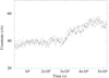 |
Fig. 1. Light curve of GRS1915+105 in the soft state (obsid:7485) with a bin size of 100s. |
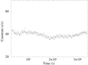 |
Fig. 2. Light curve of GRS1915+105 in the hard state with a bin size of 100s (obsid:660). |
4. Spectral analysis
The combined grating spectra of the first order were analysed using XSPEC 12.10.1. We used only HEG as the energy interval of interest is in the harder X-rays. We find an excess in soft X-rays below 2 keV in both the soft- and hard-state observations peaking at ∼0.12 keV for which the origin might not be physical and might be an instrumental feature. A similar feature for this source is also reported in an XMM-Newton observation reported by Martocchia et al. (2006). We fitted the continuum spectra with a disc black body for the disc emission (diskbb: Mitsuda et al. 1984; Makishima et al. 1986), a black body for the soft excess (bbody), and a power-law continuum for the X-ray corona (nthcomp: Zdziarski et al. 1996; Życki et al. 1999), along with a neutral galactic absorption model (tbabs: Wilms et al. 2000). However, since the spectra are piled up due to the high flux of GRS 1915+105, the parameters of the continuum model should only be considered as a phenomenological best fit. Absorption and emission lines were modelled with a Gaussian (zgauss). Therefore, we concentrate our spectral analysis on the line properties, considering a phenomenological model for the continuum. The χ2 statistic was used for the fit and the errors are calculated at 1σ level. The modelled continuum parameters of all the observations are given in Table 1.
Continuum parameters obtained for the spectral fit for the soft (obsID:7485) and hard (obsID:660) state Chandra observations of GRS 1915+105.
4.1. Soft state
During obsid:7485, GRS 1915+105 was in class ϕ, indicating a relatively soft spectrum dominated by the disc emission. Figure 3 shows the spectrum during the entire observation of 7485 and Fig. 4 shows the zoomed-in version of the same at different energy ranges. We clearly find 20 absorption lines and 1 emission line in the spectrum. The lines were selected based on a minimum threshold of Δχ2 of 15. We fitted the absorption lines with inverted Gaussians and the emission line with a Gaussian. The line at 6.69 keV has previously been shown to split into two in the third-order spectra (Miller et al. 2016). Considering the above case, a double Gaussian was used to model the Fe XXV and Fe XXIV features, as these lines are close enough to overlap into a single observed line within the energy resolution of Chandra HETG first order. The energies of both the Fe XXV and FeXXIV lines were tied to each other by an energy shift of 19.2 eV, and leaving the norm and sigma free to vary. The χ2 value of the best fit is 2928.24 for 2581 degrees of freedom (d.o.f.). There is a wide range of ionic species detected in the spectrum, the dominant ones being Al, Fe, Si, S, Ar, Ca, Cr, Mn, and Fe. The parameters of the detected lines are given in Table 2.
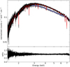 |
Fig. 3. Spectrum of GRS 1915+105 after modelling the absorption and emission lines using the phenomenological Gaussian line profiles. Top panel: spectrum of GRS 1915+105 in the soft state (obsid: 7485) and hard state (obsid: 660). The data in soft and hard states are plotted in black and grey, while the respective models are shown in red and blue. Bottom panel: ratio of data and model. |
Line parameters for the soft-state observation (obsid:7485).
4.2. Hard state
During obsid:660, GRS 1915+105 was in class χ, with a hard spectrum. The spectrum is rather featureless, with just a faint FeXXVI absorption line. The χ2 value for the best fit is 2916.25 for 2636 d.o.f. Figure 3 shows the spectrum and Table 3 shows the line parameters. Further, a zoomed-in version of the hard state spectrum in different energy intervals is shown in Fig. 4.
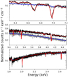 |
Fig. 4. Zoomed spectrum (Top: 6.3–7.2 keV, middle: 3.0–4.5 keV, bottom: 1.8–2.7 keV) for the soft state (data in black and model in red) and hard state (data in grey and model in blue). |
Line parameters for the hard-state observation (obsid:660).
5. Disc wind characterisation
5.1. Phenomenological scaling relations
From Fig. 5 we can see that the profiles of the velocity shift and the velocity width, and the equivalent width of the absorption lines, can be described by a power-law profile (A + B × Eλ) with respect to the ion energies, which are a proxy of the different ionic species and ionisation states. We took positive velocity shift as blueshifted velocity. Within the uncertainties related to the current high-resolution X-ray instruments, it is not possible to decipher a clear non-linear trend, if any. Upcoming high-esolution instruments like XRISM and ATHENA will be able to decipher any non-linear trend (XRISM Science Team 2020; Nandra et al. 2013). The velocity shift is calculated with respect to the line energy calculated by the weighted average of different transitions with respect to their oscillator strength. The velocity width is calculated by Vw = 2.355σc/E0, where c is the speed of light, E0 is the observed energy, Vw is the velocity width, and σ is the line width which is used to estimate the full width at half maximum (FWHM) of the line velocity profile. The parameters of the fit are listed in Table 4. The observed trends can be attributed to different wind ionisation states and different radii at which ions are present.
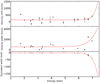 |
Fig. 5. Velocity shift (top), velocity width (middle), and equivalent width (bottom) as a function of line energy for the soft state. In the top panel, the positive velocity shift corresponds to a blueshift. |
Parameters of the power-law fit on velocity shift, velocity width, and equivalent width.
For non-linear profiles of the velocity shift, velocity width, and equivalent width, there can exist multiple components within the outflow. Most lines are consistent with a constant fit and some, particularly Fe XXVI and Fe XXV, show a large deviation. Either different components can be independent or there may be part of the same outflow spread over different radii and ionisation stages. Similar profiles in velocity shift and velocity width have also been seen in GRO J1655-40 by Kallman et al. (2009). In GRO J1655-40 a large part of the outflow has a similar velocity shift to that which we see for GRS 1915+105, with some ions significantly deviating from the constant, similar to the case shown in the present study (Kallman et al. 2009). Fukumura et al. (2017) showed that the non-linear absorption line trend found in GRO J1655-40 was indicative of different segments of the same magnetic outflow. In the following section we explore such a possibility for this source.
5.2. Magnetic disc wind modelling
A magnetic origin of the wind has been suggested by several authors in both AGNs and X-ray binaries (Fukumura et al. 2010, 2017; Blandford & Payne 1982; Contopoulos 1994, 1995; Ferreira 1997). Plasma ejected and accelerated from the disc surface along the poloidal magnetic field lines can give rise to magnetically driven accretion disc winds (Fukumura et al. 2017). This model is mass-invariant in a 2.5D, steady-state and axis-symmetric wind structure for a set of wind parameters. The model accounts for multiple absorption lines simultaneously in a self-consistent manner by modelling the internal structure of the wind, that is, velocity, velocity gradient, density, and ionization. This model can be used to determine the wind structure for a large range of parameters, such as distance, velocity, and density, thus potentially constraining lines from a wide range of ionization states, both in the soft and hard X-ray bands.
The model is comprised of mainly two parts, the poloidal structure of the wind from a geometrically thin accretion disc and the ionisation state of the plasma computed by considering the local heating and cooling balance, and the ionisation equilibrium (Fukumura et al. 2010, 2017). The ionising continuum is assumed to be a point source near the black hole. The model comprises a single continuous wind structure in which different ions at different ionisation states represent different parts of the same outflow. The higher the ionisation, column density, and velocity, the closer the wind component is to the black hole. For a detailed description of the model we refer to Fukumura et al. (2017, 2010). The properties of the wind depend on the inclination angle (θ), ionising spectral energy distribution (SED), and density normalisation (n0) at the innermost launching radius which is assumed to be the innermost stable circular orbit (ISCO) for a Schwarzschild black hole. If the radii (r) and mass flux (ṁ) are scaled by Schwarzschild radius (RS) and Eddington rate (ṀEdd) then the wind density profile can be expressed as n(r) = n0r−p. Consequently, the column density (NH), ionisation potential (ξ), and velocity (v) can be related to each other: NH ∝ ξ(p − 1)/(2 − p), NH ∝ v2(p − 1), v ∝ ξ1/2(2 − p) (Fukumura et al. 2017).
We calculated the detailed wind photo-ionisation structure using the ionising SED derived from extrapolating the observed Chandra unabsorbed continuum in the energy interval between E = 13.6 eV and E = 13.6 keV for both the soft and hard states. However, only the disc blackbody component and the power-law component of the continuum were considered for the SED. We assumed that the wind starts at the ISCO in both the soft and hard states. As the inclination angle is well constrained for this source we fixed the inclination at 70.0 degrees. Major line transitions and edges observable in the X-ray band were implemented using a solar abundance, apart from Fe, S, and Si, where we left the abundances as a free parameter. We varied p and n0 in a self-consistent way. For the fit, n0 was set to vary between 1015 cm−3 and 3.2 × 1018 cm−3, and the density slope p was set to vary between 0.9 and 1.5. For the soft state we got the best fit for p =  (n = n0(r/r0)−1.38), and n0 =
  cm−3 with a χ2 of 4520 for 2631 d.o.f. (Fig. 6). For the hard state, the best fit was obtained for p =
  (n = n0(r/r0)1.378), and n0 =
  cm−3 with a χ2 of 2741 for 2631 d.o.f. Additionally, we also kept the abundances of Fe, S, and Si as variable parameters in the fit. In the soft state we obtained a AS of
  , with a lower limit of 2.92 for AFe and an upper limit of 1.08 for ASi at 90 percent confidence. Similarly, in the hard state we obtained a AFe of
  and lower limits of 2.42 and 2.0 for AS and ASi, respectively, at 90 percent confidence. However, we note that the fit is not very sensitive to the varying abundances and consistent results are also obtained when fixing the values to solar abundances. The broad-band modelling of the soft and hard states using the MHD wind model is shown in Fig. 6. The zoomed-in plot focusing on the Fe XXV and Fe XXVI lines is shown in Fig. 7.
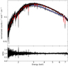 |
Fig. 6. Spectrum of GRS 1915+105 after modelling the absorption lines with the MHD model. Top panel: spectrum of GRS 1915+105 in the soft state and hard state. The data in soft and hard states are plotted in black and grey, while the respective models in red and blue. Bottom panel: Ratio of data and model. |
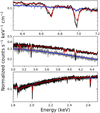 |
Fig. 7. Zoomed (top: 6.3–7.2 keV, middle: 3.0–4.5 keV, bottom: 1.8–2.7 keV) spectrum of GRS 1915+105 in the soft state (data in black and model in red) and hard state (data in grey and model in blue) after modelling with the MHD model. |
6. Discussion and conclusion
In this paper, we investigate the origin of the observed abrupt differences in the wind absorption line properties between the soft and hard states of GRS 1915+105 observed with Chandra HETG. We model the continuum spectra in both states using a black body and power-law emission. We note that this is a phenomenological continuum model and we do not investigate in detail the continuum physical parameters because the main objective of this study is to investigate the narrow absorption features. As a second step, we fit the rich spectrum in the soft state with 20 absorption lines and one emission line using phenomenological Gaussian profiles. A faint Fe XXVI line found in the hard state was also fit with an inverted Gaussian profile.
We find phenomenological scaling relations of the velocity shift, velocity width, and equivalent width of the absorption lines that might follow a non-linear pattern with respect to energy as a tracer of their ionisation, suggesting multiple components in the wind. To explore this scenario further we fitted both the soft- and hard-state spectra using the MHD model that was used for the Chandra HETG spectrum of GRO J1655-40 in Fukumura et al. (2017). We find that, in the soft state, the best fit is obtained with a high-wind-density normalisation (n0 =  cm−3) and for a radial wind density profile (n ∝ r−p) with p ≃ 1.38. Instead, in the hard state, the best-fit values indicate a wind with a low-density normalisation (n0 = (
 cm−3), and a density profile with p ≃ 1.38. The main difference between the two absorption spectra is not dominated by the continuum change but instead it is due to an increase in the wind density by two orders of magnitude going from the hard to the soft state. Our model therefore predicts a persistent presence of disc winds even during hard state, although their spectroscopic appearance is much weaker. This finding suggests that the intrinsic wind condition changes internally with different states of the system, as previously speculated in other sources (Neilsen & Homan 2012; Ponti et al. 2015). This also supports the suggested magnetic origin of the disc wind in GRS 1915+105 (Miller et al. 2015, 2016).
The wind density should in principle be a function of various disc micro physics and magnetic field properties, which are beyond the current state of our model. Fukumura et al. (2014) investigated various types of morphology of MHD winds depending on the plasma property (e.g. the magnetic flux and plasma angular momentum). In this work we assume that the wind morphology remains almost unchanged throughout, considering that the global magnetic field pressure is dominant over radiation pressure in the framework of a generic MHD wind. In this case, the global field lines act like solid rigid wires (e.g. Blandford & Payne 1982) being only weakly sensitive to mass accretion rate. However, it is conceivable that local weak magnetic fields inside the disc, responsible for magneto-rotational instability (MRI), are more intimately coupled to the internal disc structure, and the mass accretion rate and accretion mode may well be a function of those local magnetic fields, while the global magnetic fields are persistent (see Mishra et al. 2020). Therefore, while a large-scale magnetic field structure is essentially unchanged, the cause of the wind density change could be the change in the local magnetic fields within the disc and/or accretion rate. This model is a steady-state calculation that reflects the state of the disc–wind system at a given time. The wind could readjust over its entire range within timescales equal to the viscous time at its outer edge (∼106Rg, where Rg is the Schwarzschild radius) and much faster locally (r ≪ 106Rg), for reasons that are not yet fully understood or taken into account by our calculations. These timescales are of the order of a few days for a black hole of 10 solar masses, which is not inconsistent with the timescale of state transitions in BHBs.
In this model we considered that wind is launched from nearby the ISCO in both the states. Therefore, the characteristics of the MHD wind do not seem to depend strongly on a putative truncation radius of the disc in the hard state. Our fit results suggest that the wind structure changes with respect to the possible state change, and that photo-ionisation alone cannot explain the disappearance of the wind in the hard state, in accordance with the findings of for example Neilsen & Homan (2012) and Ponti et al. (2015). It is conceivable that the change in the wind density may be linked to a change in the accretion disc density, accretion rate, and/or geometry, which is itself responsible for the state change. Chakravorty et al. (2016) claim that a radial power-law profile of accretion rate determines the profile of the outflow, and for a higher power of the profile, the MHD wind is closer to the black hole. Our results are somewhat consistent with the findings of these latter authors, as we assumed a wind starting from ISCO and we obtain a steeper profile in the soft state. Chakravorty et al. (2016) further claim that a wind is not possible in the canonical hard states of BHBs, however the hard state of GRS 1915+105 is peculiar because it does not follow the hysteresis loop in HID as in the case of other LMXBs.
In principle, in the hard state, the wind could also be explained by a thermal origin. However, with the resolution and sensitivity of Chandra HETG, it is not possible to clearly differentiate between these two cases. An upcoming high-resolution micro-calorimeter such as XRISM might be useful to shed more light on these rather controversial issues. Also, in the soft state, we can see that an additional weak component might be required to fit all the lines properly. This could be explained by a second component, possibly a thermal wind. The magnetic and thermal components in the soft state would be consistent with the scenarios put forward by other authors that invoke a multiple-component wind (Miller et al. 2015, 2016). In those scenarios, the magnetic wind might be more variable and the thermal wind could be varying only with respect to the observed continuum. This means that the strong magnetic wind in the soft state was either absent or has become too weak to be detected in the hard state with Chandra HETG, and the thermal wind was present in both the states. This scenario might be similar to the hybrid thermal and magnetic wind suggested by Neilsen & Homan (2012) for GRO J1655-40 in the hard state. In the soft state of GRO J1655-40, the two-component wind found using photo-ionisation modelling by several authors (Kallman et al. 2009; Miller et al. 2006a; Neilsen & Homan 2012) could be a part of a single-component MHD outflow as suggested by Fukumura et al. (2017). However, even in Fukumura et al. (2017), we see that it is possible that a weak additional component might be required for a better fit. Another aspect that we did not incorporate in the spectra is the re-emission from the wind, which is broadened by the Keplerian rotation at the photo-ionisation radius as suggested by Miller et al. (2015, 2016). We will incorporate the re-emission in future work. We find that considering solar abundances we can derive a very good representation of the wind absorption. However, we note that some authors consider the possibility of super solar abundances for some elements when applying more simplistic models (e.g. Ueda et al. 2009). We further estimate the physical parameters of the wind corresponding to the peak distribution of Fe XXVI ions for our best-fit MHD model. As each ion of a given charge state is produced through photo-ionisation over a radially extended distance along the MHD wind, the resultant ionic column is distributed over a finite range of distances. In the following estimates we provide the peak value which refers to the maximum column density and we include the range of values over which a quantity exceeds 50 per cent of the peak value. In the soft state, our best fit returns a FeXXVI peak outflow velocity of  km s−1, an ionisation parameter of log(ξ) =
  erg s−1 cm, and an equivalent hydrogen column density of NH ≃ 1.3 × 1022 cm−2. We estimate the distance of the Fe XXVI absorber from the X-ray source to be log(R/cm) =
  . This does not mean that the launching radius of the wind is at this value, but indicates that the peak of the ionisation parameter corresponds to this radius. Indeed, the MHD model considers a wind launched from a wide range of radii on the disc starting from the ISCO. The absorber located at shorter distances is physically present but is simply unobservable because even iron is fully ionised. In the units of Schwarzschild radius (Rg) the peak radius of Fe XXVI corresponds to R ≃ 1.1 × 10⁷ Rg. At such a large radius the possibility of a thermal wind cannot be ruled out. However, we note that the broad ionisation range seen in the absorption lines, interpreted as a multiple-component outflow by many authors (Miller et al. 2015, 2016), supports a magnetic origin. Indeed, our MHD wind model, in which every single absorber is physically coupled to the same continuous wind, is able to provide a very good representation of the absorption structure of the wind requiring a single stratified MHD disc wind.
A recent study of accretion disc winds in H 1743-32 shows that a thermal wind is preferred to a magnetic wind (Tomaru et al. 2020). However, these latter authors consider only the Fe XXV-XXVI lines and might not be able to characterise a vast amount of soft X-ray lines found in GRS 1915+105. Our MHD model is able to provide a good characterisation of all the absorption lines seen in GRS 1915+105 because it intrinsically considers a stratified wind across the accretion disc. The thermal model in Tomaru et al. (2020), and thermal wind models in general, imply a velocity trend in which the velocity decreases for decreasing launching radius, to the point at which the inner wind is highly ionised and static. Our data on the GRS 1915+105 soft state show the opposite: we have a stratified wind where outflow velocity and the velocity width of the lines increase for increasing ionisation, which is equivalent to saying that the outflow velocity increases for decreasing launching radius. The stratification of the ionisation in the same observation is shown in Miller et al. (2015) as well. Instead, for our hard state observation, in which we only observe a faint Fe XXVI, we cannot exclude the possibility of thermal driving. As suggested above, it is also possible that we have a hybrid situation, with a combination of thermal and MHD wind, with one of the two mechanisms appearing more prominently in different states of the source.
Following Tombesi et al. (2015) and Fukumura et al. (2017), the local mass outflow rate from the wind can be well estimated combining the equation  = 4πmpn(r)r2vout and the definition of the ionisation parameter ξ = LX/n(r)r2, as Ṁout = 4πmpLXvout/ξ. Considering our best-fit Fe XXVI peak parameters and for an ionizing luminosity in the soft state of 4.32 × 1038 ergs s−1 we estimate Ṁout ≃ 2.5 × 10⁻⁹ M⊙ yr−1. The accretion rate, defined as Ṁacc = LX/ηc2, for the source in the soft state is ≃7.7 × 10⁻⁸ M⊙ yr−1 for a typical value of η = 0.1. The estimate of power output through the wind can be derived as ̇E =
  . Integrating the power output throughout the disc, the estimated wind energy output from the system is of the order of one percent of the luminosity.
Upcoming high-energy-resolution instruments like XRISM (XRISM Science Team 2020) and Athena (Nandra et al. 2013) will be able to investigate these matters further. Weaker absorbers, especially in the hard X-ray band (even during hard state if indeed present), can be better probed with the micro-calorimeters in XRISM/Athena. XRISM is planned to be launched in 2022. Here, we test its capabilities to investigate the accretion disc winds in GRS 1915+105 or in sources with similar spectral absorption line features. To this end, we simulated spectra using our best-fit phenomenological models in both soft and hard states. We used the XSPEC “fakeit” command to generate the spectra using an equivalent XRISM calorimeter response with 5 eV energy resolution and the associated background. Figures 8 and 9 show the broadband and Fe K zoomed in XRISM spectra in both the soft and hard states for a short exposure of 10 ks. The accuracy in the line energy, width, and equivalent width for the Fe XXIV-XXVI lines with XRISM will represent more than an order of magnitude improvement compared to Chandra HETG. The line significance for the Fe XXVI, Fe XXV, and Fe XXIV lines in the soft state and Fe XXVI in the hard state will improve on the Chandra HETGS spectra by more than a factor of three. It is to be noted that the exposures for Chandra HETG in the soft and hard states were 49 ks and 30.3 ks compared to the just 10 ks for the simulated XRISM data. Therefore, XRISM will very likely enable a time-resolved study of accretion winds in this and most stellar mass BHBs.
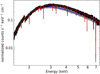 |
Fig. 8. Simulated XRISM spectrum in the same energy band as Chandra HETGS for GRS 1915+105. Here we used the same Chandra HETG best-fit models for the spectra in soft (black) and hard (grey) states. The red and blue lines indicate the fitted phenomenological model. |
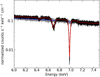 |
Fig. 9. XRISM spectra of GRS 1915+105 zoomed in to the 6.0–7.5 keV energy band. The soft and hard states are indicated in black and grey, respectively. The red and blue lines indicate the fitted phenomenological model. |
It is important to note that X-ray binaries are among the best candidates for detecting X-ray polarisation emission from the disc, the corona, and circumnuclear matter (Dovčiak et al. 2008; Schnittman & Krolik 2009, 2010; Kallman et al. 2015; Taverna et al. 2020). We tested whether or not the absorption lines in the GRS 1915+105 Chandra spectrum can affect the polarisation in the continuum in the context of the upcoming X-ray polarimetry mission IXPE (Weisskopf et al. 2016). We used the IXPEOBSSIM simulator, which takes the spectrum, the polarisation angle, and polarisation degree as a function of energy as input. The polarisation degree and angle as a function of energy for different geometries of the disc and corona have been estimated by some authors (e.g. see Dovčiak et al. 2008). However, for simplicity we considered a constant polarisation angle of 30° and constant polarisation degree of 5%. For the spectrum we used our Chandra soft-state phenomenological model as an input. In one case we used only the continuum, while in a second case we included the absorption lines as well. From this simple test, we can conclude that the presence of unmodelled wind absorption in the soft state of GRS 1915+105 should not hamper the detection of polarisation from the continuum emission. However, the situation may be different if scattering from such a wind is included. As a rough qualitative estimate, considering an MHD wind density profile of n = n0(r/r0)−1.5, the total integrated column density would be NH ≃ 2n0r0, where r0 is of the order of the ISCO. Substituting the ISCO for a non-spinning black hole with the same mass as GRS 1915+105 and a density estimated from our best fits, we find that in the soft state the wind may have a column of up to NH ≃ 4.4×1025 cm−2 in the equatorial direction, while in the hard state it would have a much lower value of NH ≃ 1.1×1024 cm−2. Therefore, the wind may be mostly fully ionised but Compton thick in the equatorial direction in the soft state. Moreover, we note that emission and reflection from the disc wind in X-ray binaries has been suggested (e.g. Miller et al. 2015). This evidence highlights the possibility that some polarised signatures from the wind may be observable with IXPE if the source is caught in the soft state. We defer quantification of the effect of disc winds on the polarised signal in X-rays to a future study.
Acknowledgments
A.R. and F.T. thank J. Neilsen, G. Matt and F. Muleri for the useful comments and discussions. We also thank the anonymous referee for his suggestions in improving this work.
References
- Begelman, M. C., McKee, C. F., & Shields, G. A. 1983, ApJ, 271, 70 [CrossRef] [Google Scholar]
- Belloni, T., Klein-Wolt, M., Méndez, M., van der Klis, M., & van Paradijs, J. 2000, A&A, 355, 271 [Google Scholar]
- Blandford, R. D., & Payne, D. G. 1982, MNRAS, 199, 883 [NASA ADS] [CrossRef] [Google Scholar]
- Castor, J. I., Abbott, D. C., & Klein, R. I. 1975, ApJ, 195, 157 [NASA ADS] [CrossRef] [Google Scholar]
- Chakravorty, S., Petrucci, P. O., Ferreira, J., et al. 2016, Astron. Nachr., 337, 429 [NASA ADS] [CrossRef] [Google Scholar]
- Contopoulos, J. 1994, ApJ, 432, 508 [NASA ADS] [CrossRef] [Google Scholar]
- Contopoulos, J. 1995, ApJ, 450, 616 [NASA ADS] [CrossRef] [Google Scholar]
- Díaz Trigo, M., & Boirin, L. 2016, Astron. Nachr., 337, 368 [NASA ADS] [CrossRef] [Google Scholar]
- Done, C., Tomaru, R., & Takahashi, T. 2018, MNRAS, 473, 838 [NASA ADS] [CrossRef] [Google Scholar]
- Dovčiak, M., Goosmann, R. W., Karas, V., & Matt, G. 2008, in J. Phys. Conf. Ser., 131, 012004 [Google Scholar]
- Fender, R. P., Belloni, T. M., & Gallo, E. 2004, MNRAS, 355, 1105 [NASA ADS] [CrossRef] [Google Scholar]
- Ferreira, J. 1997, A&A, 319, 340 [Google Scholar]
- Fruscione, A., McDowell, J. C., Allen, G. E., et al. 2006, in SPIE Conf. Ser., eds. D. R. Silva, R. E. Doxsey, et al., 6270, 62701V [Google Scholar]
- Fukumura, K., Kazanas, D., Contopoulos, I., & Behar, E. 2010, ApJ, 715, 636 [NASA ADS] [CrossRef] [Google Scholar]
- Fukumura, K., Tombesi, F., Kazanas, D., et al. 2014, ApJ, 780, 120 [Google Scholar]
- Fukumura, K., Kazanas, D., Shrader, C., et al. 2017, Nat. Astron., 1, 0062 [NASA ADS] [CrossRef] [Google Scholar]
- Kallman, T. R., Bautista, M. A., Goriely, S., et al. 2009, ApJ, 701, 865 [NASA ADS] [CrossRef] [Google Scholar]
- Kallman, T., Dorodnitsyn, A., & Blondin, J. 2015, ApJ, 815, 53 [NASA ADS] [CrossRef] [Google Scholar]
- Lee, J. C., Reynolds, C. S., Remillard, R., et al. 2002, ApJ, 567, 1102 [NASA ADS] [CrossRef] [Google Scholar]
- Makishima, K., Maejima, Y., Mitsuda, K., et al. 1986, ApJ, 308, 635 [NASA ADS] [CrossRef] [Google Scholar]
- Martocchia, A., Matt, G., Belloni, T., et al. 2006, A&A, 448, 677 [NASA ADS] [CrossRef] [EDP Sciences] [Google Scholar]
- Miller, J. M. 2006, Astron. Nachr., 327, 997 [NASA ADS] [CrossRef] [Google Scholar]
- Miller, J. M., Raymond, J., Fabian, A. C., et al. 2004, ApJ, 601, 450 [NASA ADS] [CrossRef] [Google Scholar]
- Miller, J. M., Raymond, J., Homan, J., et al. 2006a, ApJ, 646, 394 [NASA ADS] [CrossRef] [Google Scholar]
- Miller, J. M., Raymond, J., Fabian, A., et al. 2006b, Nature, 441, 953 [NASA ADS] [CrossRef] [PubMed] [Google Scholar]
- Miller, J. M., Raymond, J., Reynolds, C. S., et al. 2008, ApJ, 680, 1359 [NASA ADS] [CrossRef] [Google Scholar]
- Miller, J. M., Fabian, A. C., Kaastra, J., et al. 2015, ApJ, 814, 87 [NASA ADS] [CrossRef] [Google Scholar]
- Miller, J. M., Raymond, J., Fabian, A. C., et al. 2016, ApJ, 821, L9 [NASA ADS] [CrossRef] [Google Scholar]
- Miller, J. M., Balakrishnan, M., Reynolds, M. T., et al. 2019, ATel, 12743, 1 [NASA ADS] [Google Scholar]
- Mishra, B., Begelman, M. C., Armitage, P. J., & Simon, J. B. 2020, MNRAS, 492, 1855 [NASA ADS] [CrossRef] [Google Scholar]
- Mitsuda, K., Inoue, H., Koyama, K., et al. 1984, PASJ, 36, 741 [NASA ADS] [Google Scholar]
- Nandra, K., Barret, D., Barcons, X., et al. 2013, ArXiv e-prints [arXiv:1306.2307] [Google Scholar]
- Neilsen, J. 2013, Adv. Space Res., 52, 732 [NASA ADS] [CrossRef] [Google Scholar]
- Neilsen, J., & Lee, J. C. 2009, Nature, 458, 481 [NASA ADS] [CrossRef] [Google Scholar]
- Neilsen, J., & Homan, J. 2012, ApJ, 750, 27 [NASA ADS] [CrossRef] [Google Scholar]
- Neilsen, J., Rahoui, F., Homan, J., & Buxton, M. 2016, ApJ, 822, 20 [NASA ADS] [CrossRef] [Google Scholar]
- Neilsen, J., Cackett, E., Remillard, R. A., et al. 2018, ApJ, 860, L19 [NASA ADS] [CrossRef] [Google Scholar]
- Ponti, G., Fender, R. P., Begelman, M. C., et al. 2012, MNRAS, 422, L11 [NASA ADS] [CrossRef] [Google Scholar]
- Ponti, G., Bianchi, S., Muñoz-Darias, T., et al. 2015, MNRAS, 446, 1536 [NASA ADS] [CrossRef] [Google Scholar]
- Schnittman, J. D., & Krolik, J. H. 2009, ApJ, 701, 1175 [CrossRef] [Google Scholar]
- Schnittman, J. D., & Krolik, J. H. 2010, ApJ, 712, 908 [NASA ADS] [CrossRef] [Google Scholar]
- Taverna, R., Zhang, W., Dovčiak, M., et al. 2020, MNRAS, 493, 4960 [NASA ADS] [CrossRef] [Google Scholar]
- Tomaru, R., Done, C., Ohsuga, K., Odaka, H., & Takahashi, T. 2020, MNRAS, 494, 3413 [NASA ADS] [CrossRef] [Google Scholar]
- Tombesi, F., Cappi, M., Reeves, J. N., et al. 2010, A&A, 521, A57 [NASA ADS] [CrossRef] [EDP Sciences] [Google Scholar]
- Tombesi, F., Meléndez, M., Veilleux, S., et al. 2015, Nature, 519, 436 [NASA ADS] [CrossRef] [Google Scholar]
- Trueba, N., Miller, J. M., Kaastra, J., et al. 2019, ApJ, 886, 104 [NASA ADS] [CrossRef] [Google Scholar]
- Ueda, Y., Murakami, H., Yamaoka, K., Dotani, T., & Ebisawa, K. 2004, ApJ, 609, 325 [NASA ADS] [CrossRef] [Google Scholar]
- Ueda, Y., Yamaoka, K., & Remillard, R. 2009, ApJ, 695, 888 [NASA ADS] [CrossRef] [Google Scholar]
- Weisskopf, M. C., Ramsey, B., O’Dell, S., et al. 2016, in Proc. SPIE, SPIE Conf. Ser., 9905, 990517 [NASA ADS] [CrossRef] [Google Scholar]
- Wilms, J., Allen, A., & McCray, R. 2000, ApJ, 542, 914 [Google Scholar]
- Woods, D. T., Klein, R. I., Castor, J. I., McKee, C. F., & Bell, J. B. 1996, ApJ, 461, 767 [NASA ADS] [CrossRef] [Google Scholar]
- XRISM Science Team 2020, ArXiv e-prints [arXiv:2003.04962] [Google Scholar]
- Zdziarski, A. A., Johnson, W. N., & Magdziarz, P. 1996, MNRAS, 283, 193 [NASA ADS] [CrossRef] [Google Scholar]
- Życki, P. T., Done, C., & Smith, D. A. 1999, MNRAS, 309, 561 [NASA ADS] [CrossRef] [Google Scholar]
Appendix A: Line properties in the soft state
Table A.1 shows the velocity shift, velocity drift, and equivalent width in the soft-state observation (obsid:7485).
Velocity shifts, velocity width, and equivalent width in absorption lines during all observations (obsid:7485).
All Tables
Continuum parameters obtained for the spectral fit for the soft (obsID:7485) and hard (obsID:660) state Chandra observations of GRS 1915+105.
Parameters of the power-law fit on velocity shift, velocity width, and equivalent width.
Velocity shifts, velocity width, and equivalent width in absorption lines during all observations (obsid:7485).
All Figures
|
Fig. 1. Light curve of GRS1915+105 in the soft state (obsid:7485) with a bin size of 100s. |
| In the text | |
|
Fig. 2. Light curve of GRS1915+105 in the hard state with a bin size of 100s (obsid:660). |
| In the text | |
|
Fig. 3. Spectrum of GRS 1915+105 after modelling the absorption and emission lines using the phenomenological Gaussian line profiles. Top panel: spectrum of GRS 1915+105 in the soft state (obsid: 7485) and hard state (obsid: 660). The data in soft and hard states are plotted in black and grey, while the respective models are shown in red and blue. Bottom panel: ratio of data and model. |
| In the text | |
|
Fig. 4. Zoomed spectrum (Top: 6.3–7.2 keV, middle: 3.0–4.5 keV, bottom: 1.8–2.7 keV) for the soft state (data in black and model in red) and hard state (data in grey and model in blue). |
| In the text | |
|
Fig. 5. Velocity shift (top), velocity width (middle), and equivalent width (bottom) as a function of line energy for the soft state. In the top panel, the positive velocity shift corresponds to a blueshift. |
| In the text | |
|
Fig. 6. Spectrum of GRS 1915+105 after modelling the absorption lines with the MHD model. Top panel: spectrum of GRS 1915+105 in the soft state and hard state. The data in soft and hard states are plotted in black and grey, while the respective models in red and blue. Bottom panel: Ratio of data and model. |
| In the text | |
|
Fig. 7. Zoomed (top: 6.3–7.2 keV, middle: 3.0–4.5 keV, bottom: 1.8–2.7 keV) spectrum of GRS 1915+105 in the soft state (data in black and model in red) and hard state (data in grey and model in blue) after modelling with the MHD model. |
| In the text | |
|
Fig. 8. Simulated XRISM spectrum in the same energy band as Chandra HETGS for GRS 1915+105. Here we used the same Chandra HETG best-fit models for the spectra in soft (black) and hard (grey) states. The red and blue lines indicate the fitted phenomenological model. |
| In the text | |
|
Fig. 9. XRISM spectra of GRS 1915+105 zoomed in to the 6.0–7.5 keV energy band. The soft and hard states are indicated in black and grey, respectively. The red and blue lines indicate the fitted phenomenological model. |
| In the text | |
Current usage metrics show cumulative count of Article Views (full-text article views including HTML views, PDF and ePub downloads, according to the available data) and Abstracts Views on Vision4Press platform.
Data correspond to usage on the plateform after 2015. The current usage metrics is available 48-96 hours after online publication and is updated daily on week days.
Initial download of the metrics may take a while.