| Issue |
A&A
Volume 645, January 2021
|
|
|---|---|---|
| Article Number | A128 | |
| Number of page(s) | 15 | |
| Section | Planets and planetary systems | |
| DOI | https://doi.org/10.1051/0004-6361/202039690 | |
| Published online | 29 January 2021 | |
Classification of orbits in three-dimensional exoplanetary systems
1
Department of Physics, School of Science, Aristotle University of Thessaloniki,
541 24
Thessaloniki, Greece
e-mail: evzotos@physics.auth.gr
2
Department of Astronomy, Eötvös University, Pázmány Péter sétány 1/A, 1117
Budapest, Hungary
3
Nonlinear Analysis and Applied Mathematics (NAAM)-Research Group, Department of Mathematics, Faculty of Science, King Abdulaziz University,
PO Box 80203,
Jeddah 21589,
Saudi Arabia
Received:
15
October
2020
Accepted:
11
December
2020
The three-dimensional version of the circular restricted problem of three bodies is utilized to describe a system comprising a host star and an exoplanet. The third body, playing the role of a test particle, can be a comet or an asteroid, or even a small exomoon. Combining the grid classification method with two-dimensional color-coded basin maps, we determine the nature of the motion of the test particle by distinguishing between collision, escaping, and bounded motion. In the case of ordered bounded motion, we also obtain the orientation (retrograde or prograde) as well as the geometry (circulating around one or both of the two main bodies) of the trajectories of the third body, which starts from either the pericenter or apocenter. Following this approach, we are able to systematically explore the dependence of the motion type of the test particle on the initial values of the semimajor axis, eccentricity, and inclination of its orbit.
Key words: methods: numerical / celestial mechanics / planets and satellites: general
© ESO 2021
1 Introduction
In a previous paper (Zotos et al. 2020; hereafter Paper I), we conducted a numerical study on the orbit classification of exoplanetary systems, which was based on the model of the planar, circular restricted three-body problem (CRTBP). In this model, there are two primary bodies (a parent star and an exoplanet or an exoplanet and an exomoon) that move in circular orbits around their common center of mass, and the motion of a third body of negligible mass (an asteroid, comet, or small exomoon) – which is confined to the orbital plane of the primaries – is analyzed. The CRTBP has been widely applied as an approximate model for describing the dynamics of celestial bodies in the Solar System as well as in exoplanetary systems. Its applicability is related to the fact that many orbits are nearly circular in planetary systems. According to The Extrasolar Planets Encyclopaedia1 and the Nasa Exoplanet Archive2, we know of 4284 planets in 3220 planetary systems, of which 712 are multiple planet systems. In contrast with planetary orbits in the Solar System, some orbits in exoplanetary systems are highly eccentric; however, there are 273 planets in single planet systems with zero eccentricity, as well as 59 such planets in 24 of the multiple planet systems.
The dynamics of exoplanets is very complex, and there has been widespread research using various dynamical models, methods, and techniques concerning its different aspects, such as the stability of exoplanetary systems (see e.g., Sándor et al. 2007; Schwarz et al. 2016; Agnew et al. 2017; Carrera et al. 2019; Kane 2019; Marshall et al. 2020), the evolution and role of resonances in multiple planet systems (see e.g., Crida et al. 2008; Antoniadou & Voyatzis 2014; Goździewski et al. 2016; Antoniadou & Libert 2018; Saillenfest et al. 2019), co-orbital dynamics in relation to the search of Trojan exoplanets (see e.g., Érdi & Sándor 2005; Schwarz et al. 2012; Hippke & Angerhausen 2015; Páez & Efthymiopoulos 2015; Leleu et al. 2017), orbital dynamics (see e.g., Hong et al. 2018), and the tidal heating of exomoons (see e.g., Dobos et al. 2017).
In Paper I, we applied the basic dynamical model of the planar CRTBP and the computational methods of Nagler (2004, 2005) to provide a systematic classification (in the form of high-resolution two-dimensional color maps) of the initial conditions that result in bounded, escaping, or collision types of motion; the bounded types were further categorized by their geometry and orientation. We applied the results to several systems of exoplanets whose proper mass parameters were studied in that paper. As initial conditions for the third body, we applied the approach from Érdi et al. (2012), thus considering only launching from the pericenter or apocenter.
Here, we further develop that model and study the three-dimensional CRTBP; as such, the motion of the massless particle is no longer confined to the orbital plane of the primaries. The spatial model is of great theoretical and practical interest, as evidenced by a number of studies. Recently, Schwarz et al. (2012) investigated the linear stability of the libration point L4 in the spatial restricted three-body problem (RTBP), which may have applications to exoplanetary systems. Moreover, Volpi et al. (2019) studied the stability of three-dimensional exoplanetary systems. Antoniadou & Libert (2019) determined resonant three-dimensional periodic solutions in the RTBP. The spatial model proved to be useful in many studies of minor bodies in the Solar System (see e.g., Voyatzis et al. 2018; Morais & Namouni 2019; Gallardo 2020; Kotoulas & Voyatzis 2020). With the advent of the era of detecting minor bodies in exoplanetary systems (see e.g., Zieba et al. 2019), there may be new opportunities to apply the three-dimensional CRTBP.
Our analysis describes the motion of very small bodies (e.g., comets and asteroids) in a star-exoplanet system, which could find further applications in the future. Furthermore, for small values of the initial inclination and at relatively close distances to the exoplanet, the bounded types of motion we study could represent the motion of exomoons around an exoplanet.
This paper is organized as follows: The equations of motion of the applied dynamical model are given in Sect. 2, together with the initial conditions of the studied trajectories. The results of the orbit classification are presented in Sect. 3. The main conclusions of our numerical exploration are summarized in Sect. 4, and the paper ends with Sect. 5, where physical applications of the results are discussed.
2 Dynamical model and initial conditions
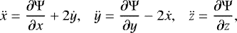
We apply the CRTBP as a dynamical model in our investigations. Here, two massive bodies – labeled B1 (the primary, which is the star) and B2 (the secondary, which is the exoplanet) in Fig. 1 – with masses m1 and m2 orbit in circular trajectories around their common center of mass O, and a third body of negligible mass (a test particle, labeled m) moves under the gravitational influence of the two bodies. The motion of the test particle is not confined to the orbital plane of the star andexoplanet. The three-dimensional motion of the test particle is governed by the following equations of motion (see e.g., Murray & Dermott 1999); they are written in a Cartesian coordinate system, co-rotating with the bodies B1 and B2, where the Oxy plane is the orbital plane of the two bodies and the Ox axis falls on their line, oriented toward the secondary (B2 in Fig. 1):
 (1)
(1)
where Ψ(x, y, z) is the negative effective potential
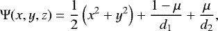 (2)
(2)

Here, x1 = −μ and x2 = 1 − μ are the coordinates of the two main bodies on the x-axis, and m1 = 1 − μ and m2 = μ, where μ ≤ 1∕2 is the mass parameter, defined as μ = m2∕(m1 + m2). Equations (1) are valid in a system of units, where the sum of the mass of the star and the exoplanet, the distance between them, and the constant of gravity is equal to unity. The two main bodies then make one complete revolution in a fixed coordinate system, with the unit angular velocity in 2π time units.
We follow the motion of the test particle by computing its x, y, and z coordinates via numerical integration in the abovementioned barycentric rotating coordinate system. On the other hand, we consider the orbital elements of the test particle orbit with respect to a fixed coordinate system that is centered at the primary (star). We assume that the initial orbital plane of the test particle is inclined to the Oxy plane by an angle i, that the semimajor axis and the direction of the pericenter of its initial elliptic orbit define the x axis of the fixed coordinate system, and that the fixed and rotating x axis coincide at the initial epoch. In this arrangement, we consider two types of initial conditions, corresponding to the pericentric and apocentric launching of the test particle, with the proper pericentric and apocentric velocity (perpendicular to the semimajor axis in the orbital plane) of the initial elliptic motion.
The corresponding initial conditions are
![\begin{align*} &x_0 = {a} \left(1 - e \right) - \mu, \nonumber\\[2pt] &\dot{y_0} = \sqrt{\frac{1 - \mu}{{a}} \frac{1 + e}{1 - e}} \cos\,(i) - {a} \left(1 - e \right), \nonumber\\[2pt] &\dot{z_0} = \sqrt{\frac{1 - \mu}{{a}} \frac{1 + e}{1 - e}} \sin\,(i), &\end{align*}](/articles/aa/full_html/2021/01/aa39690-20/aa39690-20-eq4.png) (4)
(4)
for pericentric launching, and
![\begin{align*} &x_0 = - {a} \left(1 + e \right) - \mu, \nonumber\\[2pt] &\dot{y_0} = - \sqrt{\frac{1 - \mu}{{a}} \frac{1 - e}{1 + e}} \cos\,(i) + {a} \left(1 + e \right), \nonumber\\[2pt] &\dot{z_0} = - \sqrt{\frac{1 - \mu}{{a}} \frac{1 - e}{1 + e}} \sin\,(i), &\end{align*}](/articles/aa/full_html/2021/01/aa39690-20/aa39690-20-eq5.png) (5)
(5)
for apocentric launching; in both cases, 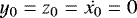 . For i = 0, we obtain the planar initial conditions given in Érdi et al. (2012) and used in Paper I. The initial eccentric trajectory of the massless particle is described through the values of the semimajor axis a, eccentricity e, and inclination i (see Fig. 1).
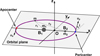 |
Fig. 1 Configuration of the system of the host star B1 and the exoplanet B2. The test particle (labeled m) starts eitherfrom the pericenter or the apocenter of its initial elliptic orbit. |
3 Orbit classification
In what follows, we will determine the influence of the three free parameters of the system (a, e, i), along with that of the mass parameter μ, on the final states of the third body’s trajectories. All the numerical methods (regarding the classification of the starting conditions) and the numerical criteria for distinguishing between the different trajectory types are described in detail in Sect. 3 of Paper I. Wequickly remind the reader that our aim is to distinguish between the escaping, collisional, and bounded motion of the test particle. Moreover, in the case of regular bounded motion, a further classification will be made so as to obtain the geometry (circulation around one or both of the main bodies) and the orientation (retrograde or prograde) of the trajectories. The six main types of regular motion are visually explained in the schematics of Fig. 2.
We mention here that the orientation of the motion refers to the rotating coordinate system. Thus direct (counterclockwise) motion is in the direction of the rotation. Retrograde (clockwise) motion can be retrograde in the rotating system but direct in the fixed system when the launch of the test particle from the pericenter or the apocenter is in the direction of the rotation of the coordinate system. When the launch is in the opposite direction for inclined orbits with inclination above 90°, the motion of the test particle is retrograde in both the rotating and the fixed systems.
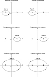 |
Fig. 2 Schematics explaining the main possible configurations of regular orbits around the primaries. |
3.1 The (a, e) survey
The first case under consideration concerns the (a, e)-plane. In Fig. 3 we provide color-coded maps for several values of the initial inclination that correspond to the pericentric launching of the test particle. For the mass parameter, we chose the value μ = 0.001 since it corresponds to a plethora of exoplanetary host star-exoplanet systems (see Table 1 in Paper I).
Here we note that in Fig. 3 (as well as in the subsequent figures), two curves play a decisive role, namely where the pericenter distance dp = a(1 − e) = 1 and where the apocenter distance ap = a(1 + e) = 1. In the fixed coordinate system, both the test particle and the exoplanet orbit around the central star. When dp = 1, the test particle is launched from the vicinity of the exoplanet; due to their close proximity in their following motion, strong perturbations can lead to chaotic motion, or trapped motion around the exoplanet may even occur. When da = 1, during their orbital revolutions around the star, the test particle can approach the exoplanet near its own apocenter, which can lead to strong perturbations and thus dramatic changes in the orbital behavior. To the left of the da = 1 curve, both da and dp are less than 1, and thus the test particle revolves around the star inside the orbit of the exoplanet, at least in the planar case. To the right of the dp = 1 curve, both dp and da are greater than 1, and thus the test particle revolves outside the orbit of the exoplanet and, accordingly, outside the orbits of both the star and the exoplanet. The motion of the test particle is direct in the fixed coordinate system but retrograde in the rotating system since the pericentric velocity of the test particle is smaller than the circular velocity of the exoplanet. (For inclinations above 90°, the motion is retrograde in both systems.) Between the dp = 1 and da = 1 curves, we find that dp < 1 and da > 1; thus the pericenter of the test particle is inside the orbit of the exoplanet and its apocenter is outside (again assuming planar motions, but the description of inclined cases can evolve from this picture). In this region, resonances and various phenomena attached to them (stability, instability, stickiness, escape, chaotic behavior) can play dominant roles since encounters between the test particle and the exoplanet are regulated by the resonances between their motions.
Looking at the maps shown in Fig. 3, it becomes evident that most of the (a, e)-plane is covered by starting conditions corresponding to motion around both primaries. Moreover, for i = 0° and i = 180°, stability islands corresponding to higher order resonant orbits are visible at the tops of the maps. For a > 1, the dominant outer resonances with broad bands are of the n∕1 type, with 2/1 at a = 1.587, 3/1 at a = 2.080, and so on until 10/1 at a = 4.642. Examples ofresonant periodic orbits corresponding to these resonances were shown in Paper I. Families of asymmetric periodic orbits of the 2/1, 3/1, 4/1, and 5/1 outer resonances were computed for Neptune’s mass parameter in Voyatzis et al. (2018). Between the n∕1 resonances, there are others with more narrowwidths, such as 3/2 at a = 1.310, 7/3 at a = 1.759, 7/2 at a = 2.305, 9/2 at a = 2.726, and 11/2 at a = 3.116. Some of these resonances remain for higher inclinations, and even for truly retrograde (i > 90°) orbits. Figure 3 shows that the higher order resonances become dominant with the increase in eccentricity. Families of three-dimensional periodic orbits were computed for the 2/1, 3/2, and 4/3 outer resonances, including both prograde and retrograde orbits, for a mass parameter corresponding to Jupiter’s mass in the CRTBP by Antoniadou & Libert (2018). These resonant periodic orbits were studied for Neptune’s mass parameter in Kotoulas & Voyatzis (2020).
For a = 1, there is the 1/1 resonance. Due to the chosen initial conditions, orbits appearing at a = 1 in Fig. 3 are not librating orbits around the Lagrangian points; rather, they are the planetary types studied in Hadjidemetriou et al. (2009). It is remarkable that such orbits exist for high inclinations as well. Below a = 1, three inner resonances –3/2 at a = 0.763, 2/1 at a = 0.63, and 3/1 at a = 0.481 – are visible in Fig. 3. These were subjects of intensive studies concerning the asteroid belt of the Solar System.
For i = 0° and i = 180°, we see the presence of escaping motion, which is almost entirely absent in all intermediate cases. As the value of the initial inclination of the test particle increases, two main phenomena take place: (i) The amount of trapped chaotic initial conditions, located around the pericenter distance ( ), is reduced; and (ii) the type of regular bounded motion around the host star changes from prograde to retrograde. Ordered motion around the exoplanet is mainly possible for low values of the inclination, while the corresponding starting conditions are mainly situated around the line dp = 1. These correspond to cases where the test particle becomes an exomoon around the exoplanet. Such cases were discussed in Sándor et al. (2007) in the planar elliptic RTBP.
We have similar results in the case of launching from the apocenter, according to the basin diagrams of Fig. 4. The two main differences, with respect to pericentric launching, are the following: (i) The transition between prograde and retrograde motion around the star (Types 1a and 1b) appears at lower initial inclination values; and (ii) the area around the dp = 1 line, containing all the trapped chaotic orbits, is now penetrated, thus allowing the two regions of Type 3a orbits (retrograde trajectories around both primaries) to communicate with each other. It is interesting that for high eccentricities (e > 0.8) resonances of the type 2n∕1 dominate (2/1, 4/1, 6/1, 8/1, 10/1). The resonances that penetrate the dp = 1 line are of the type (2n + 1)∕2, beginning with 3/2 at a = 1.310, 5/2 at a = 1.842, and going up to the very high order 21/2 at a = 4.795. These features are related to the fact that the test particle is launched from the apocenter, from an opposite position to the test particle with respect to the star.
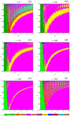 |
Fig. 3 Color-coded basin maps on the (a, e)-plane, when the massless particle starts from its pericenter. The pericenter distances dp and apocenter distances da are marked with dashed white lines and dashed black lines, respectively. |
3.2 The (a, i) survey
The structure of the (a, i)-plane, when μ = 0.001, and for several values of the initial eccentricity e is depicted in Figs. 5 and 6, for pericentric and apocentric launching, respectively. In the case of pericentric launching, it becomes clear that the transition between prograde and retrograde motion around the star occurs near i = 90°. In addition, as the value of the initial eccentricity increases, the number of trapped chaotic orbits grows. At the same time, the unified area of retrograde trajectories around both primaries (Type 3a) starts to split and several stability islands of higher resonant orbits appear for both low and high values of the inclination. It should also be noted that escaping motion is possible only for relatively low values of the inclination (i < 20°). Moreover, initial conditions leading to a collision with the exoplanet are grouped, once more, mainly around the pericentric distance dp = 1. On the other hand, collision with the host star is highly probable for initial conditions near the apocentric distance da = 1 and for values of initial inclination around 90°.
When the test particle starts from its apocenter (see Fig. 6), prograde motion around the host star is less probable and bounded motion around the exoplanet (prograde or retrograde) is almost impossible. It is also noticeable that the presence of resonant motion around both primaries is stronger since the corresponding stability islands are clearer (with respect to what we see in Fig. 5 for the pericentric launching), especially for high values of the initial eccentricity.
3.3 The (e, i) survey
Additional information on the orbital properties of the test particle comes from the basin diagrams on the (e, i)-plane, for fixed values of the mass parameter (μ = 0.001), and the semimajor axis a. In Fig. 7, we present the final states of the massless particle launched from the pericenter with initial conditions on the (e, i)-plane. We observe that for low values of the semimajor axis (see panel a), almost all the available phase space is covered by either prograde or retrograde trajectories around the host star. Additionally, for e > 0.5 and for values of i around 90°, there exists a basin of initial conditions that lead to a collision with the star. On the contrary, when a = 1 (see panel b), the map is roughly divided into two regions that contain: (i) either prograde or retrograde orbits around the exoplanet or (ii) retrograde trajectories around both the star and the exoplanet. For higher values of the semimajor axis (a > 1), the vast majority of the (e, i)-plane is covered by starting conditions of Type 3a orbits, and the second most populated type of motion corresponds to bounded chaotic orbits. Regular motion around the star is no longer possible, and ordered motion around the exoplanet is extremely confined only around the dp = 1 line.
In the case of apocentric launching (see Fig. 8), major differences with respect to the results of Fig. 7 (for the pericentric launching) occur mainly for a = 1. Now bounded regular motion around the exoplanet is no longer possible. For low values of the eccentricity and the inclination, we see a highly complex mixture of chaotic, escaping, and collision orbits, while retrograde motion around the host star is dynamically possible for relatively high values of e (e > 0.8). We also see that the collision with the star basin, around i = 90°, also exists when e > 0.9.
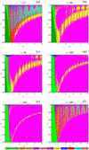 |
Fig. 4 Color-coded basin maps on the (a, e)-plane, when the massless particle starts from its apocenter. The pericenter distances dp and apocenter distances da are marked with dashed white lines and dashed black lines, respectively. |
3.4 The (μ, e) survey
All the results so far correspond to a mass parameter μ = 0.001. However, it would be interesting to see how this parameter also affects the nature of the three-dimensional motion of the test particle.
The maps on the (μ, e)-plane for several values of the inclination and for pericentric launching are given in Fig. 9, where a = 0.5. It is seen that for zero inclination the structure of the phase space is highly complicated, containing complicated escape and collision basins along with regions of bounded motion. In this case, the bounded motion is either chaotic or prograde around the host star. With increasing values of the inclination, the orbital structure of the (μ, e)-plane becomes simpler since all the complicated basins of collision seem to weaken significantly. At the same time, the number of resulted bounded orbits increases, and their orientation changes from prograde to retrograde. At the highest studied value of inclination (see panel f), basins of retrograde motion around the star cover almost half of the (μ, e)-plane, and the rest is occupied by escaping orbits and starting conditions that mainly lead to a collision with the host star.
The diagrams in Fig. 10 also corresponds to pericentric launching, but this time the value of the semimajor axis is a = 5. Once more, the most complicated structures correspond to the scenario with i = 0° (see panel a). We see that for high values of a, bounded motion around the host star is no longer possible. On the other hand, the vast majority of regular trajectories correspond to retrograde motion around both primaries, and bounded motion (both prograde and retrograde) around the exoplanet is possible with starting conditions along the pericenter line dp = 1. It is also interesting to note that regular motion around both the exoplanet and the host star exists mainly for dp < 1.
The case of apocentric launching with a = 0.5 is presented in the color-coded maps of Fig. 11. Again, for a zero value of the inclination (see panel a), we have the most complicated orbital content. Regarding the initial value of the inclination, we observe in all six cases that the most probable types of motion are bounded motion (either prograde or retrograde) around the host star, escaping, or collision motion toward the star. On thecontrary, there is no indication of ordered bounded motion around the exoplanet, and collision with it seems very unlikely.
The last case under consideration deals with apocentric launching with a = 5. According to the basins diagrams of Fig. 12, the test particle in this case can either be on regular trajectories around boththe star and the exoplanet or it escapes from the system. Collision with the star or the exoplanet is also possible, though less probable. In particular, collision motion seems to be more likely when the initial inclination of the test particle is either 0 or 180 degrees. We also see that for low values of the inclination there is a unified stability island corresponding to Type 3a trajectories (retrograde around both primaries). However, as the value of the inclination increases, this stability island initially grows in size and eventually breaks into two sub-islands. When i = 180°, all the complicated basins of collision evolve between these two stability islands.
We have seen that the most complicated basin structures appear at the (μ, e)-plane for i = 0°. To provide a more quantitative estimate on this, we computed the uncertainty (fractal) dimension (see e.g., Aguirre et al. 2001, 2009) of the corresponding basin diagrams. It was found that the uncertainty dimension D0 in these cases is on the order of 1.75–1.82, while in all other studied cases (in other types of basin diagrams) it is always less than 1.6. We note that when the value of D0 is close to 1 in a two-dimensional basin diagram, it implies zero fractality, while when D0 tends to 2 we have the case of total fractality.
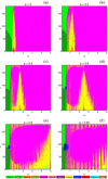 |
Fig. 5 Color-coded basin maps on the (a, i)-plane, when the massless particle starts from its pericenter. The pericenter distances dp and apocenter distances da are marked with dashed white lines and dashed black lines, respectively. |
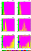 |
Fig. 6 Color-coded basin maps on the (a, i)-plane, when the massless particle starts from its apocenter. The pericenter distances dp and apocenter distances da are marked with dashed white lines and dashed black lines, respectively. |
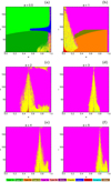 |
Fig. 7 Color-coded basin maps on the (e, i)-plane, when the massless particle starts from its pericenter. The pericenter distances dp and apocenter distances da are marked with dashed white lines and dashed black lines, respectively. |
4 Concluding remarks
In this paper, we expanded the work initiated in Paper I into three dimensions. By utilizing the spatial version of the restricted circular problem of three bodies (describing a system of a host star and an exoplanet), we determined the final states of a test particle that could be an asteroid, a comet, or even a small exomoon. Combining the grid classification method with two-dimensional color-coded basin maps, we were able to study the nature of motion of the test particle by distinguishing between collision, escaping, and bounded motion. Moreover, in the case of ordered bounded motion, we also obtained the orientation (retrograde or prograde) as well as the geometry (circulating around one or both of the two main bodies) of the trajectories of the third body. We also considered two cases regarding the launching of the test particle: starting from its pericenter or apocenter.
The color-coded two-dimensional basin maps revealed the following results regarding the influence of the free parameters of the system (a, e, i, μ):
-
Regular bounded motion around the host star (either prograde or retrograde) exists mainly when the initial value of the semimajor axis of the test particle is lower than 1. Prograde motion around the star is more probable for i < 90°, while retrograde motion around the same primary appears for i > 90°.
-
Regular bounded motion around the exoplanet (either prograde or retrograde) corresponds to initial conditions that are organized around the pericenter line dp = 1.
-
Retrograde ordered motion around both primaries (host star and exoplanet) occurs mainly for a > 1, while prograde motion of the same type is not possible, at least for the particular launching of the test particle.
-
Collision motion is highly probable for i = 0° and i = 180°. For all intermediate values of the inclination, collision with primaries is still possible; however, the corresponding starting conditions do not form basins of collision.
-
In general terms, regular bounded motion occurs mainly for e < 0.5, while forhigher initial values of the eccentricity, ordered motion is less probable and escaping and/or collision motion dominates.
The motion equations were integrated numerically using a Bulirsch-Stoer algorithm with double precision developed in FORTRAN 77 (e.g., Press et al. 1992). The energy integral was sufficiently conserved during the procedure of the numerical integration, with a relative error on the order of 10−12 (or even smaller in some cases). A Quad-Core Intel i7 5.0 GHz processor was used for the orbit classification, and the required CPU time (per grid of starting conditions) varied between 0.5 and 27 hr, depending strongly on the amount of escaping and collision trajectories. All the color-coded maps were designed using MathematicaⓇ software (Wolfram 2003).
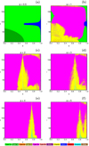 |
Fig. 8 Color-coded basin maps on the (e, i)-plane, when the massless particle starts from its apocenter. The pericenter distances dp and apocenter distances da are marked with dashed white lines and dashed black lines, respectively. |
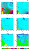 |
Fig. 9 Color-coded basin maps on the (μ, e)-plane, when the massless particle starts from its pericenter, with a = 0.5. The pericenter distances dp and apocenter distances da are marked with dashed white lines and dashed black lines, respectively. |
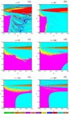 |
Fig. 10 Color-coded basin maps on the (μ, e)-plane, when the massless particle starts from its pericenter, with a = 5. The pericenter distances dp and apocenter distances da are marked with dashed white lines and dashed black lines, respectively. |
5 Physical applications
In recent years, the search for exomoons has been a very active field. The most important project is the so-called Hunt for Exomoonswith Kepler (HEK), which uses several techniques for exomoon detection (Kipping et al. 2013, 2014, 2015). So far, the best exomoon candidate obtained from HEK is Kepler 1625b, which has a Jupiter-like host exoplanet and a Sun-like parent star (Teachey & Kipping 2018). However, it was very recently announced that six more exomoons may have been spotted (Fox & Wiegert 2021). The six exoplanet candidates that might contain exomoons are: KOI 268.01, Kepler 517b, Kepler 1000b, Kepler 409b, Kepler 1326b, and Kepler 1442b.
Theoretically, all exomoons must have relatively low values of inclination i ∈ [0°, 15°]. However, Teachey & Kipping (2018) postulate that a possible exomoon orbiting Kepler-1625b may have an inclination of 45°. On this basis, we can argue that our results, presented in Sect. 3, can have direct applications to exomoon dynamics. In particular, all the basins of regular motion that appear in the color-coded maps of Sect. 3 may correspond to stable regular motion of exomoons around exoplanets (corresponding to Types 2a and 2b), or even of very small additional exoplanets around the parent star (corresponding to Types 1a and 1b). Moreover, the same diagrams can predict fugitive exomoons or exoplanets following escaping orbits, or even doomed celestial bodies that result in a collision with either the exoplanet or the parent star.
Our numerical analysis also contains cases where the initial inclination of the test particle has higher values, covering the full range between 0° and 180°. These cases may describe the motion of extremely small particles, such as comets, asteroids, or even space probes, moving inside the combined gravitational field of the parent star and the exoplanet.
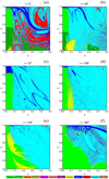 |
Fig. 11 Color-coded basin maps on the (μ, e)-plane, when the massless particle starts from its apocenter, with a = 0.5. The pericenter distances dp and apocenter distances da are marked with dashed white lines and dashed black lines, respectively. |
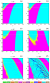 |
Fig. 12 Color-coded basin maps on the (μ, e)-plane, when the massless particle starts from its apocenter, with a = 5. The pericenter distances dp and apocenter distances da are marked with dashed white lines and dashed black lines, respectively. |
Acknowledgments
The authors thankfully acknowledge the Deanship of Scientific Research (DSR) at King Abdulaziz University, for funding this project, under grant number KEP-17-130-41. The authors would also like to express their warmest thanks to the anonymous referee for the careful reading of the manuscript as well as for all the apt suggestions and comments which allowed us to improve both the quality and the clarity of the paper.
References
- Agnew, M. T., Maddison, S. T., Thilliez, E., & Horner, J. 2017, MNRAS, 471, 4494 [NASA ADS] [CrossRef] [Google Scholar]
- Aguirre, J., Vallejo, J. C., & Sanjuán, M. A. F. 2001, Phys. Rev. E, 64, 066208 [NASA ADS] [CrossRef] [Google Scholar]
- Aguirre, J., Viana, R. L., & Sanjuán, M. A. F. 2009, Rev. Mod. Phys., 81, 333 [NASA ADS] [CrossRef] [Google Scholar]
- Antoniadou, K. I., & Libert, A. S. 2018, A&A, 615, 60 [NASA ADS] [CrossRef] [EDP Sciences] [Google Scholar]
- Antoniadou, K. I., & Libert, A. S. 2019, MNRAS, 483, 2923 [NASA ADS] [CrossRef] [Google Scholar]
- Antoniadou, K. I., & Voyatzis, G. 2014, Ap&SS 349, 657 [NASA ADS] [CrossRef] [EDP Sciences] [Google Scholar]
- Carrera, D., Raymond, S. N., & Davies, M. B. 2019, A&A, 629, L7 [NASA ADS] [CrossRef] [EDP Sciences] [Google Scholar]
- Crida, A., Sándor, Z., & Kley, W. 2008, A&A, 483, 325 [NASA ADS] [CrossRef] [EDP Sciences] [Google Scholar]
- Dobos, V., Heller, R., & Turner, E. I. 2017, A&A, 601, 91 [Google Scholar]
- Érdi, B., & Sándor, Zs. 2005 Celest. Mech. Dyn. Astron., 92, 113 [NASA ADS] [CrossRef] [Google Scholar]
- Érdi, B., Rajnai, R., Sándor, Z., & Forgács-Dajka, E. 2012, Celest. Mech. Dyn. Astron., 113, 95 [NASA ADS] [CrossRef] [Google Scholar]
- Fox, C., & Wiegert, P. 2021, MNRAS, 501, 2378 [NASA ADS] [CrossRef] [Google Scholar]
- Gallardo, T. 2020, Celest. Mech. Dyn. Astron., 132, 9 [Google Scholar]
- Goździewski, K., Migaszewski, C., Panicki, F., & Szuszkiewicz, E. 2016, MNRAS, 455, 104 [NASA ADS] [CrossRef] [Google Scholar]
- Hadjidemetriou, J. D., Psychoyos, D., & Voyatzis, G. 2009, Celest. Mech. Dyn. Astron., 104, 23 [NASA ADS] [CrossRef] [Google Scholar]
- Hippke, M., & Angerhausen, D. 2015, ApJ, 811, 5 [NASA ADS] [CrossRef] [Google Scholar]
- Hong, Y. C., Raymond, S. N., Nicholson, P. D., & Lunine, J. I. 2018, ApJ, 852, 85 [NASA ADS] [CrossRef] [Google Scholar]
- Kane, S. R. 2019, AJ, 158, 72 [NASA ADS] [CrossRef] [Google Scholar]
- Kipping, D. M., Forgan, D., & Hartman, J., et al. 2013, ApJ, 777, 134 [NASA ADS] [CrossRef] [Google Scholar]
- Kipping, D. M., Nesvorný, D., & Buchhave, L. A., et al. 2014, ApJ, 784, 28 [NASA ADS] [CrossRef] [Google Scholar]
- Kipping, D. M., Schmitt, A. R., & Huang, X., et al. 2015, ApJ, 813, 14 [NASA ADS] [CrossRef] [Google Scholar]
- Kotoulas, T., & Voyatzis, G. 2020, Celest. Mech. Dyn. Astron., 132, 33 [NASA ADS] [CrossRef] [Google Scholar]
- Leleu, A., Robutel, P., Correia, A. C. M., & Lillo-Box, J. 2017, A&A, 599, 4 [CrossRef] [EDP Sciences] [Google Scholar]
- Marshall, J. P., Horner, J., Wittenmyer, R. A., Clark, J. T., & Mengel, M. W. 2020, MNRAS, 494, 2280 [NASA ADS] [CrossRef] [Google Scholar]
- Morais, M. H. M., & Namouni, F. 2019, MNRAS, 490, 3799 [CrossRef] [Google Scholar]
- Murray, C., & Dermott, S. 1999, Solar System Dynamics (Cambridge: Cambridge Univesristy Press) [Google Scholar]
- Nagler, J. 2004, Phys. Rev. E, 69, 066218 [NASA ADS] [CrossRef] [EDP Sciences] [Google Scholar]
- Nagler, J. 2005, Phys. Rev. E, 71, 026227 [NASA ADS] [CrossRef] [Google Scholar]
- Páez, R. I., & Efthymiopoulos, C. 2015, Celest. Mech. Dyn. Astron., 121, 139 [NASA ADS] [CrossRef] [Google Scholar]
- Press, H. P., Teukolsky, S. A, Vetterling, W. T., & Flannery, B. P. 1992, Numerical Recipes in FORTRAN, 2nd edn. (Cambridge, USA: Cambridge University Press) [Google Scholar]
- Saillenfest, M., Laskar, J., & Boué, G. 2019, A&A, 623, 4 [Google Scholar]
- Sándor, Z., Süli, Á., Érdi, B., Pilat-Lohinger, E., & Dvorak, R. 2007, MNRAS, 375, 1495 [NASA ADS] [CrossRef] [Google Scholar]
- Schwarz, R., Bazsó, Á., Érdi, B., & Funk, B. 2012, MNRAS, 427, 397 [NASA ADS] [CrossRef] [Google Scholar]
- Schwarz, R., Funk, B., Zechner, R., & Bazsó, Á. 2016, MNRAS, 460, 3598 [NASA ADS] [CrossRef] [Google Scholar]
- Teachey, A., & Kipping, D. M. 2018, Sci. Adv., 4, 10 [NASA ADS] [CrossRef] [Google Scholar]
- Volpi, M., Arnaud, R., & Libert, A. S. 2019, A&A, 626, A74 [CrossRef] [EDP Sciences] [Google Scholar]
- Voyatzis, G., Tsiganis, K., & Antoniadou, K. I. 2018, Celest. Mech. Dyn. Astron., 130, 29 [NASA ADS] [CrossRef] [Google Scholar]
- Wolfram, S. 2003, The Mathematica Book (Champaign: Wolfram Media) [Google Scholar]
- Zieba, S., Zwintz, K., Kenworthy, M. E., & Kennedy, G. M. 2019, A&A, 625, A13 [Google Scholar]
- Zotos, E. E., Érdi, B., Saeed, T., & Alhodaly, M. Sh. 2020, A&A, 634, 60 (Paper I) [CrossRef] [EDP Sciences] [Google Scholar]
All Figures
|
Fig. 1 Configuration of the system of the host star B1 and the exoplanet B2. The test particle (labeled m) starts eitherfrom the pericenter or the apocenter of its initial elliptic orbit. |
| In the text | |
|
Fig. 2 Schematics explaining the main possible configurations of regular orbits around the primaries. |
| In the text | |
|
Fig. 3 Color-coded basin maps on the (a, e)-plane, when the massless particle starts from its pericenter. The pericenter distances dp and apocenter distances da are marked with dashed white lines and dashed black lines, respectively. |
| In the text | |
|
Fig. 4 Color-coded basin maps on the (a, e)-plane, when the massless particle starts from its apocenter. The pericenter distances dp and apocenter distances da are marked with dashed white lines and dashed black lines, respectively. |
| In the text | |
|
Fig. 5 Color-coded basin maps on the (a, i)-plane, when the massless particle starts from its pericenter. The pericenter distances dp and apocenter distances da are marked with dashed white lines and dashed black lines, respectively. |
| In the text | |
|
Fig. 6 Color-coded basin maps on the (a, i)-plane, when the massless particle starts from its apocenter. The pericenter distances dp and apocenter distances da are marked with dashed white lines and dashed black lines, respectively. |
| In the text | |
|
Fig. 7 Color-coded basin maps on the (e, i)-plane, when the massless particle starts from its pericenter. The pericenter distances dp and apocenter distances da are marked with dashed white lines and dashed black lines, respectively. |
| In the text | |
|
Fig. 8 Color-coded basin maps on the (e, i)-plane, when the massless particle starts from its apocenter. The pericenter distances dp and apocenter distances da are marked with dashed white lines and dashed black lines, respectively. |
| In the text | |
|
Fig. 9 Color-coded basin maps on the (μ, e)-plane, when the massless particle starts from its pericenter, with a = 0.5. The pericenter distances dp and apocenter distances da are marked with dashed white lines and dashed black lines, respectively. |
| In the text | |
|
Fig. 10 Color-coded basin maps on the (μ, e)-plane, when the massless particle starts from its pericenter, with a = 5. The pericenter distances dp and apocenter distances da are marked with dashed white lines and dashed black lines, respectively. |
| In the text | |
|
Fig. 11 Color-coded basin maps on the (μ, e)-plane, when the massless particle starts from its apocenter, with a = 0.5. The pericenter distances dp and apocenter distances da are marked with dashed white lines and dashed black lines, respectively. |
| In the text | |
|
Fig. 12 Color-coded basin maps on the (μ, e)-plane, when the massless particle starts from its apocenter, with a = 5. The pericenter distances dp and apocenter distances da are marked with dashed white lines and dashed black lines, respectively. |
| In the text | |
Current usage metrics show cumulative count of Article Views (full-text article views including HTML views, PDF and ePub downloads, according to the available data) and Abstracts Views on Vision4Press platform.
Data correspond to usage on the plateform after 2015. The current usage metrics is available 48-96 hours after online publication and is updated daily on week days.
Initial download of the metrics may take a while.