| Issue |
A&A
Volume 645, January 2021
|
|
|---|---|---|
| Article Number | A63 | |
| Number of page(s) | 16 | |
| Section | Celestial mechanics and astrometry | |
| DOI | https://doi.org/10.1051/0004-6361/202039617 | |
| Published online | 15 January 2021 | |
Dynamics of charged dust in the orbit of Venus
1
School of Astronomy and Space Science, Nanjing University,
163 Xianlin Avenue,
Nanjing 210046,
PR China
e-mail: This email address is being protected from spambots. You need JavaScript enabled to view it.
2
Institute of Astrophysics, University of Vienna,
Türkenschanzstrasse 17,
1180 Vienna, Austria
e-mail: This email address is being protected from spambots. You need JavaScript enabled to view it.
3
Key Laboratory of Modern Astronomy and Astrophysics in Ministry of Education, Nanjing University,
Nanjing 210046,
PR China
4
Space Research Institute, Austrian Academy of Sciences,
Schmiedlstrasse 6,
8042 Graz, Austria
5
Department of Mathematics, University of Rome Tor Vergata,
Via della Ricerca Scientifica 1,
00133 Roma, Italy
6
Faculty of Mathematics, ‘Al. I. Cuza’ University of Iasi,
Bd. Carol I., 11,
7000506 Iasi, Romania
7
Institute of Space Astronomy and Extraterrestial Exploration (NJU & CAST), Nanjing 210046,
PR China
Received:
8
October
2020
Accepted:
4
December
2020
Abstract
We study the dynamics of co-orbital dust in the inner Solar System, that is, the role of the solar radiation pressure, the Poynting-Robertson effect, the solar wind, and the interplanetary magnetic field, on the location, width, and stability of resonant motion of charged and micron-sized dust grains situated in the 1:1 mean motion resonance with Venus. We find deviations and asymmetry between L4 and L5 in the locations of the libration centers and libration width caused by nongravitational effects with analytical and numerical methods. The triangular Lagrangian points become unstable when solar radiation pressure, the Poynting-Robertson effect, and solar wind drag are considered. The Lorentz force could further destabilize the orbits, especially for small dust particles. We also compare the circular and/or elliptic restricted three-body model and a more complete model that includes all planets.
Key words: zodiacal dust / methods: analytical / methods: numerical / planets and satellites: individual: Venus / Sun: heliosphere / chaos
© ESO 2021
1 Introduction
Measurements of the Venera 9 and 10 spacecraft (Krasnopolsky & Krysko 1979) served as first evidence for a co-orbital dust ring around Venus. These measurements were tested later by the Helios mission (Leinert & Moster 2007) and were confirmed with observations from STEREO (Jones et al. 2013, 2017). In Pokorný & Kuchner (2019) the total amount of material within the dust ring was estimated to be about 1.3 × 10¹³ kg, which corresponds to an equivalent of an asteroid of about 2 km in diameter (assuming a mean bulk density of 3 g cm−3). According to the authors, the analysis of the measurements of the STEREO spacecraft shows that the ring is spread within a region of a radial width equal 0.06 AU and a height of 0.1 AU. The question now is where it comes from. If the dust ring of Venus is not a temporary phenomenon (e.g., caused by comets passing the inner Solar System), it must be continuously filled up with new material either from the interplanetary medium or from the erosion of some primordial Venus Trojans (Pokorný & Kuchner 2019).
The capture probability of dust in co-orbital resonance with Venus is rather low (Jeong & Ishiguro 2012), but still possible (Jackson & Zook 1989), and it is also known to exist for the other planets, for example, Earth (Dermott et al. 1994) or Jupiter (Lhotka & Celletti 2015). It has been shown that the capture process into mean motion resonance (MMR) between a dust particle and a planet strongly depends on the order of the resonance. It is well known that capture within the orbit of the perturber is not possible but can take place for outer resonances (Sicardy et al. 1993; Beauge & Ferraz-Mello 1994; Liou & Zook 1995). Low capture probabilities are not the only problem that needs to be solved to explain the dust ring of Venus. Capture is also known to be a phenomenon, but it is only temporal (Lhotka & Celletti 2015; Lhotka & Gales, 2019). The reason is found in the effect of nongravitational perturbations, that is, solar wind drag and the force of the so-called Poynting-Robertson effect (Klačka et al. 2014): micron-sized dust particles in the Solar System experience a net drift toward the inner part of the Solar System through loss of orbital energy that leads to a shrinking of the semimajor axes. The drift is canceled in (outer or co-orbital) resonance for finite times, but because of nonlinear perturbations, the particle starts librating with increasing amplitude around the exact resonance condition, until it is removed and again starts drifting (in radial distance) toward the Sun.
We here mainly investigate the timescales of temporary capture of micron-sized dust grains that are in co-orbital resonance with Venus. We also provide a detailed analysis of the location of the exact resonance that depends, as we show, on various parameters: the size and the charge of the dust grains, the interplanetary magnetic field strength and so on. We focus in particular on some nongravitational effect that is usually neglected in this type of studies: the role of charge in the interplanetary magnetic field. The resulting Lorenz force may strongly affect the dynamics, as has previously been shown for micron-sized particles out of resonance (Lhotka et al. 2016) and in outer MMRs with Jupiter (Lhotka & Gales, 2019). While in the former study the authors find suitable conditions under which the drift in semimajor axes of micron-sized dust grains is reduced as a result of the normal component of the interplanetary magnetic field, a reduction in capture time has been found in Lhotka & Gales (2019) from the enhancement of chaotic regions close to resonance because of acharge. We therefore investigate the shift in equilibria and time of temporary capture in the case of co-orbital motions of charged dust grains with Venus, including the important effect of the interplanetary magnetic field.
We state the models and methods that we used in Sect. 2. The dynamical behavior of uncharged particles in 1:1 MMR is studied both analytically and numerically in Sect. 3. The effect of the Lorentz force resulting from the interplanetary magnetic field is described in detail in Sect. 4. We present a summary and the discussion of our study in Sect. 5. Further mathematical details related to the analytical study, including a more general formula for the shift in location of the co-orbital resonance caused by nongravitational effects and the second-order solution to the characteristic equation in linear stability analysis, can be found in the appendices.
2 Model and method
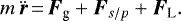
In the absence of nongravitational forces, the only perturbations of the dust grain orbits are due to additional planets and the problem reduces to the standard N-body problem. In the case of only one perturber, that is, Venus, the problem further reduces to the restricted three-body problem, which serves as a prototype model in Solar System dynamics. Depending on the geometry of the perturber’s (Venus) orbit the planar or inclined, circular or elliptic three-body problems may be defined. These models serve as the basis for our investigations (Dvorak & Lhotka 2013). However, when we consider dust grain dynamics in the Solar System, nongravitational effects can usually not be neglected (Burns et al. 1979). The dust grain orbits are strongly affected by the conjugated effects of the solar radiation and solar wind. Let r be the position of a dust grain in the heliocentric coordinate system. Assuming the dust grain to be a spherical object of radius R, let m be its mass, A = πR2 the cross-sectional area exposed to sunlight, ρ the mass density, and q the charge. The parameters are related by m = 4πρR3∕3 and q = 4πε0UR with surface potential U and electric constant ε0. As we show below, the strength of the nongravitational effects is proportional to 1∕R (obtained from the area-to-mass ratio), and U∕R2 (obtained from the charge-to-mass ratio), respectively. In this section we essentially follow the mathematical treatment in Lhotka & Gales (2019), where the equation of motion for a test particle is provided by Eq. (1) therein:
 (1)
(1)
Here Fg indicates the gravity of the Sun and additional bodies; Fs∕p is the force induced by the interaction of the dust grain with solar radiation and solar wind, and FL is the Lorentz force. For a complete treatment of the model, see Lhotka & Gales (2019). We only report the formalism related to the nongravitational effects that we used.
2.1 Solarradiation pressure, the Poynting-Robertson effect, and solar wind drag
According to Klačka et al. (2012, 2014), the force caused by solar radiation pressure, the Poynting-Robertson effect, and solar wind drag can be expanded up to first order in v∕c as
![Mathematical equation: \begin{equation*}{\vec{F}_{s/p}}\,{=}\,-\nabla\frac{\mu\,m\,\beta}{r}-\frac{\mu\,m\,\beta}{r^2}\left(1+s_w\right)\left[\frac{(\vec{\dot{r}} \cdot\vec{r})\,\vec{r}}{c\,r^2}+\frac{\vec{\dot{r}}}{c}\right], \end{equation*}](/articles/aa/full_html/2021/01/aa39617-20/aa39617-20-eq2.png) (2)
(2)
where v is the velocity of the particle and c is the speed of light, ∇ is the gradient operator, μ is the mass of the Sun, β is the ratio between the magnitudes of the solar radiation pressure and gravity, ṙ is the velocity vector of the particle relative to the Sun, r indicates the distance to the Sun, and sw is the ratio of solar wind drag to Poynting-Robertson effect.
The first term in Eq. (2), which corresponds to the solar radiation pressure, can be expressed as the gradient of a potential proportion to gravitational potential. Therefore we incorporate this term into the Kepler motion by assigning the Sun a reduced mass of (1 − β) μ when we consider the solar radiation pressure for particles. Because the force induced by the solar wind is similar to that from Poynting-Robertson effect but has a different coefficient sw, we denote the combined effect of them as P-R-S effect hereafter.
2.2 Lorentz force
The interplanetary magnetic field has an Archimedian spiral field line pattern because the solar wind plasma takes the magnetic field radially away from the Sun, and in addition, the solar rotation winds the field lines around the rotation axis. The spiral field pattern is also referred to as the Parker spiral. The magnetic field can be oriented away from the Sun (the “away” sector) or toward the Sun (the “toward” sector), depending on how the coronal field lines are configurated. In interplanetary space near the ecliptic plane, the interplanetary magnetic field typically has a four-sector structure, which comes from an ecliptic section of the curved shaped of the magnetic equator of the Sun. In response to the solar magnetic field, the interplanetary magnetic field roughly exhibits a 22-yr cycle such that the magnetic polarity reverses in every solar cycle with 11 yr.
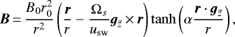
The Parker spiral model (Webb et al. 2010; Bieber et al. 1987) is adopted in this paper to describe the interplanetary magnetic field. We follow the simplified analytic expression in Lhotka & Gales (2019),
 (3)
(3)
where B0 is the background magnetic field strength given at the reference distance r0, Ωs indicates the solar rotation rate, and usw is the radial speed of the solar wind, α is a positive parameter determining the shape of the sign change function f(ϕ) = tanh(αϕ), and  is the unit vector pointing to the rotation axis of the Sun and can be defined by
![Mathematical equation: \begin{equation*} {\vec{g}_{\tilde{z}}}\,{=}\,\sin(i_0)\left[\sin(\Omega_0){\vec{g}_x}-\cos(\Omega_0){\vec{g}_y}\right]+\cos(i_0){\vec{g}_z}, \end{equation*}](/articles/aa/full_html/2021/01/aa39617-20/aa39617-20-eq5.png) (4)
(4)
where i0 is the angle between solar equator and the ecliptic plane, and Ω0 is the ecliptic angle difference between the direction of the vernal equinox and the line of nodes between the equatorial and ecliptic planes. Following Lhotka & Gales (2019), {gx, gy, gz} represents the basis of heliocentric reference frame, where gz points to the ecliptic pole, gx is aligned with the direction to the vernal equinox, and gy is determined by the right-handed rule.
Hence in the heliocentric ecliptic reference frame, the Lorentz force FL is (Lhotka & Gales, 2019)
![Mathematical equation: \begin{eqnarray*}{\vec{F}_{\textrm{L}}}&\,{=}\,&{-}\frac{qB_0r_0^2}{r^2}\left[\frac{1}{r}\vec{r}\,{\times}\,\vec{\dot{r}}+\frac{\Omega_s}{r}\vec{r}\,{\times}\,(\vec{r}\,{\times}\,{\vec{g}_{\tilde{z}}})+\frac{\Omega_s}{u_{\textrm{sw}}}(\vec{r}\,{\times}\,{\vec{g}_{\tilde{z}}})\,{\times}\,\vec{\dot{r}}\right]\nonumber\\ &&{\times}\,\tanh\left(\alpha\frac{\vec{r}\cdot{\vec{g}_{\tilde{z}}}}{r}\right). \end{eqnarray*}](/articles/aa/full_html/2021/01/aa39617-20/aa39617-20-eq6.png) (5)
(5)
In addition to the position and velocity, the acceleration caused by the Lorentz force is mainly dependent on the charge-to-mass ratio q∕m of particles.
We note that the interplanetary magnetic field given by Eq. (3) does not include time-dependent effects, such as variations in the axial tilt or the solar cycle. However, it is based on the classical Parker spiral including the axial tilt of the solar dipole with respect to the ecliptic (Lhotka & Narita 2019). The approach is therefore only valid on secular timescales, that is, where time-dependent effects due to solar activity are canceled because of averaging. For additional information, see Lhotka & Narita (2019).
Summary of parameters we used for nongravitational effects.
2.3 Parameters and numerical setup
The values we used and the corresponding references for parameters involved with nongravitational effects are summarized in Table 1. The orbital elements of the planets at epoch of JD 245 1545.0 in the ecliptic system of J2000.0 are taken from the JPL HORIZONS system1 (Giorgini et al. 1996). By convention, the orbital elements with respect to the ecliptic plane in the heliocentric reference frame, which are semimajor axis, eccentricity, inclination, argument of perihelion, longitude of the ascending node and mean anomaly, are denoted by a, e, i, ω, Ω, and M, respectively. We use the subscript “V” to indicate Venus throughout.
We investigated the dynamics of co-orbital particles under different magnitudes of nongravitational effects, which can be evaluated by β and q∕m. Setting ρ = 2.8 g cm−3, we have (Beauge & Ferraz-Mello 1994; Lhotka & Gales, 2019)
 (6)
(6)
where the radius R is in microns and the surface potential U is in Volt, and γ is the numerical value of q∕m in C/kg. Given a surface potential of 10 V, the dependence of β and γ on the size of particle is depicted in Fig. 1. As we show in Sect. 3.3, the β value that we consider for the Venus dust ring does not exceed 0.34, which corresponds to the minimum particle radius of 0.6 μm.
In numerical simulations, we modified the symplectic massive body algorithm (SyMBA) integrator (Duncan et al. 1998; Levison & Duncan 2000) to include nongravitational effects for dust particles. SyMBA is a second-order symplectic integrator that can handle close encounters between objects and also a nonconservative effect. It is based on a variant of standard mixed variable symplectic (MVS) methods and could switch to an improved multiple time-step method when close encounters occur. Except for solar radiation pressure, which is incorporated into the gravitational potential, we included other nongravitational effects by simply adding corresponding acceleration in every time step.
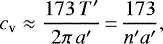
In our analytical study, we considered the planar circular restricted three-body problem (CRTBP) in the barycentric rotating reference frame where the unit of mass is the total mass of the Sun and planet (Venus in this paper), and the unit of length is the semimajor axis of the planet. When G = 1, the unit of time should be T′∕(2π), where T′ is the period of the mean motion of the planet. The numerical value of the speed of light c in the normalized unit system is denoted by cv and can be calculated by
 (7)
(7)
where a′ and n′ are the semimajor axis and mean motion of the planet, and T′ is the corresponding period in days. For Venus, cv is 8561.
The framework of an elliptic restricted three-body problem (ERTBP) in heliocentric reference frame is mainly adopted in our numerical simulations. Like the CRTBP, the ERTBP here also consists of the Sun, Venus, and a massless particle, but Venus is assumed to move in its real orbit with low eccentricity (0.00673) and inclination (3.39°) in the ecliptic system of J2000.0 centered on the Sun instead of on a circular orbit. We also considered the complete model of the current planetary configuration of our Solar System based on J2000.0 in our numerical simulations to study the effect of the planetary perturbations. All planets in the Solar System are included, and the Earth and Moon are treated as a whole body in their barycenter. All numerical simulations were carried out within the framework of the ERTBP, unless otherwise specified. Although the CRTBP is based on the barycentric reference frame, the orbital elements are always defined with respect to the Sun for all models in this paper.
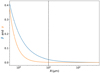 |
Fig. 1 Parameter β (blue) and γ (orange) assuming a surface potential of 10 V. The dashed line shows R = 10 μm, for which we find β = 0.0205, γ = 0.00094. |
3 Uncharged problem
The triangular Lagrangian points L4 and L5 are dynamically stable for all planets in our Solar System in the pure gravitational CRTBP (see e.g. Murray & Dermott 1999). In the vicinity of these points, an important reservoir for celestial objects such as asteroids and dust is therefore located. The investigation of these enormous populations could not only reveal the dynamical mechanisms behind the complicated orbital behavior, but also determine the possible origin of these objects and verify the scenarios proposed to describe the early stage of our Solar System.
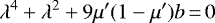
The typical phase portraits of the 1:1 MMR with Venus obtained within the framework of the ERTBP on (σ, a) and (Δω, e) planes are shown in Fig. 2. Here, σ = λ − λV is defined as the resonant angle of 1:1 MMR where λ = ω + Ω + M is the mean longitude. We note for planar CRTBP that ω and Ω have no definition so that σ = M − MV. We use Δω = ω − ωV to denote the difference in argument of perihelion between the particle and Venus, and e is the eccentricity of the dust particle. We integrated 60 orbits for each plot in the framework of the ERTBP. Two stable points in the center of tadpole regimes, which are denoted by L4 and L5, reside symmetrically at 60° and 300°, respectively. The saddle point L3, located at 180°, separates two tadpole regimes and the horseshoe regime. We note that the semimajor axis a in the plot is normalized by 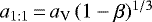 , which is the location of the 1:1 MMR for dust particles (see below). Here β = 0 and so a1:1 = aV. The apsidal difference Δω could librate around the center for orbits nearby. The center (Δωk, ek) with k = 4, 5 is (± 60°, eV) for L4 and L5. The phase portraits on the (Δω, e) plane are also symmetric for L4 and L5 when β = 0, so that we only show the portrait for the former in Fig. 2.
 |
Fig. 2 Phase portrait of the 1:1 MMR with Venus in the ERTBP. Upper panel: (σ, a) plane with resonant angle σ and (normalized) semimajor axis a, while lower panel: (Δω, e) plane (for L4 only) with apsidal difference Δω and eccentricity e. |
3.1 Location of triangular Lagrangian points
The theoretical derivation in this section is based on the planar CRTBP. We aim to derive formulae to predict the shift of the Lagrangian points L4 and L5 due to the nongravitational effects, that is, radiation pressure and the P-R-S effect. We worked in synodic coordinates where r1 and r2 indicate the position vectors from the Sun and planet, respectively. The distance to the Sun r (in Eqs. (2), (3), and (5)) therefore equals r1. In the rotating reference frame centered on the center of mass of the Sun-planet system with the planet fixed at the + x -axis, the equations of motion including Fs∕p in the planar case (Chernikov 1970; Schuerman 1980) can be written as
![Mathematical equation: \begin{equation*}\begin{array}{l@{}l@{}l} \ddot{x}&\displaystyle -2\dot{y}+\frac{\gamma_c\,(1+s_w)}{r_1^2}\left\{\dot{x}+\left[\dot{x}\,(x+\mu')+\dot{y}\,y\right] \frac{x+\mu'}{r_1^2}\right\} \\[6pt] &\displaystyle =-\frac{(1-\beta)\,\mu\,(x+\mu')}{r_1^3}-\frac{\mu'\,(x-\mu)}{r_2^3}+x+\frac{\gamma_c\,(1+s_w)\,y}{r_1^2}, \end{array} \end{equation*}](/articles/aa/full_html/2021/01/aa39617-20/aa39617-20-eq10.png) (8)
(8)
![Mathematical equation: \begin{equation*}\begin{array}{l@{}l@{}l} \ddot{y}&\displaystyle +2\dot{x}+\frac{\gamma_c\,(1+s_w)}{r_1^2}\left\{\dot{y}+\left[\dot{x}\,(x+\mu')+\dot{y}\,y\right]\frac{y}{r_1^2}\right\} \\[6pt] &\displaystyle =-\frac{(1-\beta)\,\mu\,y}{r_1^3}-\frac{\mu'\,y}{r_2^3}+y-\frac{\gamma_c\,(1+s_w)\,(x+\mu')}{r_1^2}, \end{array} \end{equation*}](/articles/aa/full_html/2021/01/aa39617-20/aa39617-20-eq11.png) (9)
(9)
where μ′ = 1 − μ is the mass of the planet, (x, y) are the coordinates of the dust particle with respect to the barycenter of the Sun and Venus, r2 indicates the distance to the planet, and γc is a parameter given by γc ≡ β μ∕c = β (1 − μ′)∕c, which mainly determines the magnitude of the P-R-S effect for particles on specific orbits (see Eq. (2)).
In addition to our analytical solutions to Eqs. (8) and (9), some numerical simulations within the framework of the ERTBP were conducted to verify the theoretical formulae. We also included other planets in the Solar System to study the effect of the planetary perturbations on the co-orbital dynamics for Venus.
3.1.1 Analytical study
When β≠0, nongravitational effects introduce additional forces that are related to the position and velocity of the particles. Therefore the equation of motion in the classic CRTBP should be modified, and the equilibrium solutions were changed accordingly. Because nongravitational effects are dependent on β, which is determined by the size of the particle, the locations of the triangular Lagrangian points rely on the size of particles.
In the rotating reference frame of the CRTBP, the locations of libration points considering solar radiation pressure and the P-R-S effect are determined by setting ẍ = ý = ẋ = ẏ = 0 in Eqs. (8) and (9). Following Schuerman (1980), we defined the following symbols:
![Mathematical equation: \begin{eqnarray}r_1^{(0)}& = &(1-\beta)^{1/3}\,{=}\,\delta,\\r_2^{(0)}& = &1,\\x^{(0)}& = &\frac{(1-\beta)^{2/3}}{2}-\mu'\,{=}\,\frac{\delta^2}{2}-\mu'\,{=}\,x_0,\\y^{(0)}& = &{\pm}(1-\beta)^{1/3}\left[1-\frac{(1-\beta)^{2/3}}{4}\right]^{1/2} \nonumber \\ & = &{\pm}\delta\left(1-\frac{\delta^2}{4}\right)^{1/2}\,{=}\,y_0, \end{eqnarray}](/articles/aa/full_html/2021/01/aa39617-20/aa39617-20-eq12.png)
which are also the analytical solution of the locations of L4 and L5 when we ignore the P-R-S effect and consider only solar radiation pressure. We note that the plus sign in Eq. (13) corresponds to L4 while the minus corresponds to L5.
We multiplied Eq. (8) by y and Eq. (9) by (x + μ′), then subtracted them. Making use of ẍ = ý = ẋ = ẏ = 0 and recalling that 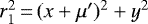 , we can obtain
![Mathematical equation: \begin{equation*}r_2\,{=}\,\left[1-\frac{\gamma_c\,(1+s_w)}{\mu'\,y}\right]^{-1/3}. \end{equation*}](/articles/aa/full_html/2021/01/aa39617-20/aa39617-20-eq14.png) (14)
(14)
To keep r2 > 0 (it is always satisfied for L5), we should ensure that for L4
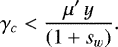 (15)
(15)
Or equivalently,
 (16)
(16)
Applying Eq. (16) to Venus and taking y ≈ y0, we can obtain β < 0.01356 for L4. Substituting the expression of r2, given by Eq. (14), in the right-hand side of Eq. (9) which is equal to 0, we obtain
![Mathematical equation: \begin{equation*}\left[\gamma_c\,(1+s_w)+(1-\mu')\,y\right]r_1^3-\gamma_c\,(1+s_w)\,(x+\mu')\,r_1\,{=}\,\delta^3\,(1-\mu')\,y. \end{equation*}](/articles/aa/full_html/2021/01/aa39617-20/aa39617-20-eq17.png) (17)
(17)
Since
 (18)
(18)
we can rewrite Eq. (17) as
![Mathematical equation: \begin{equation*}\begin{array}{ll} \hspace*{-7pt}&\displaystyle \left[\frac{\gamma_c\,(1+s_w)}{2}+(1-\mu')\,y\right]r_1^3+\frac{\gamma_c\,(1+s_w)}{2} \\[6pt] &\displaystyle \quad\times\left\{\left[1-\frac{\gamma_c\,(1+s_w)}{\mu'\,y}\right]^{-2/3}-1\right\}\,r_1\,{=}\,\delta^3\,(1-\mu')\,y. \end{array} \end{equation*}](/articles/aa/full_html/2021/01/aa39617-20/aa39617-20-eq19.png) (19)
(19)
The Nth order solution to Eqs. (19) and (14) can be written as a series expansion in γc :
![Mathematical equation: \begin{equation*}\begin{array}{ll} &\displaystyle x^{(N)}\,{=}\,\sum^N_{m\,{=}\,0}\,p^{(m)}_{4,5}(\beta,\mu')\,\gamma_c^m\,(1+s_w)^m,\\[6pt] &\displaystyle y^{(N)}\,{=}\,\sum^N_{m\,{=}\,0}\,q^{(m)}_{4,5}(\beta,\mu')\,\gamma_c^m\,(1+s_w)^m, \end{array} \end{equation*}](/articles/aa/full_html/2021/01/aa39617-20/aa39617-20-eq20.png) (20)
(20)
where  and
and  are coefficients of the mth order term for L4 or L5. Obviously
  and
and  . Solutions up to the third order are derived in Appendix A.1. Because the solutions are complicated, we tried to simplify them by assigning β = 0 in
  and
and  for m > 0 terms. Therefore, the coefficients
  and
and  with m > 0 are only dependent on μ′. This is feasible because in the case of Venus, even the original formulae shown in Appendix sectionlinking A.1 are well consistent with the numerical solutions to the equations of motion only when β ≲ 0.01 for both L4 and L5 (see below). In this region we have small differences in the resonant angles of libration centers σk (k = 4, 5) between original and simplified formulae, up to 0.12° and 0.007° for L4 and L5, respectively. Up to the third order in γc, we have
![Mathematical equation: \begin{equation*}\begin{array}{l@{}ll@{}llll} p^{(1)}_4& = &\displaystyle -p^{(1)}_5& = &&\displaystyle-\frac{2-\mu'}{3 \sqrt{3} (1-\mu')\mu},& \\[10pt] p^{(2)}_4& = &\displaystyle p^{(2)}_5& = &&\displaystyle\frac{(64-9 \mu') \mu'-44}{162 (1-\mu')^2 \mu'^2},& \\[10pt] p^{(3)}_4& = &\displaystyle -p^{(3)}_5& = &&\displaystyle\frac{u [-3 (102-\mu') \mu'+520]-248}{729 \sqrt{3} (1-\mu')^3 \mu'^3},& \\[10pt] q^{(1)}_4& = &\displaystyle q^{(1)}_5& = &&\displaystyle\frac{2-3 \mu'}{9 \mu'(1-\mu')},& \\[10pt] q^{(2)}_4& = &\displaystyle -q^{(2)}_5& = &&\displaystyle\frac{-\mu' (16 - 13 \mu')+4}{54 \sqrt{3} (1 - \mu')^2 {\mu'} ^2},& \\[10pt] q^{(3)}_4& = &\displaystyle q^{(3)}_5& = &&\displaystyle-\frac{3 \mu' [\mu' (27 \mu' -58)+16]+40}{2187 (1 - \mu')^3 {\mu'} ^3}.& \end{array} \end{equation*}](/articles/aa/full_html/2021/01/aa39617-20/aa39617-20-eq29.png) (21)
(21)
Equations (12) and (13) show that the locations of L4 and L5 are symmetric for γc = 0. The distance from both L4 and L5 to the Sun is between 0 and 1 for 0 < β < 1. As the effect of solar radiation pressure, the triangular Lagrangian points approach the Sun for increasing values of β, while the distance from the planet remains unchanged. This causes a larger resonant angle for L4 (> 60°) and a smaller resonant angle for L5 (< 300°). However, when we take the P-R-S effect into consideration, Eq. (14) tells us that L4 recedes from the planet while L5 approaches (y > 0 for L4 while y < 0 for L5). This leads to the asymmetry between L4 and L5. Therefore, the combined effect of solar radiation pressure and the P-R-S effect always drives L4 away from the planet. At the same time, we always have r1 < δ from Eq. (19) for L4. This causes the resonant angle of L4 to increase rapidly with β. The situation is much more complicated for L5. To the first order (see Eq. (A.3)), r1 is always larger than δ, however, which causes the resonant angle to increase. In this case, solar radiation pressure competes with the P-R-S effect to slow down the increase or decrease of the resonant angle, which depends on the value of parameter β and cv. We recall Eq. (7), and we find that cv is inversely proportional to vp∕c, where vp is the velocity of the planet and is close to the velocity of particles v. Therefore a larger cv corresponds to a smaller v∕c and thus a weaker P-R-S effect (see Eq. (2)). When cv is large, solar radiation pressure is more likely to dominate so that the resonant angle of L5 still decreases with β. For small enough cv, however, the P-R-S effect could counteract the effect of solar radiation pressure or even dominate the motion, leading to an increase in resonant angle.
3.1.2 Application to Venus
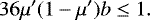
We applied our formulae to Venus. For L4 and L5, in addition to the simplified formulae shown in Eq. (21) and the original formulae (first-order to third-order solutions) shown in Appendix A.1, we can also obtain (x, y) for L4 and L5 by either numerically solving Eqs. (19) and (14) via Newton’s method (denoted by “numerical solution” hereafter) or numerically integrating the equation of motion directly (denoted by “simulation” hereafter). Then the resonant angle σk is calculated with the formulae describing the transformation from the barycentric (CRTBP) or heliocentric (ERTBP) Cartesian coordinate system to heliocentric polar coordinate system. We implemented the Newton method in a Python code to compute the numerical solutions and adopted the SyMBA integrator for simulations. In numerical simulations, the positions of libration centers (σk, ak) are determined by locating the centers of libration island in the phase portraits on the (σ, a) plane for different β, where the libration amplitudes Δσ (max[σ] −min[σ]) are minimum. Concretely, we sampled hundreds of orbits with initial conditions on the (σ0, a0) plane for each β and then integrated them for thousands of years. The other orbital elements were set to be the same as those of Venus. The intervals of β were set to be 10−4 and 0.002 for L4 and L5, respectively. Then we delimited the region of libration centers by comparing the libration amplitudes of these orbits. Afterward, the region enclosing the orbits with minimum libration amplitudes was located. Iteratively, we were able to sample and integrate some orbits in this reduced region and repeated the above steps until we reached a desired resolution. Because there is almost no difference in value between ak and a1:1, we always used a1:1 to evaluate ak for simplicity.
The resonant angles for different Lagrangian points σk from various solutions are shown in Fig. 3. Apparently, σ4 and σ5 always increase with β. The numerical solutions to Eqs. (19) and (14) agree perfectly with the result of numerical simulations based on the ERTBP. Both of them show that there are no solutions for β > 0.01135 for L4 and β > 0.33865 for L5 because they have collided with L3 and L1, respectively (see below). However, even the third-order approximation formula cannot determine the real libration center for large β, especially for L5. Intuitively, this is because the parameter cv (≈ 8561) in this case is not large enough, leading to a relatively large γc and slow convergence of the expansion. In other words, the high orbital velocity of Venus results in a relatively large v∕c, which corresponds to a relatively small cv according to Eq. (7). This means that it is not very effective to treat the perturbation from the P-R-S effect as an expansion in γc for large β. At the same time, small cv could also cause an increase of the resonant angle of L5 because the P-R-S effect is more effective here, as we mentioned before.
Given corresponding initial positions (x, y), we can also numerically solve Eqs. (19) and (14) via Newton’s method and then calculate the resonant angle for L1, L2, and L3. As shown in Fig. 3, σ1 and σ3 decrease with β. Finally, L3 coincides with L4 at β = 0.01135 with σ3 = σ4 = 108.4°. Similarly, L1 coincides with L5 at β = 0.33865 with σ1 = σ5 = −5.57°. For larger β, these Lagrangian points disappear and the corresponding equilibrium solutions no longer exist. L2 is always located in the forth quadrant forany nonzero β and σ2 varies in an extremely small range (<5 × 10⁻⁵ deg for 0 < β < 1).
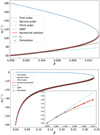 |
Fig. 3 Resonant angle of the libration centers (σk) for L4 (top) and L5 (bottom) of Venus from different solutions. The positions of the libration centers for L3 and L1 obtained from the numerical solutions to the equations of motion are also presented in the upper and lower panels, respectively. “SIMP” represents the results calculated from the simplified approximation formulae Eqs. (20) and (21). The results from approximation formulae for L5 are only shown for 0 < β < 0.01 (we insert a window to zoom in) because their deviations from the numerical solutions are too large for β > 0.01. |
3.2 Linear stability
Consider a dust particle that is given a small displacement (X, Y) from the equilibrium point (X0, Y0). The linearized equations of motion (see Appendix A.2) have the form
 (22)
(22)
where A is the matrix (aij), with aij (i, j = 0...3) indicating the linear coefficients with respect to X, Y, Ẋ, and Ẏ in Eqs. (A.15), (A.16), and
 (23)
(23)
The characteristic equation of A can be written as
 (24)
(24)
where ak (k = 0...3) are expressions obtained from aij and
 (25)
(25)
Neglecting the P-R-S effect, that is, setting γc = 0, we have ai (i = 0...3) = 0. Then Eq. (24) becomes
 (26)
(26)
with the solutions
![Mathematical equation: \begin{equation*}\lambda_0\,{=}\,{\pm}\mathrm{i}\left\{\frac{1}{2}{\pm}\left[\frac{1}{4}-9\mu'(1-\mu')b\right]^{1/2}\right\}^{1/2}\,{=}\,\mathrm{i}\,\lambda_r. \end{equation*}](/articles/aa/full_html/2021/01/aa39617-20/aa39617-20-eq35.png) (27)
(27)
In the absence of nongravitational effects except for solar radiation pressure, L4 and L5 are stable if
 (28)
(28)
This constraint is satisfied for all b in (0, 1) when
 (29)
(29)
In the presence of the P-R-S effect, we can also solve Eq. (24) by expanding the parameters ak in γc. The second-order solution is presented in Appendix A.2. We note that there always exists a positive real part for λ when γc > 0, which means that L4 and L5 are unstable when we consider the P-R-S effect.
Taking μ′≈ 0, the e-folding time of dust particles, which is the time interval in which the oscillation around the Lagrangian points increases by a factor of e, can be given by
 (30)
(30)
The first-order term in γc has been derived in Schuerman (1980), and we developed it to the second order. The second-order term is opposite for L4 and L5 because they have opposite y0. Therefore the e-folding time for L4 is slightly longer than that for L5. We also extended the solution to the third order. However, μ′ = 0 is a singularity for the third-order solution, so that we cannot give a similar simplified formula for the e-folding time. The linear stability analysis suggests that the stability of triangular Lagrangian points, which is reflected by the e-folding time, declines with β. This qualitative result can be confirmed by numerical simulations. Quantitatively, however, the e-folding time is not necessarily equivalent to the lifespan of particles, which is the time duration of staying in the 1:1 MMR region because the linear stability analysis is conducted in a small neighborhood around the equilibrium point. For Venus, the lifespans are much longer than the e-folding time (see Sect. 3.3).
In Fig. 4 we present an example describing the orbital evolution of a particle in L5 with β = 0.07. The initial conditions were set to be in the libration center (ak, ek, iV, Δωk, ΩV, σk) = (0.706 AU, 0.0064, 3.39°, −38.45°, 76.68°, −25.93°) in the ERTBP (see Sec. 3.3). The orbit librated around the libration center with extremely small amplitudes at the beginning. After about 30 kyr, the variations in semimajor axis and resonant angle started to increase. Then the eccentricity changed dramatically, and finally, the orbit escaped at about 45 kyr. As mentioned in Lhotka & Gales (2019), the inclination and longitude of ascending node stay more or less unchanged in the uncharged problem before the orbits escape from the co-orbital region. According to Eq. (30), the e-folding time is about 3 kyr for β = 0.07 for L5. It is much shorter than the lifespan (45 kyr), as we mentioned before.
3.3 Numerical study. ERTBP and N-body
To better illustrate how solar radiation pressure and P-R-S effect affect the dynamical behavior of orbits in 1:1 MMR, we constructed the phase portraits for different values of β on the (σ, a) plane. Figure 5 presents a comparison between β = 0.006 and β = 0.012. Sixty orbits initially equally spaced (Δσ0 = 6°) along a = a1:1 were integrated for 10 kyr for each plot within the framework of the ERTBP. The typical phase portrait on the (σ, a) plane without any nongravitational effect is shown in Fig. 2, where the locations of L4 and L5 are symmetric and L3 is located at 180°. However, the presence of β brings in an asymmetry to the phase portrait. There exists a displacement of L3, L4 and L5 for 0 < β < 0.01135, as the example of β = 0.006 shows. The value of σ corresponding to L3 decreases to 153.7°, while L4 (72.8°) and L5 (308.0°) shift to the right. These data are obtained from numerical simulations (L4 and L5) and numerical solutions to the equations of motion (L3). Apparently, they perfectly depict the locations of libration points and saddles in the phase portraits (indicated by vertical lines). The perturbation caused by the P-R-S effect gives rise to chaos because the dispersion of orbits in the phase portraits is visible, especially for those far away from triangular Lagrangian points. As mentioned in Sect. 3.1, for β > 0.01135, L3 and L4 merge and disappear. Along with this, the tadpole region of L4 vanishes. This is clearly shown by the example of β = 0.012, in which the value of σ for L5 is 313.6°. For all β, the positions of equilibrium points on the a axis are very close to a1:1.
In Sect. 3.1 we have also shown a good agreement between the results from the analysis of the CRTBP and numerical simulations in the ERTBP (see Fig. 3) only with a slight difference between them (denoted by Δσk) that is due to the eccentricity of Venus. We calculated the difference in σk between the numerical solutions (in the CRTBP) and simulations (in the ERTBP). Figure 6 shows that σk in the CRTBP is always larger than that in the ERTBP, and this kind of difference increases with β generally. The eccentricity of Venus has a larger effect for L4 (up to 0.13°) than L5 (up to 0.025°). We also note smooth trends of Δσk versus β, especially for small β. We assume that an expansion similar to that in Sect. 3.1 could be conducted to solve the equations of motion within the framework of the ERTBP. Some additional term involved with β should appear due to the eccentricity of Venus.
We onlyconsidered the case of three-body problem so far. For 1:1 MMR with Venus, the perturbation from the other planets in the Solar System could play an important role in the dynamical evolution of dust orbits. In our paper about Venus (Trojans, in prep.), we conduct a comprehensive investigation of the resonance mechanism in the complete model that includes all planets of the Solar System. In Fig. 6 we also present the deviations in σk between thecomplete model and ERTBP. In contrast to the CRTBP, the planetary perturbations giving rise to the onset of chaos in the whole vicinity of the equilibrium points cause disordered deviations to σk. However, the planetary perturbations result in a comparable shift Δσk as the CRTBP.
As revealed by Fig. 5, in addition to the resonant angle of libration centers σk, the libration width of tadpole regions (δa) also varies with β. Obviously, the tadpole region of L4 decreases with increasing values of β until it disappears completely. In contrast, thetadpole cloud of L5 expands with β. In practice, we classified the orbits starting in the vicinity of L4 that never exceedL3 during the integration into the tadpole region of L4. Similarly, the tadpole region of L5 consists of the orbits starting in the vicinity of L5 that never go below L3. Many orbitswere integrated to precisely delimit the boundary of the tadpole region. In our simulations we used the values of σ for L3 obtained from the numerical solutions to the equations of motion (blue curve in the top panel of Fig. 3) in order to classify the tadpole regions of L4 and L5. As we mentioned in Sect. 3.1, L3 and L4 coincide and disappear for β > 0.01135. In this case, we can no longer define the above-mentioned libration width. Finally, the libration width of each triangular Lagrangian point is defined as the maximum difference in semimajor axis of the orbits belonging to the corresponding tadpole region.
According to Murray & Dermott (1999), massless particles are thought to move on tadpole orbits if  , where δr is the radial separation of particles from Venus. This condition holds for both L4 and L5 if β = 0, as shown in Fig. 7. This figure also shows that the libration width of L4 decreases with β, while the width of L5 increases with β. The corrections are almost linear, especially for L5, where the slope is lower (0.158 v.s. − 0.184 by linear fitting). The libration width of L4 decreases to zero at β = 0.01135 and the tadpole region around L4 vanishes. At the same time, δa of L5 increases to 4.360 × 10⁻³ aV.
The planetary perturbations could affect the size of tadpole regions by both changing the location of L3 and affecting the dynamical behavior near the boundary of tadpole regions. The difference is unremarkable in most cases, however. The maximum deviation is less than 5 × 10⁻⁷ aV. Considering that the libration width tends to 0 for L4 when β tends to 0.01135, however, the planetary perturbations play an increasingly important role with increasing values of β.
When we include the horseshoe orbits, determining the extended libration width of the 1:1 MMR region (Δa) becomes more complicated because such orbits are chaotic due to the P-R-S effect. We set different criteria to describe the boundary of the 1:1 MMR region of Venus. Three different thresholds (340°, 350°, and 353°) indicating the maximum allowed libration amplitudes were chosen. The results shown in Fig. 8 suggest that the libration width of the 1:1 MMR increases with β first and then decreases. It is obvious that a higher threshold value of libration amplitudes produces a smaller turning point. In the region before the turning point, the libration width is heavily dependent on the threshold. This is due to the chaotic nature near the boundary, which also causes the roughness of the curve for a high threshold such as 353°. Meantime, the gradual rise of the width is caused by the expansion of the stable region around L5 (see Fig. 5). After the turning point, the increasing perturbation due to the P-R-S effect gradually destabilizes the orbits in the 1:1 MMR region. Only the particles closely orbiting L5 could survive, so the dependence of the libration width on the threshold is much weaker.
After we determined the positions of libration centers (σk, ak), we studied the change in the phase plane (Δω, e) by modifying the value of β. In Fig. 9 we show on the (Δω, e) plane the evolution of 60 orbits with initial conditions σ = σk, a = ak. According to Lhotka & Celletti (2015) and Lhotka & Gales (2019), (i, Ω) of L4 and L5 are always located at (iV, ΩV). These two elements remain unchanged during the integration and are not affected by solar radiation pressure and the P-R-S effect. In comparison with the typical phase portrait shown in Fig. 2 for β = 0, solar radiation pressure and the P-R-S effect exert additional forces in the orbital plane on dust particles and cause a deviation of the center (Δωk, ek). In addition, the orbits evolve spirally toward the center in the phase space regardless of the initial conditions. In the two cases we show in Fig. 9 (β = 0.004 for L4 and β = 0.05 for L5), the apsidal difference between the libration centers and Venus Δωk approaches 0 and the eccentricity ek gets lower than eV in comparison with the case of β = 0, where Δωk = ±60° and ek = eV.
Following the method we used to determine (σk, ak) in Sect. 3.1, the centers of (Δω, e) were also precisely determined by minimizing the libration amplitudes in an iterative way. Figure 10 presents the result. For β = 0, the phase portrait is symmetric for L4 and L5 and the center (Δωk, ek), where the amplitudes of e and Δω are minimum, is located at the point of (eV, ±60°). In the presence of a non-zero β, we find an asymmetry between L4 and L5. The eccentricity ek with the smallest amplitudes monotonously decreases with β for L4, at a much faster rate than for L5 in the same range of β ∈ (0, 0.01135). Therefore a maximum β value of 0.01135 corresponds to a minimum ek of 0.00235. For dust particles around L5, although ek could increase with β for 0.03< β < 0.245, it is still smaller than eV in the whole range to be considered (0, 0.33865). In short, the combined effect of solar radiation pressure and the P-R-S effect always tends to reduce the eccentricity of dust particles of any size we considered in the triangular Lagrangian points. Despite a wider range of β, ek of dust particles in L5 varies in a narrower range with a minimum value of 0.00630.
Figure 10 shows that the apsidal difference Δωk varies with β in a more sophisticated way than σk does (cf. Fig. 3). It always decreases first and then increases with β (for L5 it even decreases again for β > 0.32). The (first) turning point is β ≈ 0.008 for L4 and β ≈ 0.005 for L5. We note that it is possible to observe dust particles of specific sizes moving on orbits with Δωk = ±60°, just like the case where β = 0, but ek < eV. For L4, this size is 21 μm, corresponding to a β of 0.009963, and it is 28 μm (β = 0.00734) for L5.
Although the tadpole region of L5 and the 1:1 MMR region may be enlarged under some conditions (see Figs. 7 and 8), the stability of triangular Lagrangian points is thought to be reduced for increasing β. To verify this, we integrated the orbits in the libration centers (ak, ek, iV, Δωk, ΩV, and σk) for different β. The integration of one particle was ended when it escaped the 1:1 MMR region of Venus, and then we recorded the lifespan. After several test simulations, we applied a criterion that if an orbit dissatisfies |a −ak| < 0.0075 AU at any time, it was regarded as escaped. It is feasible to set a threshold of 0.0075 AU, which is slightly higher than the maximum half-width of the 1:1 MMR region (see Fig. 8), because the orbits escaping the 1:1 MMR are scattered away or fall into the star in a short time. Generally, the lifespans shown in Fig. 11 decrease with β, indicating a diminishing stability. The trends of lifespans for L4 and L5 seem to be similar in the range of β < 0.01135. In the CRTBP, the triangular Lagrangian points are dynamically stable for all planets of the Solar System. When we included solar radiation pressure and the P-R-S effect, L4 and L5 were no longer stable. This was shown in the linear stability analysis in Sect. 3.2. As we also mentioned there, the lifespans here are several times longer than the e-folding time, but these two time scales follow a similar trend with β. Figure 11 also shows that the lifespan is about 38 Myr for orbits in L4 with β = 10−4 and about 1.8 Myr for orbits in L5 with β = 0.002. As β increases, the lifespan drops monotonously in general and decreases to 0.1 Myr when β = 0.03 (only for L5).
 |
Fig. 4 Orbital evolution of particles in L5 with β = 0.07 (R = 2.9 μm) based on the ERTBP. The orbit is initially placed in the libration center (see more details in the text). |
 |
Fig. 5 Phase portrait on the (σ, a) plane. Upperpanel: obtained for β = 0.006, while lower panel: obtained for β = 0.012. The vertical lines indicate σk obtained from numerical simulations (L4 and L5) and numerical solutions to the equations of motion (L3), which are 72.8° (L4), 153.7° (L3) and 308.0° (L5) for β = 0.006, 313.6° (L5) for β = 0.012. |
 |
Fig. 6 Difference of resonant angles of libration centers (Δσk) between different models and the ERTBP for L4 (top) and L5 (bottom). “pp” means the planetary perturbations. |
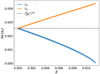 |
Fig. 7 Libration width of tadpole regions for L4 (blue) and L5 (orange). The dashed line represents the result from the theoretical formula for β = 0. The interval of β for L5 is set to be the same as that of L4 in this case (10−4). |
 |
Fig. 8 Libration width of 1:1 MMR with Venus for different thresholds. See text for more details. |
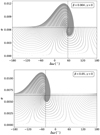 |
Fig. 9 Phase portrait on the (Δω, e) plane. Upperpanel: β = 0.004 for L4, and lower panel: β = 0.05 for L5. The horizontal and vertical lines indicate ek and Δωk obtained by minimizing the libration amplitudes, which are 0.00644 and 55.90° for the upperpanel, 0.006355 and − 43.24° for the lower panel. |
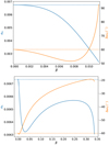 |
Fig. 10 Eccentricity (blue) and apsidal difference (orange) with the smallest amplitudes for different values of β for L4 (top) and L5 (bottom). The blue horizontal line indicates the eccentricity of Venus (0.00673), and the orange horizontal line indicates ± 60°. |
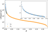 |
Fig. 11 Lifespans of dust particles in the libration centers of L4 and L5. A window is inserted to zoom in the region of 0 < β < 0.012. |
4 Charged problem
In this section we reexamine the results of the previous section including the charge, that is, we focus on the role of the interplanetary magnetic field on captured charged dust grains in co-orbital resonance with Venus. Given the background magnetic field strength at specific distance, solar rotation rate and solar wind speed (see Table. 1), the Lorentz force shown in Eq. (5) is determined by the charge-to-mass ratio, position, velocity, and the deviation of the magnetic and orbital angular momentum axis.
4.1 Shift of resonance and capture time
In consideration of the important effect of the interplanetary magnetic field, especially for small particles (see e.g. Mann et al. 2014; Lhotka & Gales, 2019), we introduced the Lorentz force in our simulations. The charge-to-mass ratio q∕m (or γ) is related to β through Eq. (6), which can be written as γ ≈ 0.224 Uβ2 assuming ρ = 2.8 g cm−3. We adopted the value of the maximum surface potential (U = 10 V) used in Mann et al. (2014) and Lhotka & Gales (2019) in this section, and thus we have γ ≈ 2.24 β2.
A comparison of the orbital evolution between charged and uncharged particles is shown in Fig. 12. We switched on the Lorentz force for the orbit shown in Fig. 4. The corresponding value of γ is 0.011 for β = 0.07. We observe a shorter lifespan for the charged particle (~30 kyr). Except for this, however, the semimajor axis and resonant angle have a similar evolution for both particles, although the Lorentz force causes larger libration amplitudes at the very beginning. A close inspection also suggests that under the effect of the Lorentz force, deviations in the locations of libration centers in the phase space exist, especially in e and Δω. Furthermore, i and Ω are no longer constant during the integration because of the additional normal force exerted by the interplanetary magnetic field. The inclination can be pumped up to ~10°. The longitude of the ascending node follows a similar evolution as the inclination, librating with decreasing amplitudes. i and Ω are coupled, and their variation is confirmed to be related to the deviation of the magnetic axis from the angular momentum axis of the system, the initial inclination, and the ratio Ωs∕n (Lhotka et al. 2016; Lhotka & Gales, 2019).
The resonant angle of libration centers σk depends on the Lorentz force. Because we fixed the surface potential, the Lorentz force is larger for smaller particles, whose β are also larger, according to γ ≈ 2.24 β2. We repeated the iterative method in Sect. 3.1 to locate σk of libration centers. The upper panel of Fig. 13 shows that for L4 the Lorentz force has a negligible effect on σk for β < 0.0085, corresponding to R > 24 μm and γ < 1.6 × 10⁻⁴. Even a higher value of γ can only cause a deviation nogreater than 0.02° in σ4. This is principally due to the low limit of β (≤ 0.01135) required by the existence of L4 (see Sect. 3.1), which corresponds to a small limit of γ (≤ 2.9 × 10⁻⁴) and thus a small Lorentz force. However, when a higher value of β is allowed, as in the case of L5 where β ≤0.33865, the Lorentz force could become larger and affect the position of L5 in a more effective way (see the lower panel of Fig. 13). The maximum difference Δσk could reach 2.4°, which corresponds to a distance of 4.5 × 10⁶ km from the location of the exact libration point in uncharged problem. In addition, for β >0.276, no stable points can be found in the phase portrait because of the chaos that is induced by the interplanetary magnetic field, which also causes the chaotic variation in Δσk with γ. Figure 13 also shows that in general, σk in the charged problem seems to be smaller than that in the uncharged problem for L4 (negative Δσ4) and larger than that in the uncharged problem for L5 (positive Δσ5) for most β.
Planetary perturbations might clearly enhance the chaotic behavior in the whole system. The isolated effect of the Lorentz force on the position of L4 (see Fig. 13) is slightly smaller than that of planetary perturbations (see also Fig. 6). However, for L5, of which the β range is much wider, the deviation coming from planetary perturbations is negligible in comparison of that from the Lorentz force for β > 0.054 (see the lower panel of Fig. 13). We also took into account the planetary perturbations and Lorentz force in our simulations. When these two forces are comparable in magnitude, the combined effect may produce a larger deviation in σk, just like in the case of L4 (see the top panel in Fig. 13). However, when one of these two forces dominates, the combined effect follows the dominant effect, just like in the case of L5 (see the lower panel in Fig. 13).
The Lorentz force could further enlarge the tadpole region of L5 while reducing the tadpole region of L4 (not shown here). In comparison with a maximum deviation of 3.5 × 10⁻⁷ aV in the libration width of L5, the Lorentz force has a much stronger effect on the tadpole region in L4, which can be reduced by up to 8 × 10⁻⁶ aV. Although the deviations are very small, this reduction could be really remarkable (up to 15%) because the libration width of L4 for uncharged particles is also very small for large β.
We show in Fig. 14 the apsidal difference from Venus (Δωk) and the eccentricity (ek) of the libration centers in a charged problem (shown in dots) obtained with the same method mentioned in Sect. 3.3. Apparently, they differ from the results in the uncharged problem (shown in curves) under the effect of the Lorentz force. We conclude that the Lorentz force tends to increase Δωk but decreases ek for both L4 and L5 in most situations. For L4, γ is limited to 3 × 10⁻⁴ due to the maximum value of β 0.01135. Therefore the perturbation from the interplanetary field is small enough for us to determine (Δωk, ek) precisely. Conversely, the orbits inL5 with β > 0.05 are much more chaotic. The lifespans of such orbits are reduced, and the libration centers cannot be located precisely, especially for β > 0.244, for which (Δωk, ek) cannot be determined because the lifespans are too short. However, we can still demonstrate that the Lorentz force can greatly change ek and Δωk. The maximum differences could be up to 0.0022 and 25° for ek and Δωk, respectively.
Because many secular resonances control the dynamical behavior of particles in 1:1 MMR with Venus, the eccentricity and apsidal difference could experience complicated secular evolution. We therefore not show the plot of (Δωk, ek) under the effect of the planetary perturbations.
The lifespans of charged particles in the libration centers shown in Fig. 15 again confirm that the perturbation from the interplanetary magnetic field further destabilizes the co-orbital region. Considering the uncertainties in determining the lifespans, we find a significant decrease in lifespans for β >0.0105 for both L4 and L5. The lifespan difference is about 105 yr for β = 0.01135, although the Lorentz force is smaller for smaller γ, but the longer lifespan makes it easier to accumulate the effect. On the other hand, the Lorentz force can also significantly reduce the stability within the short lifespan of large dust particles. The planetary perturbations can only cause a very limited difference to the lifespans compared to the Lorentz force. The most important dynamical effects caused by other planets on the co-orbital region are secular resonances (see, e.g., Brasser & Lehto 2002; Zhou et al. 2009, 2011, 2019, 2020; Dvorak et al. 2012), which need a long timescale to be effective. Before this, however, dust particles are very likely to have escaped from the 1:1 MMR as a result of nongravitational effects.
 |
Fig. 12 Orbital evolution of particles initially located in L5 for β = 0.07. Orange curves indicate the model including the Lorentz force with γ = 0.011 (surface potential = 10 V), and the blue curves indicate the same orbit as in Fig. 4, where γ = 0. Both orbits are initially placed in the libration center of the uncharged problem. |
 |
Fig. 13 Differences of resonant angles of libration centers Δσk between different models and the ERTBP for L4 (top) and L5 (bottom). “Charged” refers to the model including the Lorentz force. |
 |
Fig. 14 Same as Fig. 10, but dots indicate the model including the Lorentz force given a surface potential of 10 V. |
4.2 Parameter space study
In this section we investigate the effect of charge on the full parameter space (β, γ) with 0 ≤ β ≤ 0.01135 for L4 and 0 ≤ β ≤ 0.33865 for L5 and γ derived from Eq. (6), with 0 ≤ U ≤ 10 Volt (for L4 and L5) with the aim to provide the domain in β × γ for which charge cannot be neglected in dynamical studies of dust in the Solar System. The results are based on the ERTBP with the standard Parker model for the interplanetary magnetic field. The initial conditions for the numerical simulations are as follows: for fixed pairs of parameters (β, γ), we chose initial conditions centered at the equilibria of L4 and L5, taken from our previous analysis, together with initial conditions with slight deviations of δa = ±10−3 (normalized units), δσ = ±1°, δΔω = ±1°, or δe = ±ek (with equilibrium value ek for L4 and L5, respectively). This gives nine initial conditions in total for each pair (β, γ), but this is sufficient to investigate the effect of the charge parameter γ on (i) the time of temporary capture and (ii) the maximum libration amplitudes compared to the uncharged case defined with γ = 0. Let Tγ be the time of temporary capture for a fixed pair of values (β, γ) normalized by the time of temporary capture for the same β, but with γ = 0.
The results for the case L5 are shown in Fig. 16, where we report the value of Tγ with 0 ≤ Tγ ≤ 1 in the parameter space (β, γ). As expected, for lower values of γ, we find Tγ > 0.5 up to β≃ 0.3 with Tγ close to one for small β and decreasing with increasing β. We also provide test cases within the green region in Fig. 17 with three orbits each for values (β, γ) in the dark green region (a), the light green region (b), and in the white region (c). We note that even low values of γ are sufficient to obtain Tγ ≃ 0 for β >0.3. With increasing values of γ, we find decreasing Tγ for the full range of β ≤ 0.3 up to the threshold γ ≃ 0.01 where Tγ < 0.5. Within the light red regime of Fig. 16 we still find capture, with much shorter capture times, while in the dark red regions the perturbations due to charge dominate the other effects. For comparison we also provide orbits within the red regions (d, e) in Fig. 17. We clearly see the reduction of the capture time caused by charge and perturbations of the interplanetary magnetic field. We conclude that the effects of the interplanetary magnetic field further destabilize motion in 1:1 resonance with Venus compared with vanishing charge-to-mass ratios in case of L5.
The situation is somewhat different for the leading Lagrange point L4. Already the standard nongravitational effect, that is, the P-R-S effect, destabilizes the orbits of captured dust in the uncharged case, and no capture persists for values with β > 0.01135. For surface potentials U ≤ 10 V the effect of γ is therefore not sufficiently large to act on the dynamics, that is, the capture processes. A similar study in the case of L4 reveals that in the full parameter space (β, γ), we find Tγ ≃ 1 for all parameters and initial conditions (however, charge, i.e., the effect of the interplanetary magnetic field, still affects the maximum libration width; this is not shown here).
 |
Fig. 15 Lifespans of dust particles in the libration centers of L4 and L5 in the charged problem. A window is inserted to zoom in the region of 0 < β < 0.012. The gray dots indicate the lifespans in the uncharged problem that we showed in Fig. 11. |
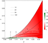 |
Fig. 16 Effect of charge-to-mass ratio γ on stability (i.e., capture) time Tγ in the parameter space (β × γ). |
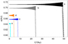 |
Fig. 17 Effect of different charge-to-mass ratios on the stability time Tγ. Parameters for orbits a–e are taken from Fig. 16 with initial conditions at the libration point L5. |
5 Summary and conclusions
We investigated the role of nongravitational effects on the dynamics of charged micron-sized dust grains in the co-orbital region of Venus. Our study includes the investigation of planetary perturbations, solar radiation pressure, the Poynting-Robertson effect, and solar wind drag (P-R-S effect). In addition, we performed a detailed study of the effect of the Lorentz force as a result of theinteraction with the interplanetary magnetic field (Parker spiral model), which is usually neglected in this type of studies (e.g., Beauge & Ferraz-Mello 1994; Liou & Zook 1995; Jeong & Ishiguro 2012; Lhotka & Celletti 2015).
Our results are based on analytical estimates in the framework of simplified dynamical models, that is, the circular restricted three-body problem, and numerical studies in the elliptic restricted three-body problem, and the planetary problem including all nongravitational perturbations. We used a Fortran code that has been used in Lhotka & Gales (2019) as well as SyMBA (Duncan et al. 1998; Levison & Duncan 2000), which we modified to include the additional perturbations, that is, the Lorentz force term.
We mainly focused on studying the position of the triangular Lagrange points L3 (collinear), L4 (leading), and L5 (trailing) that define the geometry of the co-orbital regime of motions. We provided a detailed analysis of (i) the shift of the Lagrange points and (ii) the time of temporary capture of charged and uncharged dust grains in the co-orbital regime of motions, both due to the nongravitational effects. The shift and capture time strongly depend on the area-to-mass ratio of the dust grains, parameterized by the parameter β and the charge-to-mass ratio q∕m parameterized by the parameter γ.
As expected, we find that in the uncharged problem (γ = 0), the shift due to solar radiation pressure is symmetric with respect to L4 and L5, while the P-R-S effect acts asymmetrically on the location of L4 and L5. This phenomenon has previously been investigated in case of Jupiter (Lhotka & Celletti 2015). We derived an analytical formula to predict the shift for uncharged dust grains, based on the circular restricted three-body problem following the line of argumentation in Schuerman (1980). We generalized the results to higher orders in the small parameters and also performed a linear stability analysis that provides an order-of-magnitude estimate of the e-folding time. We confirmed that the nongravitational effects render the equilibria unstable.
These results serve as the basis for finding good parameters and initial conditions for massive numerical simulations in the framework of the inclined elliptic restricted three-body problem and the full planetary problem. The aim is to find orbits with minimum libration amplitudes close to L4 and L5 that define the geometry of the co-orbital regime of motion also in these more realistic dynamical models. Denoting by ak, σk, ek, and Δωk, with k = 4, 5 the semimajor axes, resonant angle, orbital eccentricity, and difference in argument of perihelion (with respect to Venus) with minimum libration amplitudes, close to the triangular Lagrange points, we provided their dependence on β as well as γ≠0. We find that nongravitational perturbations destroy librational orbits in the vicinity of L4 already at β ≃0.01135 (collision of L3 with L4), while librational orbits survive close to L5 up to β ≃ 0.33865 (collision of L1 with L5). This difference, caused by the P-R-S effect, results in an asymmetry in the shift of L4 and L5 (with respect to the pure gravitational problem) and in different extensions of the regimes of librational motion of dust close to L4 and L5. The tadpole region expands with β for L5 almost linearly, but for L4 it shrinks. For the width of the co-orbital region, which also contains the horseshoe orbits, we can always find some turning point (β ~ 0.07) where the width is the largest.
The interaction of charged dust particles (γ≠0) with the interplanetary magnetic field contributes to the shift of the tadpole points as well, but to a much lesser extent. However, for large enough γ, we also finda notable effect that is comparable to the effect of the planetary perturbations in the uncharged case. The role of charge is also more important for the trailing Lagrange point L5 that ensures librational motion up to much higher values in β that correspond to much smaller particles with much higher charge-to-mass ratios for fixed values of density and surface potential. The Lorentz force therefore also affects the libration points in the co-orbital regime of motions in an asymmetric way, supporting librational motion of tiny dust grains close to L5. Even more importantly, the Lorentz force term will act on the orbital planes of motions. In the uncharged problem, the dust grains stay within the orbital plane of Venus, neglecting the additional perturbations of the planets. However, the normal force component due to the Lorentz force will bring the dust particles out of their initial plane with latitudinal libration amplitudes up to several degrees already in the circular restricted problem. This phenomenon has been studied in full detail in Lhotka & Gales (2019) and is related to the deviation of the magnetic axis of the sun from the axis of orbital angular momentum. Deviations from the orbital plane of Venus may reach several degrees. An additional important effect of the interplanetary magnetic field is the strong effect on the capture time of particles in the co-orbital regime of Venus.
It is commonly accepted that the orbital lifespan of (uncharged) dust grains in the Solar System is limited by the Poynting-Robertson effect. Outside of MMR with the planets, the effect leads to circularization and shrinking in semimajor axes, bringing the dust grains toward the Sun on spiral-like motions (Burns et al. 1979). However, the net effect that leads to the decrease in semimajor axis can vanish in presence of outer and co-orbital resonance with a planet, with the result of temporary capture of dust at specific distances from the Sun. This capture may strongly extend the lifespan of dust grains in the Solar System. In a detailed study of time of temporary captures of charged and uncharged dust grains in the co-orbital regime with Venus, we find a strong dependence on the area-to-mass ratio, related to parameter β, that is already known. However, we also see a strong dependence of the capture time on the parameter γ; the charge-to-mass ratio of the dust particle as well. The reason is found in the faster increase of the libration amplitudes of charged dust in comparison to uncharged one. While for 0 ≤ β ≤ 0.3 the capture time (in the vicinity of L5) is about the same for γ = 0 and γ ≤ 0.01, even low values of γ≠0 may lead to release from co-orbital resonance at very short times. For higher charge-to-mass ratios γ > 0.01 the time of temporary capture may be reduced by a factor 2–10 depending on the actual value of γ. Finally, we find that the effect of the interplanetary magnetic field on capture times close to L4 and L5 is asymmetric as well; it is much more important in the vicinity of L5.
We remark that our study is based on a simplified model of the interplanetary magnetic field and assuming time-independent (equilibrium) charge-to-mass ratios of the dust grains. This is an oversimplification of the real situation in our Solar System. Time-dependent effects on the polarity and magnitude of the interplanetary magnetic field and the role of local perturbations due to coronal mass ejections have not been investigated in the present study at all. Time-dependent charge due to changes in the local plasma environment in space may result in additional effects that we have not touched on either.
However, the motivation of this study was to provide details on the role of the mean interplanetary magnetic field on the dynamics that is usually neglected by other authors. It may also serve as a basis for future studies that include more realistic models of the heliosphere. To conclude, the role of charge and the interplanetary magnetic field on the orbital motion of dust in the Solar System has been shown to be important to better understand the distribution and timescales of dust in our Solar System.
Acknowledgements
This work has been supported by the Austrian Science Fund (FWF) in the framework of the stand alone project P30542, National Natural Science Foundation of China (NSFC, Grants No. 11473016, No. 11933001) and National Key R&D Program of China (2019YFA0706601). L.Z. acknowledges the financial support from the program of China Scholarship Council (No. 201906190106) for his visit in University of Vienna.
Appendix A: Locationshift of co-orbital resonances in the Solar System
A.1 Locationof triangular Lagrangian points
To the first order in γc, Eqs. (19) and (14) can be simplified as
![Mathematical equation: \begin{equation*}\left[\frac{\gamma_c\,(1+s_w)}{2}+(1-\mu')\,y\right]r_1^3\,{=}\,\delta^3\,(1-\mu')\,y, \end{equation*}](/articles/aa/full_html/2021/01/aa39617-20/aa39617-20-eq40.png) (A.1)
(A.1)
 (A.2)
(A.2)
Assuming that  where ϵ is the coefficient of the first-order term in γc, we can obtain r1 and r2 in the form
![Mathematical equation: \begin{eqnarray}r_1^{(1)}& = &\delta\,\left[1-\frac{\gamma_c\,(1+s_w)}{6\,(1-\mu')\,y_0}\right],\\r_2^{(1)}& = &1+\frac{\gamma_c\,(1+s_w)}{3\,\mu'\,y_0}. \end{eqnarray}](/articles/aa/full_html/2021/01/aa39617-20/aa39617-20-eq43.png)
Substituting r1 and r2 with Eqs. (A.3) and (A.4) in Eq. (18), we obtain
![Mathematical equation: \begin{equation*}x^{(1)}\,{=}\,x_0\,\left[1-\frac{(1-\mu')+\mu'\,\delta^2/2}{3\,(1-\mu')\,\mu'\,x_0\,y_0}(1+s_w)\,\gamma_c\right]. \end{equation*}](/articles/aa/full_html/2021/01/aa39617-20/aa39617-20-eq44.png) (A.5)
(A.5)
We note that Eq. (A.5) is a corrected version of Eq. (19) in Schuerman (1980), and the first equation in Eq. (4) of Liou & Zook (1995) because both of them missed (1 − μ′), which is the mass fraction of the star, in the denominator. This only causes a negligible difference because the planet mass is far lower than the stellar mass, however, and thus (1 − μ′) ≈ 1. Recalling  and making use of Eqs. (A.4) and (A.5), we can obtain y to first order in γc:
![Mathematical equation: \begin{equation*}y^{(1)}\,{=}\, y_0\,\left\{1+\frac{\delta^2\,\left[(1-\mu')-\mu'\,\left(1-\delta^2/2\right)\right]}{6\,(1-\mu')\,\mu'\,y_0^3}(1+s_w)\,\gamma_c\right\}. \end{equation*}](/articles/aa/full_html/2021/01/aa39617-20/aa39617-20-eq46.png) (A.6)
(A.6)
Equation (A.6) agrees perfectly with Eq. (20) in Schuerman (1980) and the second equation in Liou & Zook (1995).
Similarly, assuming  with coefficients ϵ1,2 for the corresponding terms and making use of Eq. (A.6), we can solve Eqs. (19) and (14) up to the second order in γc,
![Mathematical equation: \begin{equation*}r_1^{(2)}\,{=}\,r_1^{(1)}+\frac{\gamma_c^2\,(1+s_w)^2\left[\delta^2\,(2 - \mu')-4(1 - \mu')\right]}{9 \left(4 - \delta^2\right)\,\delta\,(1 - \mu')^2\,\mu'\,y_0^2}, \end{equation*}](/articles/aa/full_html/2021/01/aa39617-20/aa39617-20-eq48.png) (A.7)
(A.7)
![Mathematical equation: \begin{equation*}r_2^{(2)}\,{=}\,r_2^{(1)}-\frac{\gamma_c^2\,(1+s_w)^2\left[6-4\mu'-(2-\mu')\,\delta^2\right]}{9\,\left(4-\delta^2\right)\,(1-\mu')\,\mu'^2\,y_0^4}, \end{equation*}](/articles/aa/full_html/2021/01/aa39617-20/aa39617-20-eq49.png) (A.8)
(A.8)
or, equivalently,
 (A.9)
(A.9)
![Mathematical equation: \begin{equation*}\begin{array}{l@{}l} y^{(2)}\,{=}\,y^{(1)}- &\displaystyle \frac{\gamma_c^2(1+s_w)^2}{144(1-{\mu'})^2\,{\mu'}^2\,y_0^5}\cdot \left\{{\delta^4 \left(5 {\mu'} ^2 y_0^2+4\right)}\right. \\ &\displaystyle +\left.{2 \delta^2\left[\left(-11 {\mu'}^2 +8{\mu'} -10\right) y_0^2+4\right]+8 {\mu'} ^2 y_0^2 \left(2y_0^2-1\right)}\right\}. \end{array} \end{equation*}](/articles/aa/full_html/2021/01/aa39617-20/aa39617-20-eq51.png) (A.10)
(A.10)
Up to the third order in γc, we have
![Mathematical equation: \begin{eqnarray*}r_1^{(3)}&=&\,r_1^{(2)}+ \frac{\gamma_c^3\,(1+s_w)^3}{10368\,\delta (1 - \mu')^3 {\mu'} ^2 y_0^7}\nonumber \\ && \times\left[{3 \delta^{10} {\mu'} ^2-6 \delta^8 \left(5{\mu'} ^2-8 \mu' +10\right)}\right.\nonumber \\ && +\left.{48 \delta^6 \left({\mu'} ^2-4 \mu' +3\right)}\right. \\ && \left.{-96\,\delta^4 \left(1 - \mu'^2\right)-192 \left(3 {\mu'} ^2-8 \mu' +5\right) y_0^4}\right.\nonumber \\ && -\left.{32 \delta^2 y_0^2 \left(12 \mu' +{\mu'} ^2 y_0^2-12\right)}\right],\nonumber \end{eqnarray*}](/articles/aa/full_html/2021/01/aa39617-20/aa39617-20-eq52.png) (A.11)
(A.11)
![Mathematical equation: \begin{eqnarray*}r_2^{(3)}&=&\,r_2^{(2)}+\frac{\gamma_c^3\,(1+s_w)^3}{5184\,(1 - \mu')^2 {\mu'} ^3 y_0^9}\,{\times}\,\nonumber \\ && \left\{{3 \left(4-\delta^2\right) \delta^6\left[\left(4-\delta^2\right) \mu' -2\right]^2}\right.\nonumber\\ && -\left.{3 \delta^2 y_0^2 \left[{\delta^6 {\mu'} ^2+16 \delta^2(2 - \mu')^2 -32 \left(1 - \mu'^2\right)}\right.}\right. \\ && -\left.{\left.{2 \delta^4 \left[\mu'\,(5 \mu' -8)+10\right]}\right]+896 (1 - \mu')^2 y_0^6}\right.\nonumber \\ && +\left.{192\delta^2 (1 - \mu') y_0^4 \left[\left(4-\delta^2\right) \mu' -2\right]}\right\},\nonumber \end{eqnarray*}](/articles/aa/full_html/2021/01/aa39617-20/aa39617-20-eq53.png) (A.12)
(A.12)
![Mathematical equation: \begin{eqnarray*}x^{(3)}&=&\,x^{(2)} -\frac{\gamma_c^3(1+s_w)^3}{10368 (1 - \mu')^3\,\mu'^3\,y_0^7}\nonumber \\ &&\times\left\{{-3 \delta^{10} {\mu'} ^3+6 \delta^8 \mu' \left(6 {\mu'} ^2-9 \mu' +10\right)}\right.\nonumber \\ && +\left.{12\delta^6 (1 - \mu')\left[-\mu' (20 - 9 \mu')+10\right]}\right. \nonumber\\ && +\left.{64 (1 - \mu') \left[-\mu' (35 - 4 \mu')+40\right] y_0^4}\right. \\ && +\left.{48 \delta^4 \left[\mu' \left(\mu' \left(y_0^2-10\right)+16\right)-6\right]}\right. \nonumber\\ && +\left.{32 \delta^2\left[{6 (1 - \mu')^2 (1 + \mu')+{\mu'} ^3 y_0^4-}\right.}\right. \nonumber\\ && \left.{\left.{6 (5 - \mu') (1 - \mu') y_0^2}\right]}\right\},\nonumber \end{eqnarray*}](/articles/aa/full_html/2021/01/aa39617-20/aa39617-20-eq54.png) (A.13)
(A.13)
![Mathematical equation: \begin{eqnarray*}y^{(3)}&=&y^{(2)} - \frac{\gamma_c^3(1+s_w)^3}{81 \left(4 - \delta^2\right)^4 \delta^4 (1 - \mu')^3 {\mu'} ^3}\nonumber\\ && \times\left[{\delta^8 {\mu'} ^3-2 \delta^6 \left(3 {\mu'} ^3+45 {\mu'} ^2-120 \mu' +80\right)}\right. \nonumber\\ && +\left.{8 \delta^4 \left(3 {\mu'} ^3+78 {\mu'} ^2-204 \mu' +115\right)}\right.\\ && -\left.{32 \delta^2 \left(5 {\mu'} ^3+33 {\mu'} ^2-96 \mu' +56\right) }\right. \nonumber\\ && +\left.{384 \left({\mu'} ^3-4 \mu' +3\right)}\right].\nonumber \end{eqnarray*}](/articles/aa/full_html/2021/01/aa39617-20/aa39617-20-eq55.png) (A.14)
(A.14)
To further verify the approximation formulae, we also applied them to Jupiter, where cv ≈ 22 947 (the figure is not shown here). We find a perfect consistency with a maximum deviation of 0.007° for 0 < β < 0.5 for all formulae from first order to third order. The simplified formulae (see Eqs. (20) and (21)) are even less accurate than the first-order formulae in this case because the range of β is larger than in the case of Venus, which causes large errors in the derivation of  and
and  by assigning β = 0. In addition to the simplified formulae, the first- to third-order formulae are therefore still necessary in a study of nongravitational effects, especially for high values of β. Furthermore, for Jupiter, the resonant angle for L4 σ4 is also found to increase with β, while the resonant angle for L5 σ5 decreases with β as a result of dominating solar radiation pressure, as we mentioned in Sect. 3.1.
A.2 Linear stability of triangular Lagrangian points
We considered a small displacement (X, Y) from the equilibrium point (X0, Y0) in the planar CRTBP including solar radiation pressure and the P-R-S effect. Substituting (x, y) by (X0 + X, Y0 + Y) in Eqs. (8) and (9) and expanding in a Taylor series up to the first order of (X, Y, Ẋ, Ẏ), we deduce the linearized equations2.
![Mathematical equation: \begin{eqnarray*}&& \ddot{X} + \dot{X} \gamma_c' \left[\!\frac{(X_0+\mu')^2}{r_1^4}+\frac{1}{r_1^2}\right]+\dot{Y} \left[\frac{\gamma_c' Y_0 (X_0+\mu')}{r_1^4}-2\right] \nonumber\\ && \ =X \left[{1-\frac{\delta ^3 (1-\mu')}{r_1^3}+\frac{3 \delta ^3 (1-\mu') (X_0+\mu')^2}{r_1^5}-\frac{2 \gamma_c' Y_0 (X_0+\mu')}{r_1^4}}\right. \nonumber\\ && \ -\left.{\frac{\mu' }{r_2^3}+\frac{3 \mu' (X_0+\mu'-1)^2}{r_2^5}}\right]\nonumber \\ && \ +Y \left[\!\frac{\gamma_c'}{r_1^2}+\frac{3 \delta ^3 (1-\mu') Y_0 (X_0+\mu')}{r_1^5}-\frac{2 \gamma_c' Y_0^2}{r_1^4}+\frac{3 \mu' Y_0 (X_0+\mu'-1)}{r_2^5}\!\right],\nonumber \\ \end{eqnarray*}](/articles/aa/full_html/2021/01/aa39617-20/aa39617-20-eq58.png) (A.15)
(A.15)
![Mathematical equation: \begin{equation*}{\ddot{Y}+\dot{X}} \left[\frac{\gamma_c' Y_0 (X_0+\mu')}{r_1^4}+2\right] + \dot{Y} \gamma_c' \left(\frac{Y_0^2}{r_1^4}+\frac{1}{r_1^2}\right)\nonumber \end{equation*}\begin{eqnarray*}&&\quad =X \Bigg[{-\frac{\gamma_c' }{r_1^2}+\frac{2 \gamma_c' (X_0+\mu')^2}{r_1^4}+\frac{3 \delta ^3 (1-\mu') Y_0 (X_0+\mu')}{r_1^5}}\nonumber\\ &&\quad + {\frac{3 \mu' Y_0 (X_0+\mu'-1)}{r_2^5}} \Bigg]\nonumber \end{eqnarray*}\begin{eqnarray*}&&\quad +Y \Bigg[{1-\frac{\delta ^3 (1-\mu')}{r_1^3}+\frac{2 \gamma_c' Y_0 (X_0+\mu')}{r_1^4}+\frac{3 \delta ^3 (1-\mu') Y_0^2}{r_1^5}}\nonumber \\ &&\quad -{\frac{\mu'}{r_2^3}+\frac{3 \mu' Y_0^2}{r_2^5}}\Bigg]. \end{eqnarray*}](/articles/aa/full_html/2021/01/aa39617-20/aa39617-20-eq66.png) (A.16)
(A.16)
We note that r1 and r2 above should be evaluated at the equilibrium points. The linear coefficients with respect to X, Y, Ẋ, Ẏ are denoted by aij (i, j = 0...3).
Up to second order in γc, we define the parameters  where η1,2 are coefficients of the first and second terms (see Sect. 3.2). When γc = 0, ai (i = 0..3) = 0, and thus Eq. (24) degenerates to Eq. (26) with solutions equal to λ0 (see Eq. (27)). Therefore the solution to Eq. (24) can be written as λ = λ0 (1 + c1 + ic2), where
  with coefficients ζ1,2 for corresponding terms. By substituting ai (i = 0...3) and λ in Eq. (24) by series in γc, we can derive solutions to c1 and c2,
![Mathematical equation: \begin{eqnarray*} c_1&=&\frac{\gamma_c'}{4 \lambda_r^4-2 \lambda_r^2}\cdot \left\{{-\frac{3 \left[a_{21} \lambda_r^2+9b a_{01} (1-\mu') \mu' \right]^2}{2 \left(1-2 \lambda_r^2\right)^2} }\right. \nonumber\\ && +\left.{\frac{\left[a_{21} \lambda_r^3+9 b a_{01} \lambda_r (1-\mu') \mu \right]^2}{\left(2 \lambda_r^2-4 \lambda_r^4\right)^2}}\right.\nonumber\\ && +\left.{\frac{a_{21} \left[a_{21} \lambda_r^2+9 b a_{01} (1-\mu') \mu \right]}{2 \lambda_r^2-1} }\right.\nonumber \\ && \left.{\frac{3 a_{31} \lambda_r^2 \left(a_{31} \lambda_r^2-a_{11}\right)}{2-4\lambda_r^2}-\frac{\left(a_{11}-a_{31} \lambda_r^2\right)^2}{4 \left(1-2 \lambda_r^2\right)^2}}\right. \\ && +\left.{\frac{3 \left(a_{11} \lambda_r-a_{31} \lambda_r^3\right)^2}{2 \left(1-2 \lambda_r^2\right)^2}+\frac{a_{11} \left(a_{11}-a_{31} \lambda_r^2\right)}{2-4 \lambda_r^2}}\right.\nonumber \\ &&+\left.{9 b a_{01} (1-\mu') \mu +a_{21} \lambda_r^2}\right. \nonumber\\ && -\left.{9 b a_{02} {\mu'} ^2+9 b a_{02} \mu'+a_{22}\lambda_r^2}\right\},\nonumber \end{eqnarray*}](/articles/aa/full_html/2021/01/aa39617-20/aa39617-20-eq62.png) (A.17)
(A.17)
![Mathematical equation: \begin{eqnarray*} c_2&=&\frac{\gamma_c'}{2 \lambda_r \left(2 \lambda_r^2-1\right)^3}\cdot\left[{a_{11} \left({-18 b \gamma_c' a_{01} {\mu'} ^2+18 b \gamma_c' a_{01} \mu' }\right.}\right. \nonumber\\ && +\left.{\left.{\gamma_c' a_{21}-4 \lambda_r^4+4 \lambda_r^2-1}\right)+4 a_{31}\lambda_r^6}\right.\nonumber \\ && +\left.{9 b \gamma_c' a_{01} a_{31} {\mu'} ^2-9 b \gamma_c' a_{01} a_{31} \mu' }\right. \nonumber\\[-11pt] \\ && -\left.{\gamma_c' a_{12} \left(1-2 \lambda_r^2\right)^2+2 \gamma_c' a_{21} a_{31} \lambda_r^4}\right. \nonumber\\ && -\left.{2 \gamma_c' a_{21} a_{31} \lambda_r^2-4 a_{31} \lambda_r^4+a_{31} \lambda_r^2}\right. \nonumber\\ && +\left.{4 \gamma_c' a_{32} \lambda_r^6-4 \gamma_c' a_{32} \lambda_r^4+\gamma_c' a_{32} \lambda_r^2}\right].\nonumber \end{eqnarray*}](/articles/aa/full_html/2021/01/aa39617-20/aa39617-20-eq63.png) (A.18)
(A.18)
References
- Beauge, C., & Ferraz-Mello, S. 1994, Icarus, 110, 239 [NASA ADS] [CrossRef] [Google Scholar]
- Beck, J. G., & Giles, P. 2005, ApJ, 621, L153 [NASA ADS] [CrossRef] [Google Scholar]
- Bieber, J. W., Evenson, P. A., & Matthaeus, W. H. 1987, ApJ, 315, 700 [NASA ADS] [CrossRef] [Google Scholar]
- Brasser, R., & Lehto, H. J. 2002, MNRAS, 334, 241 [NASA ADS] [CrossRef] [Google Scholar]
- Burns, J. A., Lamy, P. L., & Soter, S. 1979, Icarus, 40, 1 [NASA ADS] [CrossRef] [Google Scholar]
- Chernikov, Y. A. 1970, Sov. Astron., 14, 176 [Google Scholar]
- Dermott, S. F., Jayaraman, S., Xu, Y. L., Gustafson, B. Å. S., & Liou, J. C. 1994, Nature, 369, 719 [NASA ADS] [CrossRef] [Google Scholar]
- Duncan, M. J., Levison, H. F., & Lee, M. H. 1998, AJ, 116, 2067 [NASA ADS] [CrossRef] [EDP Sciences] [Google Scholar]
- Dvorak, R., & Lhotka, C. 2013, Celestial Dynamics: Chaoticity and Dynamics of Celestial Systems (New Jersey: John Wiley and Sons, Ltd), 123 [CrossRef] [Google Scholar]
- Dvorak, R., Lhotka, C., & Zhou, L. 2012, A&A, 541, A127 [NASA ADS] [CrossRef] [EDP Sciences] [Google Scholar]
- Giorgini, J. D., Yeomans, D. K., Chamberlin, A. B., et al. 1996, BAAS, 28, 1158 [Google Scholar]
- Jackson, A. A., & Zook, H. A. 1989, Nature, 337, 629 [NASA ADS] [CrossRef] [Google Scholar]
- Jeong, J. H., & Ishiguro, M. 2012, Asteroids, Comets, Meteors 2012, 1667, 6201 [Google Scholar]
- Jones, M. H., Bewsher, D., & Brown, D. S. 2013, Science, 342, 960 [NASA ADS] [CrossRef] [Google Scholar]
- Jones, M. H., Bewsher, D., & Brown, D. S. 2017, Icarus, 288, 172 [NASA ADS] [CrossRef] [Google Scholar]
- Klačka, J., Petržala, J., Pástor, P., & Kómar, L. 2012, MNRAS, 421, 943 [NASA ADS] [CrossRef] [Google Scholar]
- Klačka, J., Petržala, J., Pástor, P., & Kómar, L. 2014, Icarus, 232, 249 [NASA ADS] [CrossRef] [Google Scholar]
- Krasnopolsky, V. A., & Krysko, A. A. 1979, Planet. Space Sci., 27, 951 [CrossRef] [Google Scholar]
- Leinert, C., & Moster, B. 2007, A&A, 472, 335 [NASA ADS] [CrossRef] [EDP Sciences] [Google Scholar]
- Levison, H. F., & Duncan, M. J. 2000, AJ, 120, 2117 [NASA ADS] [CrossRef] [Google Scholar]
- Lhotka, C., & Celletti, A. 2015, Icarus, 250, 249 [CrossRef] [Google Scholar]
- Lhotka, C., & Gales, C. 2019, Celest. Mech. Dyn. Astron., 131, 49 [CrossRef] [Google Scholar]
- Lhotka, C., & Narita, Y. 2019, Ann. Geophys., 37, 299 [CrossRef] [Google Scholar]
- Lhotka, C., Bourdin, P., & Narita, Y. 2016, ApJ, 828, 10 [CrossRef] [Google Scholar]
- Liou, J.-C., & Zook, H. A. 1995, Icarus, 113, 403 [NASA ADS] [CrossRef] [Google Scholar]
- Mann, I., Meyer-Vernet, N., & Czechowski, A. 2014, Phys. Rep., 536, 1 [NASA ADS] [CrossRef] [Google Scholar]
- Meyer-Vernet, N. 2012, Basics of the Solar Wind (Cambridge: Cambridge University Press) [Google Scholar]
- Murray, C. D., & Dermott, S. F. 1999, Solar system dynamics (Cambridge: Cambridge University Press) [Google Scholar]
- Pokorný, P., & Kuchner, M. 2019, ApJ, 873, L16 [NASA ADS] [CrossRef] [Google Scholar]
- Schuerman, D. W. 1980, ApJ, 238, 337 [NASA ADS] [CrossRef] [Google Scholar]
- Sicardy, B., Beauge, C., Ferraz-Mello, S., Lazzaro, D., & Roques, F. 1993, Celest. Mech. Dyn. Astron., 57, 373 [NASA ADS] [CrossRef] [Google Scholar]
- Webb, G. M., Hu, Q., Dasgupta, B., & Zank, G. P. 2010, J. Geophys. Res. Space Phys., 115, A10112 [CrossRef] [Google Scholar]
- Zhou, L.-Y., Dvorak, R., & Sun, Y.-S. 2009, MNRAS, 398, 1217 [NASA ADS] [CrossRef] [Google Scholar]
- Zhou, L.-Y., Dvorak, R., & Sun, Y.-S. 2011, MNRAS, 410, 1849 [NASA ADS] [Google Scholar]
- Zhou, L., Xu, Y.-B., Zhou, L.-Y., Dvorak, R., & Li, J. 2019, A&A, 622, A97 [NASA ADS] [CrossRef] [EDP Sciences] [Google Scholar]
- Zhou, L., Zhou, L.-Y., Dvorak, R., & Li, J. 2020, A&A, 633, A153 [CrossRef] [EDP Sciences] [Google Scholar]
In this section, we denote γc(1 + sw) as 
All Tables
All Figures
|
Fig. 1 Parameter β (blue) and γ (orange) assuming a surface potential of 10 V. The dashed line shows R = 10 μm, for which we find β = 0.0205, γ = 0.00094. |
| In the text | |
|
Fig. 2 Phase portrait of the 1:1 MMR with Venus in the ERTBP. Upper panel: (σ, a) plane with resonant angle σ and (normalized) semimajor axis a, while lower panel: (Δω, e) plane (for L4 only) with apsidal difference Δω and eccentricity e. |
| In the text | |
|
Fig. 3 Resonant angle of the libration centers (σk) for L4 (top) and L5 (bottom) of Venus from different solutions. The positions of the libration centers for L3 and L1 obtained from the numerical solutions to the equations of motion are also presented in the upper and lower panels, respectively. “SIMP” represents the results calculated from the simplified approximation formulae Eqs. (20) and (21). The results from approximation formulae for L5 are only shown for 0 < β < 0.01 (we insert a window to zoom in) because their deviations from the numerical solutions are too large for β > 0.01. |
| In the text | |
|
Fig. 4 Orbital evolution of particles in L5 with β = 0.07 (R = 2.9 μm) based on the ERTBP. The orbit is initially placed in the libration center (see more details in the text). |
| In the text | |
|
Fig. 5 Phase portrait on the (σ, a) plane. Upperpanel: obtained for β = 0.006, while lower panel: obtained for β = 0.012. The vertical lines indicate σk obtained from numerical simulations (L4 and L5) and numerical solutions to the equations of motion (L3), which are 72.8° (L4), 153.7° (L3) and 308.0° (L5) for β = 0.006, 313.6° (L5) for β = 0.012. |
| In the text | |
|
Fig. 6 Difference of resonant angles of libration centers (Δσk) between different models and the ERTBP for L4 (top) and L5 (bottom). “pp” means the planetary perturbations. |
| In the text | |
|
Fig. 7 Libration width of tadpole regions for L4 (blue) and L5 (orange). The dashed line represents the result from the theoretical formula for β = 0. The interval of β for L5 is set to be the same as that of L4 in this case (10−4). |
| In the text | |
|
Fig. 8 Libration width of 1:1 MMR with Venus for different thresholds. See text for more details. |
| In the text | |
|
Fig. 9 Phase portrait on the (Δω, e) plane. Upperpanel: β = 0.004 for L4, and lower panel: β = 0.05 for L5. The horizontal and vertical lines indicate ek and Δωk obtained by minimizing the libration amplitudes, which are 0.00644 and 55.90° for the upperpanel, 0.006355 and − 43.24° for the lower panel. |
| In the text | |
|
Fig. 10 Eccentricity (blue) and apsidal difference (orange) with the smallest amplitudes for different values of β for L4 (top) and L5 (bottom). The blue horizontal line indicates the eccentricity of Venus (0.00673), and the orange horizontal line indicates ± 60°. |
| In the text | |
|
Fig. 11 Lifespans of dust particles in the libration centers of L4 and L5. A window is inserted to zoom in the region of 0 < β < 0.012. |
| In the text | |
|
Fig. 12 Orbital evolution of particles initially located in L5 for β = 0.07. Orange curves indicate the model including the Lorentz force with γ = 0.011 (surface potential = 10 V), and the blue curves indicate the same orbit as in Fig. 4, where γ = 0. Both orbits are initially placed in the libration center of the uncharged problem. |
| In the text | |
|
Fig. 13 Differences of resonant angles of libration centers Δσk between different models and the ERTBP for L4 (top) and L5 (bottom). “Charged” refers to the model including the Lorentz force. |
| In the text | |
|
Fig. 14 Same as Fig. 10, but dots indicate the model including the Lorentz force given a surface potential of 10 V. |
| In the text | |
|
Fig. 15 Lifespans of dust particles in the libration centers of L4 and L5 in the charged problem. A window is inserted to zoom in the region of 0 < β < 0.012. The gray dots indicate the lifespans in the uncharged problem that we showed in Fig. 11. |
| In the text | |
|
Fig. 16 Effect of charge-to-mass ratio γ on stability (i.e., capture) time Tγ in the parameter space (β × γ). |
| In the text | |
|
Fig. 17 Effect of different charge-to-mass ratios on the stability time Tγ. Parameters for orbits a–e are taken from Fig. 16 with initial conditions at the libration point L5. |
| In the text | |
Current usage metrics show cumulative count of Article Views (full-text article views including HTML views, PDF and ePub downloads, according to the available data) and Abstracts Views on Vision4Press platform.
Data correspond to usage on the plateform after 2015. The current usage metrics is available 48-96 hours after online publication and is updated daily on week days.
Initial download of the metrics may take a while.