© ESO 2021

1. Introduction

High-precision numerical integration is essential for obtaining reliable results when solving radiative transfer (RT) problems. An inaccurate angular integration of the radiation field can lead to serious errors that affect the solution of the statistical equilibrium equations (SEE), especially for problems involving the polarisation of spectral lines due to the scattering of anisotropic radiation.

In a previous paper (Štěpán et al. 2020, hereafter, Paper I), we formulated the problem of optimal angular quadratures for polarised radiative transfer. Under certain considerations of symmetry, we found a new set of quadratures that perform better than the most commonly used ones, meaning that they provide the same analytical accuracy by using a smaller number of quadrature rays. In the present paper, we generalise the symmetry constraints with the aim of finding even better angular quadratures. Moreover, we perform comparative tests of the quadrature sets using three-dimensional (3D) radiation-magnetohydrodynamical (r-MHD) models of the solar atmosphere.

In Sect. 2, we briefly review our definition of an optimal quadrature and the most relevant equations. Then we devise several groups of quadrature symmetries. Finally, we discuss an efficient numerical algorithm for a practical construction of the quadratures. In Sect. 3, we calculate a new set of quadratures with different symmetries and we study their accuracies, both analytically and via a 3D out of local thermodynamic equilibrium (non-LTE) radiative transfer calculation in a realistic r-MHD model. Finally, in Sect. 4, we discuss the results and present our conclusions.

2. Derivation of the near optimal quadratures

2.1. Formulation of the problem

This section briefly recalls the problem that we addressed in Paper I (where the reader can find all the necessary definitions and derivations). Below, we only provide a summary of the key steps in the development of optimal angular quadratures.

The angular integration of the Stokes parameters (I, Q, U, V)  =  (I₀, I₁, I₂, I₃) (e.g. Landi Degl’Innocenti & Landolfi 2004) over the unit sphere 𝕊² = {Ω ∈ ℝ³ : ||Ω|| = 1} is usually done using an angular quadrature ${\{w_i,{\mathbf{\Omega }}_i\}}_{i=1}^N$, which is defined as a set of N positive weights, w_i, and directions, Ω_i. Here, we consider the common definition of the spherical coordinates, Ω = (θ, ϕ), in which the inclination, θ, is measured from the positive z axis and the azimuth, ϕ, with respect the positive x axis. We showed in Paper I that expanding the Stokes parameters into a truncated basis of the real-valued spherical harmonics (SH),

$$\begin{array}{c}\hfill I_j(\mathbf{\Omega })={\displaystyle \sum _{\ell =0}^L\sum _{m=-\ell }^{\ell }{\left(I_j\right)}_{\ell m}{Y}_{\ell m}(\mathbf{\Omega }),}\end{array}$$(1)

together with the requirement that the quadrature allows an exact calculation of the radiation field tensors, $J_Q^K$, for the Stokes parameters expanded up to order L (see Eq. (4) of Paper I) leads to the following set of non-linear equations:

$$\begin{array}{cc}& {\displaystyle \sum _{j=0}^3\sum _{\ell =0}^L\sum _{m=-\ell }^{\ell }{\left(I_j\right)}_{\ell m}{{\displaystyle \int }}_{{\mathbb{S}}^2}{Y}_{\ell m}(\mathbf{\Omega }){\mathcal{T}}_Q^K(j,\mathbf{\Omega })\mathrm{d}\mathbf{\Omega }}\hfill \\ \hfill & ={\displaystyle \sum _{j^{\prime }=0}^3\sum _{{\ell }^{\prime }=0}^L\sum _{m^{\prime }=-{\ell }^{\prime }}^{{\ell }^{\prime }}{\left(I_{j^{\prime }}\right)}_{{\ell }^{\prime }{m}^{\prime }}\sum _{i=1}^N{w}_i{Y}_{{\ell }^{\prime }{m}^{\prime }}({\mathbf{\Omega }}_i){\mathcal{T}}_Q^K(j^{\prime },{\mathbf{\Omega }}_i),}\hfill \end{array}$$(2)

which needs to be satisfied for any radiation field expansion coefficients (I_j)_ℓm and (I_j′)_ℓ′m′. It follows from this requirement that the quadrature needs to satisfy a simple set of equations,

$$\begin{array}{c}\hfill y(j,\ell ,m,K,Q)-{\displaystyle \sum _{i=1}^N{w}_i{Y}_{\ell m}({\mathbf{\Omega }}_i){\mathcal{T}}_Q^K(j,{\mathbf{\Omega }}_i)=0,}\end{array}$$(3)

where the first term is a complex-valued integral,

$$\begin{array}{c}\hfill y(j,\ell ,m,K,Q)={\displaystyle {\int }_{{\mathbb{S}}^2}}{Y}_{\ell m}(\mathbf{\Omega }){\mathcal{T}}_Q^K(j,\mathbf{\Omega })\mathrm{d}\mathbf{\Omega },\end{array}$$(4)

which can easily be evaluated analytically. The set of Eq. (3), with all the possible combinations of (j, ℓ, m, K, Q) up to ℓ ≤ L, form the system of equations for the unknowns w_i and Ω_i. This system is non-linear and non-convex and needs to be solved by numerical methods. The quadrature with the lowest number of rays that can solve such a system of equations is said to be optimal. Since we cannot provide an analytical proof that any of our numerically discovered quadratures are optimal, we refer to near optimal quadratures for the purposes of this work.

The number of equations in the system of Eq. (3) grows proportionally to (L + 1)². Since it is non-linear and non-convex and its size rapidly grows with the required accuracy, the numerical solution becomes increasingly more difficult as L increases. It was possible to find near optimal quadratures up to L = 15, what is sufficient for solar-like atmospheres using conventional numerical techniques (see Sect. 3 of Paper I). However, it would be more difficult for larger L values, as well as in the case of quadratures with relaxed symmetries where the number of unknowns is significantly larger. Therefore, we had to use a different strategy (see Sect. 2.3) that is extremely efficient and without convergence problems.

From a numerical perspective, it is worth mentioning that angular symmetries of the quadratures can lead to an automatic fulfillment of some of the equations in the system of Eq. (3) because of the analytical form of SH and ${\mathcal{T}}_Q^K$. Therefore, such equations can be ignored in the numerical solution. This fact further decreases the computing demands of the quadrature calculation. For example, the equation defined by (j, ℓ, m, K, Q) = (0, 0, 0, 2, 2) is fulfilled for any quadrature that is rotationally symmetric with respect to the z axis because of the exponential factor in the azimuthal integral of the geometrical tensor.

The problem of finding an optimal angular quadrature becomes greatly simplified when we only account for the specific intensity, I₀. In this case, the system of Eq. (3) that needs to be solved are simply the spherical harmonics up to order L.

2.2. Symmetries of the quadratures

Since the SH basis functions have certain rotationally invariant properties, it is also natural to impose several symmetries in the derivation of the quadratures. Furthermore, as discussed in the previous section, symmetries can considerably reduce the number of equations that have to be solved as well as the number of unknowns. On the other hand, imposing an ad hoc symmetry of the quadrature is an assumption that may keep us from finding the more general and more optimal quadratures. In this section, we study several symmetry properties of the quadratures and we also consider the most general and, therefore, the most numerically demanding case in which all the symmetries are relaxed.

First of all, we briefly introduce the analytical description of the group of symmetries considered in this work. We define a finite group of rotations and reflections, namely, 𝒢 ∈ O(3). A quadrature with ray directions and weights, ${\{{\mathit{w}}_i,{\mathbf{\Omega }}_i\}}_{i=1}^N$, is said to be invariant under 𝒢 if, for any rotation or reflection g ∈ 𝒢, the quadrature meets the condition

$$\begin{array}{c}\hfill {\displaystyle \sum _{i=1}^N{w}_{i}f(g^{-1}{\mathbf{\Omega }}_i)=\sum _{i=1}^N{w}_{i}f({\mathbf{\Omega }}_i),}\end{array}$$(5)

where f(⋅) represents a value of the integrand at a given ray direction (Ahrens & Beylkin 2009). The above condition allows us to reduce the number of unknowns of the problem. In other words, we can take advantage of the symmetries, {g_k}∈𝒢, to define the quadrature from a set of N_g (with N_g ≤ N) generating nodes, ${\{{\stackrel{\sim }{\mathit{w}}}_i,{\stackrel{\sim }{\mathbf{\Omega }}}_i\}}_{i=1}^{N_g}$. The rest of the nodes over the unit sphere are found using the so-called orbits of the quadrature (see Xiao & Gimbutas 2010, for more details). By orbit 𝒪_i, associated with the generating node i, we mean a set of nodes that can be obtained by applying any set of the group transformations {g_k}, and having the same weight, w_i, as the generating node.

The quadratures presented in Paper I were derived with the assumption that the nodes were invariant under 90° rotations around the z axis and reflections with respect to the xy plane. Using the group notation, this can be formally defined as follows:

$$\begin{array}{c}\hfill \begin{array}{c}{S}_1:\{g_z({90}^{°}),g_{\mathit{xy}}\},\hfill \\ {\{{\stackrel{\sim }{w}}_i,0<({\stackrel{\sim }{\theta }}_i,{\stackrel{\sim }{\varphi }}_i)<\frac{\pi }{2}\}}_{i=1}^{N_g}.\hfill \end{array}\end{array}$$(6)

The generating nodes are defined in the xyz-positive octant and the orbit to generate the other nodes uses the group of symmetries S₁. In this case, the number of generating nodes N_g is the number of nodes per octant, N_g = n = N/8 (i.e. we have 3n unknowns in total).

In this paper, we extend the previous work to quadratures with other angular symmetries. Firstly, the symmetry group labelled as S₂ can be defined as:

$$\begin{array}{c}\hfill \begin{array}{c}{S}_2:\{g_z({90}^{°}),g_{\mathit{xy}},g_{\mathit{xz}},g_{\mathit{yz}}\},\hfill \\ {\{{\stackrel{\sim }{w}}_i,0<{\stackrel{\sim }{\theta }}_i<\frac{\pi }{2},0<{\stackrel{\sim }{\varphi }}_i\le \frac{\pi }{4}\}}_{i=1}^{N_g}.\hfill \end{array}\end{array}$$(7)

This is a group with rotational symmetry around the z axis and reflection symmetry with respect to all the coordinate planes. We point out that the well-known tensor product quadrature formed by the Gaussian quadrature in the cosine of inclinations and the equally spaced trapezoidal quadrature in the azimuths (hereafter, the GT quadrature) is a special case of the quadratures with S₂ symmetries. The generating nodes of the S₂ quadratures are defined in a half of the positive octant.

We also define the symmetry group S₃ as:

$$\begin{array}{cc}& S_3:\{g_x({90}^{°}),g_y({90}^{°}),g_z({90}^{°}),g_{\mathit{xy}},g_{\mathit{xz}},g_{\mathit{yz}}\},\hfill \\ \hfill & {\{{\stackrel{\sim }{w}}_i,0<{\stackrel{\sim }{\theta }}_i\le arcsin\frac{1}{\sqrt{2-{sin}^2{\stackrel{\sim }{\varphi }}_i}},0<{\stackrel{\sim }{\varphi }}_i\le \frac{\pi }{4}\}}_{i=1}^{N_g},\hfill \end{array}$$(8)

which has, in addition, the rotational symmetry with respect to the x and y axes. In the case of the S₃ quadratures, the generating nodes are enclosed in a sextant of the positive octant. This is the region delimited by $\widehat{x}=\widehat{\mathit{y}}$ and $\widehat{\mathit{x}}=\widehat{z}$, where $\widehat{x}$, $\widehat{\mathit{y}}$ and $\widehat{z}$ are the direction cosines of each axis. The upper limit for ${\stackrel{\sim }{\theta }}_i$ can be obtained from simple trigonometry using the fact that ${\widehat{x}}^2+{\widehat{y}}^2+{\widehat{z}}^2=1$.

Aside from the above types of quadratures, we also define non-symmetric quadratures, S₀, which do not generally have any rotational or reflection symmetry. These quadratures have a large amount of unknowns, namely 3N, and none of the Eq. (3) are automatically satisfied. This kind of quadrature is the most numerically challenging and more advanced techniques need to be implemented to find them.

2.3. Node elimination algorithm

The method used to calculate the S₀, S₂, and S₃ quadratures differs from the one used to calculate the S₁ quadratures in Paper I. Here, we implement the so-called node elimination algorithm proposed by Xiao & Gimbutas (2010). This algorithm combines Newton’s method for finding the roots of Eq. (3) and a node elimination scheme. The main idea behind this algorithm is to initialise the minimisation problem with an approximate solution and then successively remove particular rays while keeping the exactness of the quadrature up to order L using Newton’s method. In this process, we eventually arrive at a quadrature with an optimal number of rays. This node elimination scheme helps to solve the major problem of the numerical solution, which is the sensitivity to the initial guess and the tendency to end up in a sub-optimal solution. Our numerical experiments suggest that if the initial quadrature has sufficient rays, the algorithm becomes very robust and solutions with different initialisations converge to quadratures with the same near optimal or perhaps optimal number of rays. We briefly summarise below the main steps of our implementation of the algorithm in order to find the generating rays of the quadrature of order L.

Firstly, we initialise the quadrature using a large number of nodes, N ∼ (L + 1)². The rays and weights can be those of the GT quadrature or randomly distributed over the unit sphere. In the case of a random initialisation, we use Newton’s method to find the exact quadrature. We then sort the generating nodes in increasing order of their significance¹, s, and remove the least significant node from the quadrature. We use Newton’s method to find an exact quadrature. If an exact quadrature is found, we keep the process of sorting by significance and removing node by node. Otherwise, we reestablish the removed node and remove the next one with higher s, if there is any, and we apply again Newton’s method. If there are no more nodes to eliminate, we conclude that we have thus found a near optimal quadrature.

Given that the system of Eq. (3) is solved numerically, the condition of exactness is the same as in Paper I, namely:

$$\begin{array}{c}\hfill \underset{j,\ell ,m,K,Q}{max}\parallel y(j,\ell ,m,K,Q)-{\displaystyle \sum _{i=1}^N}{w}_i{Y}_{\ell m}({\mathbf{\Omega }}_i){\mathcal{T}}_Q^K(j,{\mathbf{\Omega }}_i)\parallel <{10}^{-15},\end{array}$$(9)

for any combination of the (j, ℓ, m, K, Q) indices.

3. Results

3.1. Analytical accuracy

Using the node elimination algorithm, we have found near optimal quadratures of the types S₀, S₂, and S₃ for an increasing order of accuracy, L. As in Paper I, we show in Fig. 1 the number of rays per octant of the different quadratures for the polarised case.

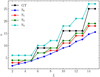Fig. 1. Number of rays per octant, n = N/8, as a function of the order L of the quadrature. We note that, in the case of the S0 quadratures, n is generally not an integer. See the text for more details.

The main result shown in this figure is that the S₀ quadrature type, that is, the most general one that lacks any rotational or reflection symmetry, is more efficient than the quadratures found in Paper I (the S₁ type, see the blue line in Fig. 1). For L = 15, the S₁ quadrature needs about 16% more rays than the S₀ quadrature. We also applied the node elimination algorithm to the S₁ quadratures studied in Paper I (shown with a red line in Fig. 1) and we verified that the number of rays is identical as previously reported.

The S₂ quadratures are typically slightly worse in terms of number of rays than S₁ but the difference is quite small up to L = 15. The GT quadratures also belong to the S₂ family as a special case, but their analytical accuracy is significantly worse (see the green and black lines in Fig. 1).

The worst performance is found in the case of the S₃ quadratures (see the cyan line in Fig. 1). These quadratures have the highest level of symmetries and, therefore, they are easy to find numerically. However, given that their accuracy is even worse than the GT quadratures, which can be generated without any numerical effort, there is no practical benefit in using the S₃ quadratures, apart from the fact that the rays are more equally distributed over the unit sphere than in the case of the GT quadratures.

Figure 2 shows an example of three near optimal quadratures S₀, S₂, and S₃ of order L = 13. We note that, in the case of the S₀ quadrature (left panel), the rays in the first octant do not determine the rays in the other octants due to the lack of symmetries. The S₀ quadratures need fewer rays than the other quadratures to achieve a given accuracy. This is because all the rays over the unit sphere are independent and can be more efficiently distributed. For the other quadratures, the independent (generating) rays are limited to a small region and used redundantly.

Fig. 2. Examples of near optimal angular quadratures of order L = 13. Left panel: S0 quadrature with a total of 100 independent rays. Central panel: S2 quadrature with 8 independent rays and 120 rays in total. Right panel: S3 quadrature with 5 independent rays and 168 rays in total. We note that although only one octant is shown, the independent rays in the left panel are distributed over the whole sphere. The blue points indicate the generating nodes while the red points are on their orbits.

3.2. Tests in a 3D non-LTE simulation

In the derivation of the near optimal quadratures, we restrict the expansion of the Stokes parameters up to a certain order L of the SH. In fact, this always leads to approximate quadratures. Indeed, the smoother the angular variation of the radiation field, the more accurate the expansion of Eq. (1).

In Paper I, we presented an example of how the amplitudes of the expansion coefficients (I_j)_ℓ decrease with the order ℓ (see Eq. (16) and Fig. 2 therein). This can be used for obtaining an empirical determination of the maximum order L required in a particular type of model.

There is no a priori guarantee that two different types of quadratures with the same order L will lead to the same accuracy in 3D non-LTE calculations in which Eq. (1) provides merely an approximation of the radiation field. Some of the quadratures may provide better accuracy than others when integrating the radiation field with a non-negligible contribution of the ℓ >  L modes. This is a model-dependent problem and we study it in this section using non-LTE radiative transfer in a 3D model of the solar atmosphere.

In order to check the actual accuracy on the $J_Q^K$ tensors using the new angular quadratures, we solved the non-LTE radiative transfer problem for polarised light in a 3D model resulting from a MHD simulation (Gudiksen et al. 2011; Carlsson et al. 2016), using the radiative transfer code PORTA² (Štěpán & Trujillo Bueno 2013). Due to the significant computing demands of 3D non-LTE radiative transfer and the high number of different quadratures to test, we decided to reduce the horizontal spatial resolution of the model grid by a factor of 6 at the expense of having more abrupt spatial variations on the physical parameters. The horizontal spatial resolution is approximately 240 km after the degradation. The vertical resolution remains the same as in the original model. The spectral line considered here is the strong resonance transition of neutral calcium at 422.7 nm. This transition can be modelled using a two-level model atom, with total angular momenta J_ℓ = 0 and J_u = 1 for the lower and upper levels, respectively. As for the reference values of the $J_Q^K$ tensors, we consider the fully converged solution using a very fine GT quadrature with 400 rays per octant, namely 20 per inclination and 20 per azimuth (20 × 20).

Our test of the quadratures consists in computing the self-consistent non-LTE solution using some new quadratures and constructing the histogram of errors with respect to the reference solution. To perform this test we use the values of the relevant quantities (i.e. $J_Q^K$) at the atmospheric height where the optical depth at line centre is unity for the line of sight along the vertical axis of the model.

Firstly, we test the S₁ quadratures presented in Paper I. We use the quadrature sets L = 9, 13 and 15 with 8, 14, and 18 rays per octant, respectively. We compare such solutions with the 3 × 3, 4 × 4, and 5 × 5 GT quadratures. Such sets solve the system of Eq. (3) up to the same order L as the S₁ quadratures (see Fig. 1). In Fig. 3 we show the relative errors of the radiation field tensors, $J_Q^K$, for the different quadratures. We see that both types of quadratures show the same accuracy, while the S₁ quadratures contain fewer rays. At L = 9, both quadratures have a significant relative error for the tensor components K ≠ 0, however, the mean intensity ($J_0^0$) is quite accurately calculated. The big relative errors in the tensors with K >  0 indicate how sensitive the polarisation calculations are to the accuracy of the angular quadrature.

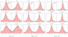Fig. 3. Histograms showing the relative errors in the percentage of the radiation field tensors, $(J_Q^K-{\left[J_Q^K\right]}_{\text{ref}})/{\left[J_Q^K\right]}_{\text{ref}}$, with respect to the reference solution, ${\left[J_Q^K\right]}_{\text{ref}}$, at the corrugated surface where the optical depth at the line centre is unity along the disc centre line of sight. The different panels show: (a) GT 3 × 3 and S1 with 8 rays per octant, (b) GT 4 × 4 and S1 with 14 rays per octant, and (c) GT 5 × 5 and S1 with 18 rays per octant.

Once we have checked that the S₁ quadratures work well, we can compare them with the other near optimal quadratures S₀ and S₂. We considered the same orders as before, L = 9, 13, and 15. In Fig. 4, we show the relative differences for each tensor component. We see that the quadratures with the same order provide similar accuracy. Therefore, those with fewer number of rays are superior even in the 3D calculations. For the L = 9 case (see the left panels of Fig. 4), we see that the S₂ quadrature provides a somewhat better accuracy than the others, while the difference disappears in the higher orders. We speculate that this may be an accidental relic of the particular 3D model we used. This model is not large enough to be representative of an average atmosphere in a statistical sense. This can be seen in the difference between the histograms of Re[$J_2^2$] and Im[$J_2^2$], which should look practically identical provided the model is sufficiently representative of the average atmosphere.

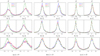Fig. 4. Histograms showing the relative errors in percentage of the radiation field tensors, $(J_Q^K-{\left[J_Q^K\right]}_{\text{ref}})/{\left[J_Q^K\right]}_{\text{ref}}$, at the height where the optical depth at the line centre is unity along the disc centre line of sight. The different panels show the histograms for different truncation orders of the spherical harmonics expansion for the S0, S1, and S2 quadratures with the following number of rays in total, respectively: (a) 62, 64 and 72 rays, (b) 100, 112 and 120 rays, and (c) 124, 144 and 152 rays in total.

4. Discussion and conclusions

In this paper, we have derived new sets of near optimal angular quadratures for the numerical solution of 3D radiative transfer problems of polarised radiation. We have generalised the methods formulated in Paper I and the new quadratures we have found are superior to those published previously.

The new quadrature rules derived in this work have different transformation symmetries than the previous ones. Imposing the new symmetries, we can simplify considerably the numerical problem because the system has fewer unknowns and fewer equations to be solved. In particular, the new groups of symmetry we have considered are defined in Eqs. (7) and (8). In addition, we have investigated angular quadratures without any particular symmetry.

Such new angular quadratures were calculated using our implementation of the node elimination algorithm developed by Xiao & Gimbutas (2010). Our experience shows that this algorithm is a powerful tool since, in most cases, the solution converges from any reasonable initial guess. However, since it is a depth-first search algorithm, the time complexity of each iteration for a new set of rays is 𝒪(N_g). This implies that finding a solution for a very high L can take a significant computing time, especially for angular quadratures without any kind of symmetries. However, we note that our algorithms were entirely implemented in Python and much faster solvers could probably be developed in compiled languages.

The only assumption applied in the derivation of our angular quadratures is that the angular variation of the radiation field has a certain level of smoothness. Such an assumption comes into play in Eq. (1), where the finite value of L determines the maximum order of spherical harmonics up to which the radiation field can be expanded and for which the calculation of the radiation field tensors will be exact. A similar limitation is inevitable for any finite quadrature. However, it is possible to adapt our methods to find less general quadratures that would be more accurate in particular astrophysical applications.

The S₀ quadratures have proven to be the best option for RT with polarised radiation. Given the required accuracy, they outperform other quadratures in terms of number of rays (16% less rays than S₁ and 36% less than the GT quadrature for L = 15). This is true both in the analytical calculations, as demonstrated in Fig. 1, as well as in realistic 3D simulations, as shown in Fig. 4. The tables with the different sets of the S₀ quadratures, both for the polarised case and for just the specific intensity, are available at the CDS.

It is not surprising that quadratures with a very high degree of symmetry cannot compete with the most general setup. However, quadrature sets with some kind of symmetry, such as that of the S₁ set, can be significantly easier to find numerically even for much larger values of L than we have considered in this work. However, robust techniques, such as the node elimination algorithm, need to be employed instead of a naive brute-force solution.

In our calculations, we forced the rays to avoid any octant edges, the poles, and the equator. Our argument for this is purely technical given that in some of the RT codes, such as PORTA, it is convenient to avoid such types of rays. This restriction does not affect the S₀ quadratures because they are not defined with respect to the octant boundaries, but it may, at least in principle, create unnecessary constraints for the other sets.

Acknowledgments

J.J.B. acknowledges financial support from the Spanish Ministry of Economy and Competitiveness (MINECO) under the 2015 Severo Ochoa Programme MINECO SEV–2015–0548. J.Š. acknowledges the financial support of grant 19-20632S of the Czech Grant Foundation (GAČR) and from project RVO:67985815 of the Astronomical Institute of the Czech Academy of Sciences. J.T.B. acknowledges the funding received from the European Research Council (ERC) under the European Union’s Horizon 2020 research and innovation programme (ERC Advanced Grant agreement No. 742265), as well as through the projects PGC2018-095832-B-I00 and PGC2018-102108-B-I00 of the Spanish Ministry of Science, Innovation and Universities. J.Š. and J.T.B. acknowledge the support from the Swiss National Science Foundation through the Sinergia grant CRSII5-180238. The authors thankfully acknowledge the technical expertise and assistance provided by the Spanish Supercomputing Network (Red Española de Supercomputación), as well as the computer resources used: the MareNostrum supercomputer in Barcelona and LaPalma Supercomputer.

References

All Figures

	Fig. 1. Number of rays per octant, n = N/8, as a function of the order L of the quadrature. We note that, in the case of the S0 quadratures, n is generally not an integer. See the text for more details.
In the text

Fig. 2. Examples of near optimal angular quadratures of order L = 13. Left panel: S0 quadrature with a total of 100 independent rays. Central panel: S2 quadrature with 8 independent rays and 120 rays in total. Right panel: S3 quadrature with 5 independent rays and 168 rays in total. We note that although only one octant is shown, the independent rays in the left panel are distributed over the whole sphere. The blue points indicate the generating nodes while the red points are on their orbits.

In the text

Fig. 3. Histograms showing the relative errors in the percentage of the radiation field tensors, $(J_Q^K-{\left[J_Q^K\right]}_{\text{ref}})/{\left[J_Q^K\right]}_{\text{ref}}$, with respect to the reference solution, ${\left[J_Q^K\right]}_{\text{ref}}$, at the corrugated surface where the optical depth at the line centre is unity along the disc centre line of sight. The different panels show: (a) GT 3 × 3 and S1 with 8 rays per octant, (b) GT 4 × 4 and S1 with 14 rays per octant, and (c) GT 5 × 5 and S1 with 18 rays per octant.

In the text

Fig. 4. Histograms showing the relative errors in percentage of the radiation field tensors, $(J_Q^K-{\left[J_Q^K\right]}_{\text{ref}})/{\left[J_Q^K\right]}_{\text{ref}}$, at the height where the optical depth at the line centre is unity along the disc centre line of sight. The different panels show the histograms for different truncation orders of the spherical harmonics expansion for the S0, S1, and S2 quadratures with the following number of rays in total, respectively: (a) 62, 64 and 72 rays, (b) 100, 112 and 120 rays, and (c) 124, 144 and 152 rays in total.

In the text

References

- Ahrens, C., & Beylkin, G. 2009, Proc. R. Soc. A Math. Phys. Eng. Sci., 465, 3103 [Google Scholar]
- Carlsson, M., Hansteen, V. H., Gudiksen, B. V., Leenaarts, J., & De Pontieu, B. 2016, A&A, 585, A4 [NASA ADS] [CrossRef] [EDP Sciences] [Google Scholar]
- Gudiksen, B. V., Carlsson, M., Hansteen, V. H., et al. 2011, A&A, 531, A154 [NASA ADS] [CrossRef] [EDP Sciences] [Google Scholar]
- Landi Degl’Innocenti, E., & Landolfi, M. 2004, Polarization in Spectral Lines (Astrophysics and Space Science Library), 307 [Google Scholar]
- Štěpán, J., & Trujillo Bueno, J. 2013, A&A, 557, A143 [NASA ADS] [CrossRef] [EDP Sciences] [Google Scholar]
- Štěpán, J., Jaume Bestard, J., & Trujillo Bueno, J. 2020, A&A, 636, A24 [CrossRef] [EDP Sciences] [Google Scholar]
- Xiao, H., & Gimbutas, Z. 2010, Comput. Math. Appl., 59, 663 [CrossRef] [Google Scholar]