| Issue |
A&A
Volume 645, January 2021
|
|
|---|---|---|
| Article Number | A83 | |
| Number of page(s) | 9 | |
| Section | The Sun and the Heliosphere | |
| DOI | https://doi.org/10.1051/0004-6361/202039120 | |
| Published online | 14 January 2021 | |
Evaluation of a potential field source surface model with elliptical source surfaces via ballistic back mapping of in situ spacecraft data
University of Kiel, Institute for Experimental and Applied Physics, Leibnizstr. 11, 24118 Kiel, Germany
e-mail: This email address is being protected from spambots. You need JavaScript enabled to view it.
Received:
7
August
2020
Accepted:
2
November
2020
Abstract
Context. The potential field source surface (PFSS) model is an important tool that helps link the solar coronal magnetic field to the solar wind. Due to its simplicity, it allows for predictions to be computed rapidly and requires little input data, though at the cost of reduced accuracy compared to more complex models. So far, PFSS models have almost exclusively been computed for a spherical outer boundary or “source surface”. Changing this to an elliptical source surface holds promise to increase its prediction accuracy without the necessity of incorporating complex computations or additional model assumptions.
Aims. The main goal of this work is to evaluate the merit of adding another parameter, namely the ellipticity of the source surface, to the PFSS model. In addition, the applicability of the PFSS model during different periods of the solar activity cycle as well as the impact of the source surface radius are analyzed.
Methods. To evaluate the model, in situ spacecraft data are mapped back to the source surface via a ballistic approach. The in situ magnetic field polarity is compared to the magnetic field polarity predicted by the model at the source surface. This method is based on the assumption that better performing models provide better agreements between the prediction and the measured magnetic field polarity. We employ data from the Advanced Composition Explorer and the twin Solar Terrestrial Relations Observatory (STEREO) for this analysis.
Results. We show that the PFSS model performs slightly better with oblate elliptical source surfaces elongated along the solar equatorial plane, although the best found ellipticity varies for different spacecraft and periods. In addition, it is demonstrated that the performance of the presented analysis degrades during the active times of the solar activity cycle.
Key words: Sun: magnetic fields
© ESO 2021
1. Introduction
The magnetic field of the inner solar corona plays a vital role in the acceleration processes of the solar wind. Due to the sparse availability of in situ measurements, there is a widespread need for computational models to predict the coronal magnetic field based on remote sensing observations. One of the earliest models is the potential field source surface (PFSS) model (Schatten et al. 1969; Altschuler & Newkirk 1969), which requires only synoptic line-of-sight magnetograms of the solar photosphere.
To obtain a configuration of the coronal magnetic field, the PFSS model assumes that there are no electric currents between the photosphere and a second virtual surface, the eponymous source surface, which is located a few solar radii higher. In addition, it is assumed that the magnetic field configuration is stationary for the duration of an entire Carrington rotation. The model, which employs two boundary conditions on the photosphere and the source surface, can produce a magnetic field configuration using a straightforward mathematical framework. The lower boundary condition is realized by deriving values for the magnetic potential from synoptic magnetograms. The upper boundary condition is implemented by keeping the magnetic potential constant throughout the solution process, thereby restricting the magnetic field direction to be perpendicular to the source surface. We refer to Mackay & Yeates (2012) for a more in-depth explanation of the exact model paradigm and variations of the PFSS models.
Although there are more complex models that offer the computation of a larger set of physical phenomena, namely full magnetohydrodynamic (MHD) models, the PFSS model is still widely used as a first-order approximation of the solar magnetic field for further analyses or where only large-scale magnetic field configurations are of interest. Other models that improve the PFSS model without adding the complexity of full MHD models exist, such as the current sheet source surface (CSSS) model (Zhao & Hoeksema 1995).
Several authors have suggested that deviating from the strict constraint of the source surface being spherical could increase the accuracy of solar magnetic field predictions by the PFSS model (Schulz et al. 1978; Schulz 1997; Levine et al. 1982; Riley et al. 2006). Kruse et al. (2020) altered the well-established spherical PFSS model to employ oblate and prolate elliptical source surfaces, removing the constraint that the magnetic field be radial at the same height at all latitudes. Spherical source surfaces assume an isotropic coronal magnetic orientation, whereas observations (see, e.g., McComas et al. 1998a) show a clear deviation of physical phenomena from this symmetry. An elliptical source surface can account for latitudinal differences of physical phenomena by allowing for different source surface heights and corresponding magnetic orientations.
The idea presented by Kruse et al. (2020) is to stretch out the spherical surface either above the solar equator or above the poles to obtain an oblate or prolate ellipsoidal source surface, respectively. Figure 1 shows cuts through various source surfaces of different ellipticities to be used with the new solver. The solar rotation axis is aligned vertically, and the lower boundary (i.e., the photosphere) is the same as in the spherical model.
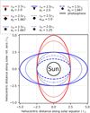 |
Fig. 1. Cuts through several source surfaces used in our PFSS models. Prolate source surfaces (red shapes) resemble zeppelin-shapes aligned with the solar rotation axis elongated along one axis, whereas oblate source surfaces (blue shapes) resemble thick disks elongated along two axes. The classical spherical source surface is drawn with a dotted black line. Various symbols introduced in the legend are used in Figs. 3–5, where they are shown at the corresponding positions. |
Evaluating the validity of predictions made by the PFSS model is complicated because the solar magnetic configuration can neither be simply reproduced in a clean laboratory environment nor measured remotely with high accuracy. Instead, the scientific community is forced to work with sparsely available in situ magnetic field spacecraft data (Hoeksema et al. 1983; Hoeksema 1984; Neugebauer et al. 1998; Badman et al. 2020), derive the magnetic field configuration from optical observations of the inner solar corona, such as white-light images or extreme ultraviolet (EUV) maps (Altschuler & Newkirk 1969; Smith & Schatten 1970; Levine et al. 1982; Lee et al. 2011), or compare the results of the PFSS model with the results of more intricate MHD models (Riley et al. 2006; Schulz et al. 1978; Schulz 1997).
The assumptions of the PFSS model are more often violated during the solar activity maximum than during the minimum. Therefore, the model is expected to perform worse during the solar maximum. To quantify this effect and illustrate the shortcomings of the model during the solar activity maximum, we performed the analysis in different periods of the solar activity cycle.
In the following, we present a method for comparing the magnetic field polarity predictions made by the PFSS model at the source surface to the in situ measurements of the near-Earth interplanetary magnetic field (IMF) taken by three spacecraft, namely the twin Solar Terrestrial Relations Observatory (STEREO-A and STEREO-B) and the Advanced Composition Explorer (ACE). The connection between these two locations is accomplished via ballistic back mapping along the Parker spirals from the spacecraft down to the source surface. We evaluate the two parameters, source surface height and ellipticity, using this back mapping polarity measure.
2. Methods
In the absence of laboratory setups, there are two major possibilities for evaluating the quality of solar magnetic field models. The first is an analysis of remote sensing data, such as white-light images of the solar corona or EUV images of the photosphere (see, e.g., Zhao et al. 2017; Huang et al. 2019). The second option is a comparison of in situ measurements of the IMF to values predicted by the model (see, e.g., Bale et al. 2019; Badman et al. 2020). The problem with the former method, due to the absence of high-resolution remote sensing magnetic field measurements above the lower corona, is the necessity of additional assumptions to derive the actual magnetic field configuration from these images. White-light images can be easily computed from predictions of MHD models because these models also compute the particle number density in the computational domain (see, e.g., Mikić et al. 2018). To the contrary, the PFSS model only calculates the magnetic field. Producing an image for comparison to remote sensing images without the knowledge of the particle density is, in our experience, not reliable. Nevertheless, it is feasible to draw magnetic field lines over coronagraph images and compare the overall orientation of magnetic to optical features, though projection effects impede conclusive or quantitative statements when comparing model parameters that might only slightly alter the magnetic field configuration.
Another method of evaluating the merits of solar magnetic field models via remote sensing instrumentation is to analyze the brightness of the synoptic EUV maps of the photosphere (see, e.g., Lee et al. 2011). Open magnetic field lines (i.e., those that reach the source surface) are typically associated with darker regions in the EUV spectrum. Therefore, a better model is expected to, on average, map the footpoints of open magnetic field lines to darker spots in the EUV spectrum. While this is a worthwhile analysis, it poses several problems: Depending on the wavelength of the analyzed EUV map, light emission originates in a thin sheet above the photosphere rather than in the photosphere itself. This will lead to some projection effects, similar to but not as strong as with white-light imaging. The average brightness of the EUV maps is dependant on the solar activity cycle; therefore, some form of normalization needs to be applied. Additionally, because the analysis concentrates on the lower boundary of the PFSS model, the upper boundary, where the model differs the most from the spherical model, is not examined.
Due to these shortcomings, we chose to first employ the second method of analyzing in situ measurements for evaluating the PFSS model and will leave the EUV method for another investigation. The problem with in situ measurements is the gap between available measurements (which are mostly obtained near 1 AU) and the regime of interest, which, in the case of the PFSS model, only spans a few solar radii above the photosphere. Therefore, it is necessary to map the in situ measurements of the solar wind parcels to the regime where they originated to have a reliable proxy for the remote magnetic field.
Section 2.1 describes the elliptical PFSS model that is evaluated here. In Sect. 2.2, we discuss the general procedure of tracking in situ measured solar wind packages to the source surface of the PFSS model and comparing predicted and observed magnetic field polarity. To better focus on the most interesting solar wind observations, we describe how to partition the measured solar wind data into meaningful categories according to the four-class Xu−Borovsky-scheme discussed in Sect. 2.3. We perform the analysis for three different periods during solar activity cycles 23 and 24. One period investigates the declining solar activity cycle nearing solar activity minimum, one analyzes the solar activity minimum, and one performs the same method during solar activity maximum. The analyzed periods and utilized instrumentation are discussed in Sect. 2.4.
2.1. Elliptical PFSS model
To incorporate elliptical source surfaces into the paradigm of the PFSS model, we need a numerical grid that is spherical at the photosphere and incrementally morphs into the desired elliptical shape with increasing height. The parameter of the source surface height is substituted for the minimum source surface height  , and a second parameter (i.e., the ellipticity) is added, which determines the maximum deviation from the spherical shape at the highest position in the numerical grid (i.e., at the source surface). In the oblate case, the minimum source surface height is found above the poles, while in the prolate case, it is found above the solar equator (see Fig. 1).
The ellipticity parameter defines how the maximum source surface height compares to the minimum source surface height  . Because our model employs a case-differentiation for the oblate and prolate ellipsoidal source surfaces, we denote the ellipticity parameter in the oblate case with eo and in the prolate case with ep. An ellipticity of eo = 2.0 in the oblate case means that the equatorial source surface height is twice the polar source surface height, and, in the prolate case, ep = 2.0 denotes a source surface that is twice as high at the poles compared to the equator. In Fig. 1, the two red shapes are prolate ellipsoids with a minimum source surface height of
  , where R⊙ is the solar photospheric radius. A growing prolate ellipticity parameter stretches the grid in the polar direction while the (minimum) equatorial source surface height remains unaltered. Similarly, in the oblate case, the grid is stretched in the equatorial direction with increasing oblate ellipticity while the minimum source surface height above the poles remains the same. Therefore, to keep a constant source surface height above the equator with increasing oblate ellipticity, the minimum source surface height (above the poles) has to be reduced, which is visualized by the blue shapes in Fig. 1.
Our numerical solver utilizes finite differences and an Euler stepping algorithm to obtain a solution to Laplace’s equation at all grid points. The grid we use for all analyses presented here has 35 × 87 × 175 grid points. The grid points are equidistant in the zonal direction, equidistant in sine-latitude in the meridional direction, and have a geometrically increasing spacing in the radial direction. The Laplace operator was derived for general curvilinear coordinates and adjusted for our special case. More information on the technical details of the solver and differences in predicted polarity and heliospheric current sheet locations between the spherical and elliptical solvers is available in Kruse et al. (2020).
2.2. Back mapping polarity measure
Because the solar wind flows radially away from the Sun, it carries with it the frozen-in magnetic field, which thus forms an Archimedean spiral. Assuming that the plasma parcel being investigated flows at a constant solar wind speed from the source surface to the observer, the footpoint of the magnetic field line (the Parker spiral) on the source surface is easily calculated. Let  be the rigid rotational speed of the Sun and vp the solar wind bulk flow speed measured at the spacecraft. The zonal ballistic footpoint position Φfp of the spacecraft position Φsc on an arbitrary heliocentric height r can be obtained via the equation
 (1)
(1)
where rsc is the heliocentric distance of the spacecraft.
Having obtained a position on the source surface, we can then extract the magnetic polarity predicted at that position by our various PFSS implementations and compare it to the magnetic polarity measured aboard the spacecraft down from which the plasma package was traced. Figure 2 shows a schematic of the measurement configuration. If the polarities are the same, we note a correctly predicted sample. If they differ, we note a false prediction. The overall fraction of correctly predicted samples serves as our quality metric, where higher numbers denote better predictions.
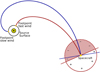 |
Fig. 2. Ecliptic view of the experimental setup (not to scale). Theoretical paths of fast (red) and slow (blue) solar wind packages traced from the spacecraft down to the source surface constitute two coordinate frames. The magnetic polarity is defined by the projection of the magnetic field vector onto the Parker spiral in the respective frame. Two hemispheres are separated by a plane perpendicular to each Parker spiral (colored accordingly). A vector has a positive sign if it lies within the anti-sunward hemisphere (pointing outward, solid half-circle) and has a negative sign if it lies within the sunward hemisphere (pointing inward, dashed half-circle). The depicted hemispheres illustrate the situation in the fast solar wind frame. The slow wind frame has two hemispheres that are defined analogously. |
The back mapping polarity measure is noticeably simple, as even just guessing the polarity of a large number of samples would yield a 50% correct prediction rate. A sufficient implementation needs to be significantly better than this 50% threshold. Furthermore, the polarity alone does not give insight into the correctness of the magnetic configuration below the source surface. Nevertheless, this metric allows us to compare different implementations and periods relative to one another: An implementation that does not even get the polarity right is not assumed to perform better in absolute terms compared to one that does.
As a variability measure of this metric, we employed a form of cross-validation using the following method. Each analysis spans several Carrington rotations. Let N denote the number of full Carrington rotations observed. Instead of computing the fraction of correctly mapped samples for the entire period, we computed N sets of fractions where, for each set, another Carrington rotation is excluded from the analysis. Let pm, i denote the fraction of correctly mapped samples where Carrington rotation i (i ∈ {0,…,N−1}) is excluded. The final value of this metric is the average over all data sets,  . The standard deviation of this data set,
  , is used as an error or variability measure of the analysis.
2.3. Selection of data samples
Not all solar wind observations give the same insight into the validity of the underlying model of the solar magnetic field. We expect the most interesting results for regions where the polarity of the large-scale magnetic field changes, that is to say, we try to mostly analyze solar wind packages that originated near current sheet crossings.
We partitioned the whole data set according to the Xu & Borovsky (2015) solar wind categorization scheme into four categories. The first is coronal-hole plasma, historically also known as the fast solar wind, which originates above open magnetic structures mostly near high latitudes. The second type is called streamer belt plasma, which is believed to originate near the edges of coronal holes. The third and most interesting type for our analysis is sector reversal plasma, which is likely emitted around helmet streamers where the polarity of the coronal magnetic field changes its polarity. The last type of solar wind is called the ejecta type and is associated with dynamic and short-lived processes like coronal mass ejections. Because the PFSS model is a static model, we do not expect it to be able to predict any dynamic processes; therefore, we omit this wind type from further analysis. We also omit coronal-hole plasma because we do not expect many magnetic polarity changes.
The Xu & Borovsky (2015) scheme requires four types of in situ measurements; they are the proton temperature Tp, bulk flow velocity vp, proton number density np, and magnetic field strength B. Although the hyperplanes that separate the solar wind types in this four-dimensional space have been derived for the instruments aboard the ACE spacecraft, we also employed this scheme to the twin STEREO spacecraft, which are roughly at the same heliocentric height as ACE and therefore are expected to measure similar characteristics of the solar wind.
Here we mostly concentrate on sector reversal wind and streamer belt wind. This way, we can take a closer look at solar wind streams that feature specific behaviors where this metric might yield the most interesting results, namely, the locations of the current sheet crossings. Furthermore, we excluded plasma packages that were identified to be part of interplanetary coronal mass ejections (ICME) according to the lists of Cane & Richardson (2003), Richardson & Cane (2010), and Jian et al. (2018) as these plasma streams have different characteristics than the previously stated radial expansion of the unperturbed solar wind. They are also inconsistent with the basic assumptions of the PFSS model that demand a static coronal magnetic field configuration.
The Xu−Borovsky scheme is not a perfect partition of the solar wind. Due to the strict boundaries in the four-dimensional parameter space, and without context-sensitive measures, there will always be falsely identified plasma packages. In addition, the solar magnetic field exhibits so-called kinks (see, e.g., Berger et al. 2011), where the overall large-scale polarity is disturbed by short periods of opposite polarity. While a correction of these factors might be beneficial for the analysis, there is the risk of introducing new errors into the data sets by employing an untested correction scheme. We, therefore, chose to accept these minor flaws in the evaluation presented here. We estimate the difference in prediction accuracy due to short-lived polarity reversals in Sect. 3.3.
2.4. Evaluated periods and instrumentation
An analysis of large data sets would be desirable to increase the validity of the obtained results. Unfortunately, high-resolution space-bound photospheric magnetogram data have only been available for less than three decades. It would be preferable to analyze the same stages of the solar activity cycle in different individual cycles, but we only have the three decades’ worth of data. Therefore, we chose ten Carrington rotations from a single cycle for each of the three stages of interest. In period 1, we investigate the declining solar activity phase of solar cycle 23 during Carrington rotations 2041 to 2055 (in 2006), excluding rotations 2044, 2046, 2047, 2050, and 2053. Period 2, which analyzes the minimum between solar activity cycles 23 and 24, consists of Carrington rotations 2066 to 2075 (in 2008), and period 3, which examines the solar activity maximum of cycle 24, is comprised of Carrington rotations 2133 to 2142 (in 2013). Because we want to examine EUV maps in future studies, we excluded some rotations from the declining period that had missing data in either the utilized magnetograms or the corresponding EUV maps. The magnetograms for the minimum and maximum periods 2 and 3 had better coverage, but we also have fewer Carrington rotations to choose from; we therefore decided not to exclude any rotations from these periods.
The utilized photospheric magnetograms for the PFSS computation were obtained from the Michelson Doppler Imager (MDI; Scherrer 1995) aboard the Solar and Heliospheric Observatory (SOHO) spacecraft for periods 1 and 2 and from the Helioseismic and Magnetic Imager (HMI; Scherrer et al. 2012) aboard the Solar Dynamics Observatory (SDO), the successor spacecraft to SOHO. Unfortunately, MDI data are not available for the third period. Synoptic magnetograms of complete Carrington rotations were used for the analysis.
For the back mapping analysis, we chose data from ACE (Stone et al. 1998) and the twin STEREO (Kaiser et al. 2008) mission. All three spacecraft operate in the ecliptic plane near Earth’s orbit. Solar wind speeds at ACE were measured by the Solar Wind Electron, Proton, and Alpha Monitor (SWEPAM; McComas et al. 1998b) as well as by the Solar Wind Ion Composition Spectrometer (SWICS; Gloeckler et al. 1998). We utilized a merged 12 min SWICS/SWEPAM data set. For the STEREO spacecraft, we used a one-minute data set for solar wind speeds that were measured by the Plasma and Suprathermal Ion Composition (PLASTIC) instruments (Galvin et al. 2008). In situ measurements of the magnetic field were carried out on the STEREO spacecraft by the In situ Measurements of Particles and CME Transients (IMPACT) suite (Luhmann et al. 2008; Acuña et al. 2008) and by the Magnetic Fields Experiment (MAG) onboard ACE (Smith et al. 1998).
For the back mapping polarity measure, data from the two instruments aboard each spacecraft are required to have the same sampling rates. This means we had to resample the four-minute data set from MAG aboard ACE to match the 12 min cadence of the merged SWICS/SWEPAM data set. All data sets of instruments aboard the STEREO spacecraft have a cadence of one minute, so resampling was not necessary for the STEREO spacecraft. We also created data sets of the same cadence (12 min) to analyze the influence of the sampling rate but found no noticeable difference in the results; we therefore chose to utilize the higher sampling rates of the STEREO instrumentation.
3. Results: Magnetic field polarity prediction accuracy
To employ the PFSS model, assumptions about the coronal plasma have to be simplified. This largely refers to the premises that there are no electric currents between the photosphere and the source surface and that there are stable conditions during an entire Carrington rotation. We know that these assumptions are never completely true, but the question remains of whether they are accurate enough during the solar cycle to warrant the usage of the PFSS model for the prediction of the magnetic configuration.
Our findings for the spherical PFSS model with the widely accepted best source surface radius of 2.5 R⊙ are summarized in Sect. 3.1. We then investigate the impact of the ellipticity of the source surface on the accuracy of the prediction, which we present in Sect. 3.2.
3.1. Accuracy of prediction throughout the solar cycle
Table 1 shows the fraction of samples that have the same polarity measured in situ aboard the spacecraft and at the source surface as predicted by the PFSS implementations. We used our grid implementation of the spherical PFSS model with a radial lower boundary condition (Altschuler & Newkirk 1969) and with a source surface radius of 2.5 R⊙.
Back mapping polarity measure for the spherical source surface at 2.5 R⊙.
Solar wind that has been classified as ejecta probably originated in non-current-free regions, for which the basic assumptions of the PFSS model are not valid; therefore, the back mapping will likely not point to the correct source region. Coronal hole wind originates far outside of regions with expected magnetic polarity changes; hence a high fraction of correctly matched polarities is not surprising. Streamer belt and sector reversal wind constitute the most interesting data sets as they originate close to the current sheet where most polarity changes take place. As can be seen in Table 1, polarity prediction during solar maximum is much less accurate compared to the solar minimum. This is not surprising because the basic assumptions that the region below the source surface is current-free and stationary during an entire Carrington rotation are violated more often during solar maximum. Especially for the sector reversal wind, where most current sheet crossings take place, the prediction accuracy drops to almost 50%, illustrating the shortcoming of the PFSS model during the active part of the solar activity cycle.
3.2. Dependence of prediction accuracy on source surface ellipticity
To determine the impact of a nonspherical surface on the coronal magnetic field, we repeated the back mapping analysis while varying the ellipticity and minimum source surface height parameters. In the following, we focus only on the more interesting solar wind types, namely sector reversal and streamer belt. Figure 3 depicts the results for period 1 (CR2041−CR2055) of the declining solar activity cycle. For period 2 (CR2066−CR2075) during solar minimum, the STEREO twin spacecraft mission was operational; therefore, in addition to back mapping from ACE, we have computed the back mapping prediction accuracy from STEREO-A and from STEREO-B in Fig. 4. The active Sun was analyzed during period 3 (CR2133−CR2142), and the results can be found in Fig. 5.
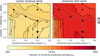 |
Fig. 3. Back mapping polarity measure for streamer belt and sector reversal wind. Ballistic back mapping was performed from ACE to the source surface during period 1 (CR2041−CR2055, 2006, declining solar activity). The colored pixels give the value at their center positions (black dots) in 2% increments. A contour plot bi-linearly interpolating between these values has been drawn on top. Lines marking model parameters of constant equatorial source surface height have been inserted for rss, equ = 2.5 R⊙ (solid gray line), for rss, equ = 2.0 R⊙ (dotted gray line), and for rss, equ = 3.0 R⊙ (dashed gray line). The black symbols mark the parameters for the example source surfaces from Fig. 1. |
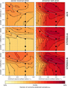 |
Fig. 4. Back mapping polarity measure for period 2 (CR2066−CR2075, 2008, solar activity minimum) for spacecraft ACE, STEREO-A, and STEREO-B. The format is the same as in Fig. 3. |
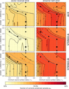 |
Fig. 5. Back mapping polarity measure period 3 (CR2133−CR2142, 2013, solar activity maximum). The format is the same as in Figs. 3 and 4. |
To better illustrate the meaning of the two parameters of our implementation, we depict cuts through various source surfaces in Fig. 1. As can be seen from this figure, increasing the ellipticity in the prolate case does not alter the equatorial source surface height, while in the oblate case, the equatorial height increases with increasing ellipticity. To keep the equatorial height constant with increasing ellipticity, the minimum source surface height  has to be decreased. As all measurements from ACE, STEREO-A, and STEREO-B are made near the ecliptic, the equatorial source surface height plays a major role in our back mapping polarity measure. Moving within the figures to higher prolate ellipticities along the negative y-axis has a different effect than moving along the positive y-axis to higher oblate ellipticities. Because the analysis presented here only samples regions near the solar equator, major changes in other regions are not reflected. The most notable changes in the magnetic field configuration in the prolate models are present at higher latitudes, which are not sampled. This has to be kept in mind when interpreting Figs. 3–5. It also explains why there are fewer structures depicting the prolate source surfaces in the lower half of these figures. The magnetic field near the solar equator changes more notably with increasing oblate ellipticity than it does with increasing prolate ellipticity.
As can be seen from Figs. 3–5, back mapping polarity prediction performs noticeably worse for the active sun period 3 compared to the minimum period 2. This is to be expected as the assumption of a quasi-stationary environment breaks down when the Sun’s activity cycle approaches its maximum. Furthermore, when comparing ACE back mapping in the declining and minimum periods 1 and 2, the PFSS model performs slightly better in the minimum period 2, with more pronounced peaks in the parameter space. The differences between the declining and maximum periods 1 and 3 are not as prominent as between the minimum and maximum periods 2 and 3. During the declining period 1 and the activity maximum period 3, the plateaus of best parameters are broader compared to the activity minimum period 2.
During the minimum period 2 (Fig. 4), the best agreement between the three spacecraft can be found in the streamer belt wind. The best prediction ratio of more than 80% for all spacecraft can be found at a minimum source surface radius of slightly above  and an oblate source surface ellipticity of about eo = 1.5, which amounts to an equatorial source surface radius of roughly rss, equ = 3.0 R⊙. For the sector reversal wind, the data are less clear. Firstly, the overall prediction ratio is substantially worse compared to the streamer belt wind, which is to be expected as this set contains the interesting current sheet crossings. Secondly, the position of the maximum varies strongly between the spacecraft. Thirdly, there is no clear single peak; the region of best prediction is broad. The figures suggest the best prediction ratio for slightly lower source surfaces with higher oblate ellipticities compared to the streamer belt data sets.
There are clear differences between the three spacecraft in the minimum and maximum periods 2 and 3. One major distinction is, of course, the instrumentation used for measuring in situ solar wind speed and magnetic configuration. In this regard, STEREO-A and STEREO-B results are at least mutually comparable as both are equipped with near-identical instruments. However, the Xu−Borovsky solar wind categorization scheme was developed using ACE data, so the classification process for the two STEREO spacecraft might be prone to errors, which affects the overall prediction ratios. STEREO-A is slightly closer to the sun than ACE, which is slightly closer than STEREO-B. Therefore, the difference in the position of the maximum in these plots might be attributable to the variation of the respective heliocentric distances, although they are still small compared to 1 AU.
3.3. Influence of short-lived polarity reversals
The heliospheric magnetic field exhibits short-lived polarity reversals that are not part of the large-scale magnetic field. The PFSS model is not able to resolve these so-called kinks of the magnetic field because they are local structures that are the result of wave-particle-interaction and turbulent processes. Thus, it would be desirable to filter out these kinks. A simple technique is to compute a running average of the magnetic field, thereby eliminating most of the polarity reversals that have a shorter duration than the window width of the averaging method. The problem with this method is that polarity reversals with a solar origin, which are relevant for the analysis, will be affected as well. Therefore, we chose not to filter the data set and to accept lower overall prediction ratios. The study presented here relies less on the absolute values of the prediction ratio than on relative changes and the position of the maximum in the two-dimensional parameter space. To estimate the impact of short-lived polarity reversals, we repeated the analysis for the minimum period 2 and spacecraft ACE with a running average and a window width of 15 samples, that is, a width of 180 minutes. This leads to a higher maximum in the parameter space of 2% for the sector reversal wind type, 6% for coronal-hole wind, and 8% for streamer belt samples. However, it is important to note that for the streamer belt samples and the sector reversal wind type, this increase in the prediction accuracy is in part caused by removing some of the relevant but particularly difficult polarity reversal with solar origin from the data set. More complex filtering techniques, for example considering the direction of the electron heat flux (Owens et al. 2017), could be applied to increase the prediction ratio without affecting polarity reversals with a solar origin; however, this is beyond the scope of this work.
4. Conclusions
We have presented a PFSS model with elliptic source surfaces and the back mapping polarity measure to evaluate it, as well as the data selection procedure to partition in situ solar wind spacecraft data into meaningful categories according to the Xu & Borovsky (2015) scheme. Not surprisingly, our results show that the predictability of the solar magnetic field polarity is better during solar minimum compared to solar maximum. While the fractions of correctly predicted samples pm in the sector reversal wind are still slightly above the 50% threshold of pure guesswork, the usefulness of the PFSS model during solar maximum for prediction of the coronal magnetic configuration is superficial at best. Our findings show that, during solar activity maximum, the most accurate, albeit still unsatisfactory, predictions can be made for source surfaces with an equatorial height of 2.5 R⊙. The ellipticity parameter does not have a strong impact on the back mapping polarity measure during this period.
During the period of the solar activity minimum, our results suggest that the model performs better for slightly oblate elliptical source surfaces compared to the classical spherical model. The resulting equatorial source surface height is about rss, equ = 3 R⊙. This result is supported by data from all three spacecraft employed for this analysis in both sector reversal and streamer belt wind, although the exact parameters differ slightly. However, because our analysis was necessarily limited to the equatorial region, a definitive best set of parameters for all regions cannot yet be extracted from these findings. Our findings are also in stark contrast to those of Schulz et al. (1978), Schulz (1997), and Levine et al. (1982), who found that source surfaces with a greater height above the poles compared to the equator match the observations best. We would also like to mention that the visible peaks of the best parameter set stand only slightly higher in the parameter space than the surroundings with respect to the error of the back mapping polarity measure (see Table 1 and Figs. 3–5).
For a better prediction of the optimal parameters, a larger data set needs to be analyzed. Back mapping analysis from spacecraft outside of the ecliptic could give valuable insight into the magnetic configuration of elliptical PFSS models at higher latitudes. However, the Xu & Borovsky (2015) scheme was developed for instruments near 1 AU in the ecliptic plane, and therefore another partitioning scheme of solar wind streams is required for the analysis (e.g., Zhao et al. 2017). Ulysses and Solar Orbiter are the only two spacecraft outside the ecliptic that feature the instrumentation needed for this sort of analysis, with Solar Orbiter being the better option due to its lower perihelion distance. The higher heliocentric distance of Ulysses introduces more errors when ballistically mapping to the source surface due to the longer travel time of the plasma packages. Optimal parameters probably differ for different Carrington rotations as well.
We used a comparison of the in situ measured magnetic field polarity with that calculated at the source surface as the test metric and showed that the predictive power of an elliptic PFSS is not much better than that of a spherical PFSS model. We suspect that the elliptical model may hold a more substantial advantage over the spherical model for prediction accuracy in the corona below the source surface. Tracing the solar wind packages downward from the source surface to the photosphere is possible because the charged particles need to follow the magnetic field lines. Analyzing these photospheric footpoints in EUV images might provide another tool for evaluating the merit of nonspherical source surfaces, complementing the analysis presented here.
Acknowledgments
This work utilizes data from the Michelson Doppler Imager aboard SOHO. SOHO is a project of international cooperation between ESA and NASA. Magnetograms from HMI aboard SDO are courtesy of NASA/SDO and the AIA, EVE, and HMI science teams. Data from NASA’s STEREO and ACE missions were used for this work. We thank the STEREO IMPACT and PLASTIC teams as well as the ACE SWICS, SWEPAM and MAG teams for making the data available to the scientific community.
References
- Acuña, M. H., Curtis, D., Scheifele, J. L., et al. 2008, Space Sci. Rev., 136, 203 [NASA ADS] [CrossRef] [Google Scholar]
- Altschuler, M. D., & Newkirk, G. 1969, Sol. Phys., 9, 131 [Google Scholar]
- Badman, S. T., Bale, S. D., Martínez Oliveros, J. C., et al. 2020, ApJS, 246, 23 [CrossRef] [Google Scholar]
- Bale, S. D., Badman, S. T., Bonnell, J. W., et al. 2019, Nature, 576, 237 [NASA ADS] [CrossRef] [Google Scholar]
- Berger, L., Wimmer-Schweingruber, R. F., & Gloeckler, G. 2011, Phys. Rev. Lett., 106, 151103 [NASA ADS] [CrossRef] [Google Scholar]
- Cane, H. V., & Richardson, I. G. 2003, J. Geophys. Res.: Space Phys., 108, 1156 [Google Scholar]
- Galvin, A. B., Kistler, L. M., Popecki, M. A., et al. 2008, Space Sci. Rev., 136, 437 [NASA ADS] [CrossRef] [Google Scholar]
- Gloeckler, G., Cain, J., Ipavich, F. M., et al. 1998, Space Sci. Rev., 86, 497 [NASA ADS] [CrossRef] [Google Scholar]
- Hoeksema, J. T. 1984, PhD Thesis, Stanford University, USA [Google Scholar]
- Hoeksema, J. T., Wilcox, J. M., & Scherrer, P. H. 1983, J. Geophys. Res., 88, 9910 [NASA ADS] [CrossRef] [Google Scholar]
- Huang, G.-H., Lin, C.-H., & Lee, L.-C. 2019, ApJ, 874, 45 [CrossRef] [Google Scholar]
- Jian, L. K., Russell, C. T., Luhmann, J. G., & Galvin, A. B. 2018, ApJ, 855, 114 [NASA ADS] [CrossRef] [Google Scholar]
- Kaiser, M. L., Kucera, T. A., Davila, J. M., et al. 2008, Space Sci. Rev., 136, 5 [NASA ADS] [CrossRef] [Google Scholar]
- Kruse, M., Heidrich-Meisner, V., Wimmer-Schweingruber, R. F., & Hauptmann, M. 2020, A&A, 638, A109 [CrossRef] [EDP Sciences] [Google Scholar]
- Lee, C. O., Luhmann, J. G., Hoeksema, J. T., et al. 2011, Sol. Phys., 269, 367 [Google Scholar]
- Levine, R. H., Schulz, M., & Frazier, E. N. 1982, Sol. Phys., 77, 363 [CrossRef] [Google Scholar]
- Luhmann, J. G., Curtis, D. W., Schroeder, P., et al. 2008, Space Sci. Rev., 136, 117 [NASA ADS] [CrossRef] [Google Scholar]
- Mackay, D. H., & Yeates, A. R. 2012, Liv. Rev. Sol. Phys., 9, 6 [Google Scholar]
- McComas, D. J., Bame, S. J., Barraclough, B. L., et al. 1998a, Geophys. Res. Lett., 25, 1 [NASA ADS] [CrossRef] [Google Scholar]
- McComas, D. J., Bame, S. J., Barker, P., et al. 1998b, Space Sci. Rev., 86, 563 [NASA ADS] [CrossRef] [Google Scholar]
- Mikić, Z., Downs, C., Linker, J. A., et al. 2018, Nat. Astron., 2, 913 [Google Scholar]
- Neugebauer, M., Forsyth, R. J., Galvin, A. B., et al. 1998, J. Geophys. Res., 103, 14587 [NASA ADS] [CrossRef] [Google Scholar]
- Owens, M. J., Lockwood, M., Riley, P., & Linker, J. 2017, J. Geophys. Res.: Space Phys., 122, 10,980 [NASA ADS] [CrossRef] [Google Scholar]
- Richardson, I. G., & Cane, H. V. 2010, Sol. Phys., 264, 189 [NASA ADS] [CrossRef] [Google Scholar]
- Riley, P., Linker, J. A., Mikić, Z., et al. 2006, ApJ, 653, 1510 [Google Scholar]
- Schatten, K. H., Wilcox, J. M., & Ness, N. F. 1969, Sol. Phys., 6, 442 [Google Scholar]
- Scherrer, P. 1995, https://doi.org/10.5270/esa-9kpubs2 [Google Scholar]
- Scherrer, P. H., Schou, J., Bush, R. I., et al. 2012, Sol. Phys., 275, 207 [Google Scholar]
- Schulz, M. 1997, Annal. Geophys., 15, 1379 [CrossRef] [Google Scholar]
- Schulz, M., Frazier, E. N., & Boucher, D. J. 1978, Sol. Phys., 60, 83 [CrossRef] [Google Scholar]
- Smith, S. M., & Schatten, K. H. 1970, Nature, 226, 1130 [CrossRef] [Google Scholar]
- Smith, C. W., L’Heureux, J., Ness, N. F., et al. 1998, Space Sci. Rev., 86, 613 [NASA ADS] [CrossRef] [Google Scholar]
- Stone, E. C., Frandsen, A. M., Mewaldt, R. A., et al. 1998, Space Sci. Rev., 86, 1 [Google Scholar]
- Xu, F., & Borovsky, J. E. 2015, J. Geophys. Res.: Space Phys., 120, 70 [NASA ADS] [CrossRef] [Google Scholar]
- Zhao, X., & Hoeksema, J. T. 1995, J. Geophys. Res., 100, 19 [NASA ADS] [CrossRef] [Google Scholar]
- Zhao, L., Landi, E., Lepri, S. T., et al. 2017, ApJ, 846, 135 [Google Scholar]
All Tables
All Figures
|
Fig. 1. Cuts through several source surfaces used in our PFSS models. Prolate source surfaces (red shapes) resemble zeppelin-shapes aligned with the solar rotation axis elongated along one axis, whereas oblate source surfaces (blue shapes) resemble thick disks elongated along two axes. The classical spherical source surface is drawn with a dotted black line. Various symbols introduced in the legend are used in Figs. 3–5, where they are shown at the corresponding positions. |
| In the text | |
|
Fig. 2. Ecliptic view of the experimental setup (not to scale). Theoretical paths of fast (red) and slow (blue) solar wind packages traced from the spacecraft down to the source surface constitute two coordinate frames. The magnetic polarity is defined by the projection of the magnetic field vector onto the Parker spiral in the respective frame. Two hemispheres are separated by a plane perpendicular to each Parker spiral (colored accordingly). A vector has a positive sign if it lies within the anti-sunward hemisphere (pointing outward, solid half-circle) and has a negative sign if it lies within the sunward hemisphere (pointing inward, dashed half-circle). The depicted hemispheres illustrate the situation in the fast solar wind frame. The slow wind frame has two hemispheres that are defined analogously. |
| In the text | |
|
Fig. 3. Back mapping polarity measure for streamer belt and sector reversal wind. Ballistic back mapping was performed from ACE to the source surface during period 1 (CR2041−CR2055, 2006, declining solar activity). The colored pixels give the value at their center positions (black dots) in 2% increments. A contour plot bi-linearly interpolating between these values has been drawn on top. Lines marking model parameters of constant equatorial source surface height have been inserted for rss, equ = 2.5 R⊙ (solid gray line), for rss, equ = 2.0 R⊙ (dotted gray line), and for rss, equ = 3.0 R⊙ (dashed gray line). The black symbols mark the parameters for the example source surfaces from Fig. 1. |
| In the text | |
|
Fig. 4. Back mapping polarity measure for period 2 (CR2066−CR2075, 2008, solar activity minimum) for spacecraft ACE, STEREO-A, and STEREO-B. The format is the same as in Fig. 3. |
| In the text | |
|
Fig. 5. Back mapping polarity measure period 3 (CR2133−CR2142, 2013, solar activity maximum). The format is the same as in Figs. 3 and 4. |
| In the text | |
Current usage metrics show cumulative count of Article Views (full-text article views including HTML views, PDF and ePub downloads, according to the available data) and Abstracts Views on Vision4Press platform.
Data correspond to usage on the plateform after 2015. The current usage metrics is available 48-96 hours after online publication and is updated daily on week days.
Initial download of the metrics may take a while.