| Issue |
A&A
Volume 645, January 2021
|
|
|---|---|---|
| Article Number | A32 | |
| Number of page(s) | 14 | |
| Section | Astronomical instrumentation | |
| DOI | https://doi.org/10.1051/0004-6361/202038853 | |
| Published online | 24 December 2020 | |
Bolometric night sky temperature and subcooling of telescope structures
1
European Southern Observatory (ESO), Karl-Schwarzschild-Str. 2, 85748 Garching, Germany
e-mail: This email address is being protected from spambots. You need JavaScript enabled to view it.
2
Institut für Astro- und Teilchenphysik, Leopold–Franzens Universität Innsbruck, Technikerstr. 25, 6020 Innsbruck, Austria
3
Instituto de Astronomía, Universidad Católica del Norte, Av. Angamos 0610, Antofagasta, Chile
4
Institut für Physik, Universität Augsburg, Universitätsstraße 1, Augsburg 86159, Germany
5
Deutsches Fernerkundungsdatenzentrum, Deutsches Zentrum für Luft- und Raumfahrt (DLR), Münchener Straße 20, Weßling-Oberpfaffenhofen 82234, Germany
Received:
6
July
2020
Accepted:
2
October
2020
Abstract
Context. The term sky temperature is used in the literature to refer to different phenomena in different contexts which often leads to confusion. In this work, we study Tsky, the effective bolometric sky temperature at which a hemispherical black body would radiate the same power onto a flat horizontal structure on the ground as the night sky, integrated over the entire thermal wavelength range of 1–100 μm. We then analyze the thermal physics of radiative cooling with special focus on telescopes and discuss mitigation strategies.
Aims. The quantity Tsky is useful to quantify the subcooling in telescopes which can deteriorate the image quality by introducing an optical path difference (OPD) and induce thermal stress and mechanical deflections on structures.
Methods. We employ the Cerro Paranal Sky Model of the European Southern Observatory to derive a simple formula of Tsky as a function of atmospheric parameters. The structural subcooling and the induced OPD are then expressed as a function of surface emissivity, sky view factor, local air speed, and structure dimensions.
Results. At Cerro Paranal (2600m) and Cerro Armazones (3060m) in the Atacama desert, Tsky towards the zenith mostly lies 25–50 Kelvin below the ambient temperature near the ground, depending to a great extent on the precipitable water vapor column in the atmosphere. The temperature difference can decrease by several Kelvin for higher zenith distances. The subcooling OPD scales linearly to quadratically with the telescope diameter and is inversely proportional to the local air speed near the telescope structure.
Key words: telescopes / instrumentation: miscellaneous / atmospheric effects / site testing / radiative transfer / convection
© ESO 2020
1. Introduction
Any structure on the ground that is exposed to the night sky experiences a radiation imbalance and therefore typically cools below the ambient air temperature (see Zhao et al. 2019 for an overview). Sky subcooling is strongest at sites with low water vapor column, hence under conditions commonly present at telescope sites (high and dry). As a consequence, the air surrounding a steel truss for example is cooled, causing a wake of cool air. Light rays passing the cooled air experience an optical path difference which induces a transient wavefront error in a telescope (Wilson 2013). This situation is most severe at small wind speeds and thus became known as the “low-wind effect”, and has recently been studied (Sauvage et al. 2015; Milli et al. 2018). A secondary detrimental consequence of subcooling is structural deflection due to thermal contraction, inducing mechanical stress and optical misalignment. Quantifying the effective sky temperature is therefore required when designing advanced ground-based telescopes and analyzing their image quality.
Previous studies (Berdahl & Fromberg 1982; Gliah et al. 2011; Sun et al. 2017; Li et al. 2017, 2018) used wide-angle integrating detectors subtending nearly the whole sky. Moreover, these detectors are tested and calibrated at sites with lower altitudes and higher humidity. To derive the effects of the sky temperature on a telescope structure and the optical elements such as the main mirror, a detailed understanding of sky irradiance as a function of the direction on the sky is required as well. To our knowledge, such a study has not yet been published.
In Sect. 2, we discuss the night-sky emissivity and define the effective bolometric sky temperature Tsky. Section 3 then sets up a thermal balance model of a structure on the ground exposed to sky radiation and forced convection. Furthermore, we discuss the effects of heat conduction and thermal inertia. Finally, we conclude in Sect. 4.
2. Sky radiance and sky temperature
The spectrum of the radiance Lsky for a given area on the sky irradiating a surface strongly depends on wavelength λ, zenith distance θ, and weather conditions. Its total bolometric radiance EBOL, defined as the integral of the radiance spectrum over all wavelengths, is dominated by those fractions of the wavelength domain where the atmosphere is completely opaque. In these regions, the mean free path of the light is often a few hundred meters only; in optically very thick lines it may even be only a few meters. Thus the main emission is strongly bound to the local temperature near the ground. Those regions where the atmosphere is nearly transparent do not significantly contribute to the integrated radiance. We use here the common definition of a sky temperature Tsky as the equivalent temperature of a black-body radiation curve of the same bolometric radiance EBOL (see Li et al. 2017, 2018, and references therein),
 (1)
(1)
where the unit is W m−2 sr−1, with the Stefan–Boltzmann constant σ = 5.670367 × 10⁻⁸ W m−2 K−4.
2.1. General trend and climatology of the sky temperature
With our European Southern Observatory (ESO) Sky Model1 (Noll et al. 2012; Jones et al. 2013) we are able to calculate detailed spectral dependencies and integrate them to derive the bolometric flux and the sky temperature Tsky. Although this sophisticated model contains a wide variety of components of illumination such as scattered moonlight, zodiacal light, scattered starlight, and atomic and molecular emission lines in the upper atmosphere (airglow), the vast majority of the bolometric flux originates from about 4 to 7 μm and longwards of 13.5 μm and is dominated by the emission of the lower atmosphere. Our model uses a spectral model of the Earth’s lower atmosphere in local thermal equilibrium calculated by means of the Line-By-Line Radiative Transfer Model (LBLRTM; Clough et al. 2005). This code is used with the spectral line parameter database aer, which is based on HITRAN (Rothman et al. 2009). Averaged atmospheric profiles for Cerro Paranal describing the chemical composition as a function of height (a combination of the ESO ambient Meteo Monitor, a standard atmosphere for low latitudes2, and the 3D Global Data Assimilation System (GDAS) model) are also used as input. The GDAS model is provided by the National Oceanic and Atmospheric Administration (NOAA)3 and contains time-dependent profiles of temperature, pressure, and humidity. For the sky model, bimonthly averages over several years were built yielding reliable forecasts for typical conditions at Cerro Paranal. For the transmission and thermal emission of the atmosphere, the current model can be adapted to any site if appropriate GDAS profiles are used. Clear cloudless weather conditions are required with the LBLRTM standard setup.
We show the dependency of the thermal sky radiance as a function of precipitable water vapor (PWV) in Fig. 1. This quantity is equal to the integrated column density across the whole atmosphere, including all layers contributing to the opaqueness, and is given in units of equivalent thickness in millimeters of liquid water. The opaque fraction of the spectral energy distribution resembles a black body radiation curve. While the transparency in the window around λ = 10 μm is only marginally affected by the H2O molecular bands, it varies strongly in the region from 15 to 28 μm (astronomical Q-band) with the water vapor content. Therefore, the weather-dependent variations and uncertainties mainly originate from this wavelength band. There are marginal transparency windows beyond these wavelengths (astronomical mid-infrared Z-band with 28 < λ < 40 μm). As shown by Yoshii et al. (2010), this assumption still holds at sites of even higher altitude than Mauna Kea (e.g., as planned for the 6.5 m Tokyo Atacama Telescope project at 5640 m). Therefore, an approximation with a black body curve is normally sufficient. The ozone absorption in the center of the N-band does not follow the trend of the other opaque regions because of the high altitude of the absorbing molecules.
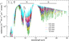 |
Fig. 1. Sky radiance Lsky(λ) for Cerro Paranal at different PWV conditions typical for observations in the direction of zenith. The astronomical observation bands and the main ozone absorption are marked. For further details on species that are not important for us here (e.g., CO2, N2O and CH4) see Fig. 1 and Table 1 in Smette et al. (2015). |
The sky radiance (expressed as sky temperature as defined above) therefore depends significantly on the PWV. This circumstance was already found by Berdahl & Fromberg (1982), but these latter authors characterized the measured radiation as a function of the relative humidity near the ground, specifically the dew point temperature TDP calculated from the humidity. Although radiation from low altitudes prevails, the variation is dominated by semi-transparent regions in the Q-band. Here we see radiation from higher layers having different temperatures and a water vapor content which is not necessarily linked to the relative humidity measured near the ground.
We find a phenomenological fit function of the sky temperature with the water vapor content for dry conditions (Fig. 2) which is precisely passing the points with deviations of less than 0.1 K. In more humid conditions (PWV > 15 mm) the relation still fits rather well, but has some larger uncertainties, on the order of 2 K. Although the fit is based on model data for the southern winter months June and July, it is also valid for the other months of the year. The small differences in the bimonthly mean profiles of pressure and temperature, as well as the relative vertical distribution of water vapor at Cerro Paranal, appear to have a negligible effect on the integrated radiance spectrum.
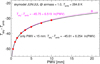 |
Fig. 2. Correlation of the sky temperature Tsky and PWV at zenith Only the range of conditions with PWV < 15 mm relevant for typical astronomical observations is used for the final fit function. |
Moreover, previous studies (Berdahl & Fromberg 1982; Gliah et al. 2011; Sun et al. 2017; Li et al. 2017, 2018) used wide-angle integrating detectors subtending almost the whole sky. However, in order to calculate a radiation model for a structure, the irradiation of this structure as a function of its exposed direction to the sky has to be taken into account (see also Sect. 3.2). This effect is not as important for a structure such as a whole building or a solar cell, as studied by Berdahl & Fromberg (1982) or Li et al. (2017) for example. These latter authors therefore needed only integrated values for the entire sky. However, structures of a telescope inside a dome are exposed in a more complex way to different fractions of the sky. Thus, the exact spatial impacts are essential. When tilting the telescope to higher zenith distances, the radiation is increasingly dominated by low heights. Therefore, we derived the correlation of the irradiance with zenith distance for a wide variety of parameters (Fig. 3). A comparison of the summer and winter models shows a very good match of the data points. There are only marginal differences for θ = 60° and 70°. Therefore, again, a general season-independent fit can be derived. We find that this correlation does not depend on humidity after accounting for the zenith dependency mentioned above, and a direct empirical fit function with both parameters for good weather conditions (PWV < 15 mmH2O and no clouds) is found:
 (2)
(2)
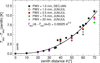 |
Fig. 3. Correlation of the sky temperature Tsky and zenith distance at a constant level of PWV. |
where Tamb is the ambient temperature near the ground in Kelvin, PWV is in mmH2O, and the zenith distance θ is measured in degrees.
2.2. Individual solutions and local estimators
Our software molecfit (Smette et al. 2015; Kausch et al. 2015) was originally designed to correct astronomical spectra for telluric absorption. However, it can also be used to simulate individual thermal emission spectra for a certain date and time at a site. The code automatically derives the GDAS profile of that very day and time from the servers.
In order to test extreme weather conditions that are not well represented by the sky model, we calculated emission spectra for the warmest and the coldest nights with respect to local midnight at Cerro Paranal in July 2018 (Fig. 4). The reference temperatures were measured 30 meters above ground at the ambient monitoring station. They agree well with the temperatures that are derived from a fit of a black body to only those regions in the spectrum where the atmosphere is very opaque. For comparison, we also considered the warmest and coldest nights in 2018 at the high-altitude site at Mauna Kea observatory in Hawaii, as measured at the weather monitor of the Canada-France-Hawaii Telescope (CFHT). This observatory site has significantly lower air temperatures due to its high altitude of 4200m (Fig. 5). Therefore, the relative humidity at this altitude tends to be lower. However, the latter and the dew point temperature calculated from it (Buck 1981) are only loosely correlated with the integrated water vapor column, that is, the scatter is large (Otárola et al. 2010). Therefore, we have to use PWV (indicating the impact of the most important and highly variable trace gas H2O) to optimally parameterize the atmospheric radiation (Otárola et al. 2010; Lakićević et al. 2016).
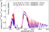 |
Fig. 4. Sky radiance at zenith on the coldest and the warmest days at Cerro Paranal (2600m) in July 2018. The fit of a black body is based on the marked points only, defining an upper boundary. |
While we were able to take the PWV measured from the Low Humidity And Temperature PROfiler (L-HATPRO) microwave radiometer at Cerro Paranal (Kerber et al. 2012, see Sect. 2.3.1) for Fig. 4, the PWV values for Hawaii are only based on the (less accurate) GDAS profiles for the given nights. The PWV values and the resulting Tsky for the integrated sky spectrum and using Eq. (2) are provided in Table 1. The fit formula causes deviations in Tsky between −3.6 and +4.8 K for these extreme conditions, which suggests that its general uncertainty is not larger than a few Kelvin.

In cases where a sky model is not available at a given site, we tested the possibility of estimating the values of Tsky from the transmission curve. For the most part, the latter depends on the site altitude and the PWV (which can be obtained by means of GDAS data but might also be derived by various multi-wavelength observations without use of a model), and can therefore be easily tabulated for any site. Multiplying this transmission curve with a black body spectrum only depending on the ambient temperature Tamb results in the desired estimator  after integration over all wavelengths (Eq. (1)). As indicated in Figs. 4 and 5, such an estimate can almost perfectly match the accurate radiative transfer model result and confirms the parameterization in Eq. (2). Only the ozone band from 9.6 to 10.1 μm is strongly overestimated because most of the ozone emission originates from a higher layer in the atmosphere with a lower temperature. This kind of emission might be different for very low-altitude sites near populated areas, but the latter is beyond our study. Therefore, the ozone-related wavelength range was excluded from the integration. Other regions with special molecular features do not seem to be dominant enough to significantly contribute to our result. The resulting estimated sky temperature
  in Table 1 does not deviate by more than 2.1 K from Tsky. For the more typical cases represented by the same parameters as used in Figs. 2 and 3,
  lies about 1.5 K above the value of the full model for PWV < 15mm (Fig. 6).
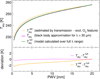 |
Fig. 6. Comparison of the sky temperature |


The ESO Sky Model yields radiation spectra only up to a wavelength of 30 μm. Above this region, pure black body emission is typically assumed in the standard online implementation (SkyCalc). The integration of that emission using Eq. (1) leads to Tsky used in the rest of the paper. This simplification leads to slight overestimation of the radiation for very dry conditions and high sites. However, a complete model by us using a custom patched version of the radiative transfer model ( ) shows that the correction to the formula given above is marginal for PWV > 1.0mm and even below. The discrepancies are of the order of only 0.2K (Fig. 6).
2.3. Ambient meteorological conditions at Cerro Paranal
2.3.1. Methods and data selection
At Cerro Paranal there are several astronomical site monitoring (ASM) systems installed which permanently record the atmospheric ambient conditions. We investigate data from a period of 4.5 years (2015-07-01T00:00:00 to 2019-12-31T23:59:59) based on the ESO Meteo Monitor, the L-HATPRO radiometer (Kerber et al. 2012), and the Differential Image Motion Monitor (DIMM). An overview of these data is given in Sarazin (2017). From the Meteo Monitor we extracted the wind direction, wind speed, and the ambient temperature Tamb measured at a height of 30 m (as in Sect. 2.2) as the telescope structure is more exposed to this part of the atmosphere than towards the ground (cf. Sect. 2.1).
The L-HATPRO radiometer database provides integrated PWV measurements at zenith (θ = 0°) and measurements of the infrared sky temperature TIR achieved by a specific infrared radiometer mounted at the L-HATPRO, which operates in the 9.6 to 11.5 μm band. As mentioned in Sect. 2.1, the Earth’s atmosphere is widely transparent in this wavelength range. Therefore, TIR measurements are very sensitive to (comparably warm) clouds at various heights. In particular, ice clouds (cirrus) can be detected, which is not possible with the microwave radiometer. The DIMM incorporates data on the seeing conditions and the sky transparency, the latter being measured by the relative root mean square (rms) of flux variations of reference stars along the line of sight during nighttime (normalized by the average flux).
We merged the data points of these three databases via their time stamps by finding the closest Meteo Monitor and DIMM neighbor to each individual radiometer measurement within Δt ≤ 300 s. By skipping those measurements with Δt > 300 s, we automatically restrict our merged data set to nighttime because the DIMM only provides data taken between dusk and dawn. We also omitted data points with invalid values and those with PWV ≤ 0.02 mm.
The data set should represent typical observing conditions at Cerro Paranal, that is, omitting poor weather conditions, which is important because the subcooling of the telescope structure (Sect. 3) is strongest in the best (= photometric) conditions. In addition, the ESO Sky Model does not cover cloudy conditions, and therefore Eq. (2) is not applicable. In order to exclude cloudy periods, we therefore apply a DIMM rms cut of 2% (which is consistent with the criterion for possible clouds of the online ASM tool at ESO). This cut reduces our sample by only about 10%; good photometric conditions prevail at Cerro Paranal. In total we select 276 958 data points.
2.3.2. Statistics on the meteorological data
Investigations of the overall yearly variability reveal a strong trend towards higher PWV values in the southern summer months with an annual median value of PWV ≈2.47 mm (10% percentile: 1.06 mm; 25% percentile: 1.56 mm; 75% percentile: 4.08 mm; 90% percentile: 6.39 mm). In addition, weather situations with winds coming from a 90° cone centered on the north are the most frequent ones (56% of the overall time), with a tendency towards higher wind speeds, higher PWV values, and more clouds. As our data selection criteria exclude most of the poor conditions, the sensitivity of our investigations with respect to the wind direction is minimized. Our empirical equation for Tsky (Eq. (2)) depends on PWV and the ambient temperature Tamb. We assume these quantities to be independent. Our data set can be used to test this assumption. Figure 7 does not show a clear correlation. This finding can be tested by the Pearson coefficient r, which indicates whether or not a data set shows a linear correlation (r = ±1 means perfect linear correlation, r = 0 no linear correlation). As the absolute value is small in our case (r = 0.16), we conclude that our parameterization of Tsky is justified. The distribution of Tsky given in Fig. 8 reveals a median value of Tsky = 246.2 K and a standard deviation of σ = 5.7 K for the selected clear observing conditions.
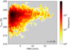 |
Fig. 7. Two-dimensional histogram of the ambient temperature Tamb as a function of PWV for clear observing conditions (see text for more details). The bin widths of the histogram are 0.1 mm in PWV and 0.5 K in Tamb. The resulting Pearson coefficient r is indicated (see text for more details). |
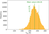 |
Fig. 8. Histogram of the calculated Tsky values; its mean value is 246.2 K, the standard deviation σ = 5.7 K. |
Figure 9 shows the infrared temperature TIR versus the sky temperature Tsky determined with Eq. (2), which was calculated by means of the Tamb values from the ESO Meteo Monitor at θ = 0°. As TIR has a relatively weak dependency on PWV but is strongly sensitive to even thin cirrus clouds (due to the small wavelength range used for the measurements), the infrared radiometer temperature is related to the sky temperature Tsky only in the case of photometric observing conditions and Tsky ≳ 240 K. It is therefore not a good estimator for the sky temperature and its effect on the subcooling of telescope structures. In contrast, Tsky derived by Eq. (2) provides a robust estimate for that purpose only based on measurements of the PWV, the ambient temperature, and the zenith distance θ.
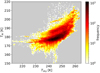 |
Fig. 9. Tsky vs. TIR at θ = 0° as two-dimensional histogram (bin width of 0.5 K) for clear observing conditions. |
2.4. Ambient meteorological conditions at Cerro Armazones
In Sect. 3, we compute numerical quantities using typical environmental conditions at Cerro Armazones, the site of the Extremely Large Telescope (ELT; 3 060 m; Koehler 2015; Otárola et al. 2019). The median nighttime air temperature is Tamb = 9.1° C = 282.25 K and the median air pressure equals p = 712 hPa. Measurements of PWV such as those taken with L-HATPRO at Cerro Paranal (Sect. 2.3.1) are not available for Cerro Armazones. Nevertheless, estimates by Otárola et al. (2010) and Lakićević et al. (2016) suggest that the median value for clear sky conditions at Cerro Paranal, namely 2.47 mm (Sect. 2.3.2), should be relatively similar. Possible systematic deviations of the order of half a millimeter are not critical for our purposes. Applying Eq. (2) for the selected PWV value, we obtain a difference between Tsky and Tamb of −39.9 K at zenith and −37.8 K at the typical observing zenith angle θ = 37°. With the ELT median Tamb, this results in Tsky of 242.4 K and 244.5 K, respectively.
Otárola et al. (2019) presented a cumulative wind statistic for Cerro Armazones. However, that study was focused on radio astronomy and thus included daytime data. Fortunately, the complete weather data are publicly available4 and we selected the nighttime wind data between 22 : 30 and 9 : 00 h UTC for the years 2006–2009. We find a nocturnal median wind speed at 7 meters above the ground of 7.0 m s−1, 33% of the time the wind speed is below 5.2 m s−1, 25% of the time below 4.3 m s−1 and 15% of the time below 3.0 m s−1.
From a related data set covering the years 2004–2008, we find that the median nocturnal temporal gradient of Tamb is equal to −0.34 K h−1 when the temperature is falling and +0.25 K h−1 when it is rising (which is relevant for significantly shorter time periods). The corresponding quartiles are −0.17 and −0.60 K h−1 (falling) versus +0.11 and +0.51 K h−1 (rising), respectively.
3. Thermal modeling of telescope structures
3.1. Radiative heat flux
In this section, we derive the steady-state temperature of a structure that radiatively cools against the night sky and is heated by forced convection of the ambient air. We consider a small surface of area A that has a spectral emissivity of ϵ(λ, γ), where γ is the angle between the surface normal n and the observing direction. The radiative heat flux from the sky that is absorbed by the surface can be written in spherical coordinates (centered at zenith) according to Lambert’s Cosine Law (Pedrotti & Pedrotti 1993) as
 (3)
(3)
 (4)
(4)
where Lsky is the spectral radiance from the sky (unit W m−2 sr−1m−1), γ = γ(θ, ϕ) and ϕ is the azimuth. Both θ and ϕ are measured in radians, in contrast to the previous section. If the surface is oriented horizontally (n points towards zenith), we find γ = θ and κ = cos(γ).
Conversely, to calculate the emitted flux  from the surface to the sky, one simply replaces Lsky(λ, θ, ϕ) in Eq. (3) by the black body spectral radiance
![Mathematical equation: $$ \begin{aligned} L_{\rm bb}(\lambda ,T_{\mathrm{surf}}) = \frac{2\, h_{\rm Pl} \, c^2}{\lambda ^5} \,\left[\exp \,\left(\frac{h_{\rm Pl}\, c}{\lambda \, k_B\, T_{\mathrm{surf}}}\right) - 1 \right]^{-1}, \end{aligned} $$](/articles/aa/full_html/2021/01/aa38853-20/aa38853-20-eq14.gif) (5)
(5)
where Tsurf is the surface temperature, hPl = 6.62618 × 10⁻³⁴ J s is Planck’s constant, kB = 1.38065 × 10⁻²³ J/K is Boltzmann’s constant, and c = 2.99792 × 10⁸ m s−1 is the speed of light in vacuum.
As shown in Figs. 4 and 5, the sky spectrum agrees with a black-body fit spectrum within several wavelength ranges (e.g., near 7 μm or near 15 μm). The temperature of this fit spectrum is close to the ambient air temperature at sites at higher altitudes. The radiation imbalance  is therefore dominated by the wavelength bands where Lsky(λ)−Lbb(λ) has a large magnitude, specifically in the astronomical N-band (7 – 13.5 μm) and the Q-band (17 – 25 μm). The area between the spectra and their respective fits in Figs. 4 and 5 provides a graphical representation of this relationship.
The wavelength- and angle-resolved emissivity ϵ(λ, γ) is often unknown. Working with an average emissivity  is possible, but it should be noted that its value is defined by the requirement to preserve the value
  of the wavelength integral in Eq. (3). Any emissivity weighted by the full black-body spectrum, as is sometimes provided by commercial measurement devices or listed in specification sheets, is not well suited to quantify subcooling. Instead, a better approximation is to only consider the emissivity around λ = 11 μm and, if available, around 18 μm.
3.2. Sky view factor
The relationship between spectral radiance and Tsky is (Zhao et al. 2019)
 (6)
(6)
in accordance with Eq. (1), where the angular brackets denote the geometrical averaging over the sky hemisphere.
Surfaces that are located inside buildings, such as a telescopes in a dome with open doors, can typically only see a solid angle Ω < 2π of the sky hemisphere. The sky view factor for a point q on the surface is defined by
 (7)
(7)
where the telescope transmission function 𝒯(θ, ϕ) is equal to 1 at directions θ, ϕ for which an unobstructed path from q to the sky exists and zero if the path is blocked by any warm black body. However, we also allow for partly obscured ray paths like propagation through a windscreen mesh or indirect ray paths to the sky through reflection on a mirror (often the primary mirror M1), or any partially reflective surface like a bare metal for which 0 < 𝒯 < 1. The normalization factor π−1 ensures that 0 ≤ Fsky ≤ 1.
The sky view factor for a horizontal surface inside a building with a circular aperture centered at n that is seen from q under the one-sided angle θa is equal to sin2(θa). This term assumes the value 1/2 at θa = 45°, although the solid angle of this aperture subtends only 29.3% of the hemisphere. If, on the other hand, the aperture is not centered at n, Fsky will be smaller. This reasoning shows that the orientation of surfaces inside a telescope dome is important, and not simply the distance from the dome slit. The difference is particularly large when comparing the sky view factors for the top side of the spider trusses (with rectangular cross section) or the secondary mirror housing (Fsky ≈ 0.8 – 1) with its side faces where n is perpendicular to the telescope axis. Under no circumstances can the side faces see more than half of the sky hemisphere (Fsky ≤ 1/2). Furthermore, the zenith angles θ at which the cosine weighting term κ is large are almost perpendicular to the telescope axis; more precisely, these rays may often point near the horizon (the side faces may even see part of the ground outside the telescope building). The average sky temperature is higher in these directions due to the θ 2.5 dependence; see Eq. (2).
When dealing with noncircular apertures to the sky (e.g., the open door slit of a telescope dome) as sketched in Fig. 10, it can be more convenient to work with Cartesian coordinates x, y, z. The effect of κ in Eq. (7) is simply to project the area of the sky hemisphere that can be seen from the point q onto the unit disk on the tangential surface (perpendicular to n). If we let ρ = (x, y, z) be a vector of unit length that points from q to the sky, and x, y, z are local coordinates, meaning that any vector (x, y, 0) lies on the tangential surface and n = (0, 0, 1), we can write
 (8)
(8)
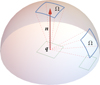 |
Fig. 10. Evaluation of sky view factors by projection. Red arrow: normal vector n above the point q on a surface. Blue quadrilaterals: two windows of solid angle Ω ≈ 0.16 sr through which the sky can be seen from q (i.e., 𝒯 = 1); the right window is tilted against n by γ = 60°. Green rectangles: projection of the windows onto the tangential plane with areas π Fsky ≈ Ω and Ω × cos(60° ) = Ω/2, respectively. |
In buildings, the sky windows often have much more complicated shapes than in Fig. 10. One can numerically evaluate Fsky in this case by describing the edges of the sky windows by a closed set of straight lines. The projected window then forms an (irregular) polygon on the unit disk whose area can be computed easily by the “shoelace formula” (Braden 1986). Dividing this area by π yields Fsky. Any window edges whose rays ρ would point below the tangential plane, that is, if γ ≥ 90° and thus κ = 0, generate projected points that lie on the unit circle in this scheme.
A collection of formulas to calculate Fsky in special geometries is found in Chapter 10 of Lienhard (2011).
If a structure is exposed to some part of the sky through a mirror, or in general through a series of reflective optics, Fsky is defined by the ray bundle emanating from q that ultimately reaches the sky, hence with 𝒯 > 0. In other words, the effective aperture is the image of the real aperture (say, the rim of the dome slit) as seen from q. One can compute Fsky by evaluating the angles γ of the ray segments between q and the first reflective surface. This method is correct even if the mirrors are powered (i.e., have nonzero curvature) by the principle of étendue conservation (Chaves 2017) and assuming that the sky is a Lambertian radiator (setting aside the dependence of Tsky on θ).
3.3. Thermal balance equation
With the help of Eqs. (3)–(7), we can write the radiative heat loss due to sky subcooling as Lienhard (2011)
 (9)
(9)
 (10)
(10)
where Tamb is the ambient air temperature inside the dome on the upwind side of the telescope structure and ΔTsurf quantifies the surface subcooling. The expression  denotes the average sky temperature with the same transmission 𝒯 as in Eqs. (7) and (8). As discussed in the previous section, this average geometrically depends on the patch of sky seen from q and the telescope pointing.
On the other hand, convection heats the surface at a rate of
 (11)
(11)
where h is the interface heat transfer coefficient (in units of W K−1 m−2). In thermal equilibrium and neglecting thermal conduction, we require that
 (12)
(12)
and therefore the heat fluxes are balanced. Our goal is to quantify the steady-state plate subcooling ΔTsurf < 0 that satisfies
 (13)
(13)
Expression (13) is a quartic equation with two real and two complex roots. One of the two real roots lies below −1300 K, and so there is only one meaningful solution. We calculated the latter in closed form, but the expression is rather complicated. Instead, we carry out a Taylor expansion to first order in ΔTsurf about ΔTsurf = δT. Solving for ΔTsurf, we obtain
 (14)
(14)
In the remainder of this paper, we choose δT = −3 K so that we cover the typical range of subcooling in telescopes of about −6 K ≤ ΔTsurf ≤ 0 with good accuracy.
Following Lienhard (2011), we define the radiation heat transfer coefficient
 (15)
(15)
and, rewriting Eq. (14), finally express ΔTsurf as
 (16)
(16)
 (17)
(17)
 (18)
(18)
where the number η quantifies the subcooling efficiency. We thus find that ΔTsurf scales linearly with η as long as η ≪ 1. We highlight that ΔTsurf ∝ 1/h in this unsaturated regime, which applies to most cases of interest in telescope subcooling. At ELT median conditions (Sect. 2.4), η is of the order of 0.1 and the subcooling is driven by the temperature offset ΔTD which equals −33.9 K for θ = 37°. In the opposite limit of η → ∞, we obtain ΔTsurf → ΔTsky := Tsky − Tamb. In practice, this extreme can probably only be reached on a black surface facing the sky inside a vacuum vessel with a window that transmits infrared radiation.
3.4. Convective heat transfer
The thermal coupling of a structure to the ambient air through forced convection gives rise to a boundary flow problem (Martinez 2020a). The convective heat transfer coefficient h depends on the air speed v near the surface (which is often much lower than the wind speed outside the dome), the air pressure p, and, to a great extent, on the shape of the structure. The structures closest to or even inside the telescope beam are usually steel trusses supporting the secondary and possibly the tertiary or quaternary mirrors. The simplest truss shape is cylindrical with diameter d. An approximate expression for hcyl, modeling the net heat exchange of airflow perpendicular to a cylinder, was derived by Churchill & Bernstein (1977). Their original formula is expressed in terms of the Reynolds, Nusselt, and Prandtl numbers (Martinez 2020b) and we checked that the values of these numbers for typical telescope structures are within the validity range of the formula. We do not reproduce the general formula here but instead simplify it to
 (19)
(19)
where c1 = 0.0179 W K−1 m−1, c2 = 1.5 × 10⁻⁴ for airflow at Tamb = 282 K, and s = π d is the cylinder circumference. We introduced the Reynolds number scaling quantity m, which equals 1.0 m W−1 if the incoming airflow is perfectly laminar and the cylinder has a smooth surface, and m ≈ 1.5 m W−1 for partly turbulent inflow. However, if a precision of more than about 20% in hcyl is demanded, one has to resort to computational fluid dynamics (CFD) simulations.
At v = 7.6 m s−1 and s = 0.6 π = 1.88 m, one reaches c2 β5/8 = 1. For much lower air speeds (more precisely, if β ≪ 1.3 × 10⁶), the scaling law hcyl ∝ (m p v/s)1/2 applies. We note that, although v = 7.6 m s−1 is close to the median wind speed on Cerro Armazones (cf. Sect. 2.4), the air speed inside the dome is often much lower. This holds in particular for structures below the M2 level, and therefore this regime is normally valid.
In the opposite limit of large β, for example for high air speed and/or large structures, hcyl ∝ β/s = m p v. The Reynolds number then becomes so large that the boundary layer is turbulent throughout, and thus the structure size is no longer relevant for hcyl. An example for this limit is subcooling of the outer dome cladding, where v approaches the free air wind speed and the interface length s can amount to tens of meters for streamlines that follow the dome surface.
Figure 11 shows a plot of hcyl for three different values of s representative of structures in the VLT and ELT telescopes and the ELT dome door (all for the ELT environmental conditions and m = 1.25 m W−1). Sundén et al. (2010) contains an overview of h for cylinders with noncircular cross sections.
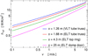 |
Fig. 11. Convective heat transfer coefficient hcyl vs. local air speed v for three different interface lengths s representative of structures in the VLT and ELT telescopes, plus the ELT dome door. |
Figure 12 shows a plot of ΔTsurf as a function of  according to Eq. (16), where the colors indicate four different local air speeds v. For these calculations and the remainder of this paper, we assume ELT median conditions as defined in Sect. 2.4 for the zenith angle θ = 37°. The colored fans in Fig. 12 are meant to give an impression of the influence of the interface length s : As s grows from s = 0.4 π m = 1.26 m to s = 4.3 m, hcyl diminishes and therefore η grows, and thus the subcooling intensifies. Consequently, subcooling becomes more severe as telescopes grow.
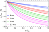 |
Fig. 12. Steady-state surface subcooling ΔTsurf as a function of |

Figure 13 is a two-dimensional plot of Tsurf(Fsky, v) for s = 4.3 m (ELT top ring truss circumference) and  , which is typical for dedicated low-emissivity paints; see Yarbrough (2010) for an overview of some respective commercial products. The tube structures of several large telescopes such as Gran Telescopio Canarias (GTC, La Palma), Keck I+II (Mauna Kea, Hawaii), and the two Gemini telescopes (Cerro Pachón, Chile, and Mauna Kea) are covered with LO/MIT5 paint by the company Solec (a silvery paint with small aluminum particles). On surfaces that scatter visible stray light, one may apply selective foil such as Acktar NanoBlack® 6 or Maxorb (Mason et al. 1982). These foils are black at visible wavelengths but highly reflective and thus low in emissivity (
 ) in the thermal infrared. Combining Eq. (19) with Eq. (16), we find a simplified fit function near
  and Fsky = 0.5 given by
 (20)
(20)
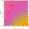 |
Fig. 13. Steady-state surface subcooling ΔTsurf as a function of Fsky and v for s = 4.3 m and |

where s is entered in meters and v is in meters per second, and again ΔTsky = Tsky − Tamb. We found the power laws of s and v using the rule b = x f′/f for a function f(x) = a xb with derivative f′, applied at s = 0.6 π m = 1.88 m and v = 1 m s−1.
3.5. Optical path difference
Temperature differences ΔT in an air volume cause the optical path length difference (OPD) of
 (21)
(21)
where q is a point in the air volume and l measures geometrical distance along the ray path. The refractive index of air n(λ, T, p) as a function of temperature T and pressure p is given by Edlen’s modified formula (Bönsch & Potulski 1998). Its derivative by T can be written in simplified form as
 (22)
(22)
where ρ = p/(Rair T) denotes the air density (Rair = 287.06 J kg−1 K−1 is the gas constant of dry air, yielding ρ = 0.879 kg m−3 at ELT median conditions) and the constant ρ0 = 4450 kg m−3 in the wavelength range 0.4 μm ≤ λ ≤ 3 μm.
At ELT median conditions, we obtain dn/dT = −9.828 × 10⁻¹² K−1 Pa−1 × p which is equal to −7.0 × 10⁻⁷ K−1. For the ray path from the top of the ELT secondary mirror (M2) crown level to M1, then back to M2 and finally to the prime focus of total length 36 m + 31 m + 13 m = 80 m, an air cooling as small as ΔT = 25 mK causes an accumulated OPD of 1.4 μm, equivalent to about 0.64 λ in K-band (2 – 2.4 μm). The thermal OPD is thus significant and may actually become the leading wavefront error contribution in 30-meter-class telescopes and greater.
In the following, we establish the link between the subcooling temperature offset ΔTsurf and the OPD. We rewrite the surface area in Eq. (11) as A = s L, where L is the length of a cylindrical truss that we assume to be oriented perpendicular to the local airflow vector v and perpendicular to the telescope optical axis, as would be the case for example for part of the top ring, as shown in Fig. 14.
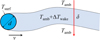 |
Fig. 14. Slice through a cylindrical truss of diameter d = s/π running perpendicular to v and to the telescope axis. Red arrow: ray of light traversing the cool wake of thickness δ and temperature difference ΔTwake. |
On the downwind side of the truss, a wake of cooled air is generated. We consider now a ray of light in a thin air slice perpendicular to v and assume for simplicity that the wake has a thickness along the ray of δ with constant temperature offset ΔTwake < 0. The total volume of cooled air flowing away from the truss per time Δt is then equal to V/Δt = δ L v and transports the heat flow
 (23)
(23)
where cp = 1005 J kg−1 K−1 is the specific heat capacity of air at constant pressure.
We can then derive the OPD imposed on the ray by the cooled air generated by a single truss of circumference s in a single ray pass by combining Eq. (23) with Eq. (11)
 (24)
(24)
In reality, the wake is of course not isothermal, but instead the temperature distribution depends on the aerodynamics and is nonstationary. However, the actual temperature distribution along the ray is immaterial for the problem at hand since the path integral in Eq. (21) is a conserved quantity equal to δ ΔTwake when averaged over time and along the truss length L. In the absence of this spatial and temporal averaging, transient vortexes can distribute air pockets of different temperature in the plane orthogonal to the rays (Martinez 2020b) generating a transient wavefront error; however, this aspect is beyond the scope of this work.
When hrad ≪ h (e.g., with low-emissivity coatings and under most airflow conditions inside the dome) meaning that ΔTsurf is proportional to ΔTD/h, and as dn/dT is proportional to p and thus to ρ, we can simplify Eq. (24) to
 (25)
(25)
For ELT median conditions, v0 ≈ 10−7 m/s. We point out that the OPD does not depend on h : In steady state, the heat power lost by the radiation imbalance is exactly compensated by convective heat transfer from the inflowing air so that h cancels.
Because the average air cooling is inversely proportional to the air mass passing the telescope structure per time, OPD ∝ v−1. This fundamental relationship holds independently of the actual values of the structural subcooling ΔTsurf that various parts of the telescope converge to in steady state and explains the name “Low Wind Effect” (Sauvage et al. 2015; Milli et al. 2018); at very low wind speeds, forced convection gives way to natural convection so that the limit v → 0 is never reached.
By the same argument, the OPD does not depend on air pressure either, and therefore telescopes at high altitude are in principle afflicted by the same magnitude of thermal OPD as at the ground level (more specifically, at high altitude the PWV column tends to be smaller, and therefore ΔTsky grows in magnitude and v0 increases).
The structures in a telescope causing large OPD are those with high-emissivity coatings (e.g., any regular industrial paint, irrespective of color) and those with large dimensions and/or high ratios Fsky/v. The sky view factor Fsky tends to be larger for structures closer to the dome slit than those near the primary mirror, but the same holds for v (Cullum et al. 2000). Moreover, we remind the reader that structures facing M1 may see a significant fraction of the sky in reflection. Therefore, it is not necessarily clear which telescope structures are the most critical in terms of causing subcooling OPD.
Figure 15 shows a two-dimensional plot of the OPD as a function of Fsky and v for a single ray pass through the wake of a single truss of circumference s = 4.3 m (ELT top ring) and  , again at ELT median conditions. The OPD from a single truss of typical size therefore amounts to only a few tens of nanometers. Moreover, the OPD caused by the top ring for example may tend to spread rather uniformly across the pupil, in which case it would not strongly distort the wavefront of starlight. However, the situation is different for vertically oriented structures such as vertical trusses in the telescope tube or a tertiary/quaternary mirror tower. Assuming that the cold wake thickness is similar to the truss diameter δ ≈ d, the OPD for structures running parallel to the optical axis must be scaled by a factor of up to the truss aspect ratio, for instance L/d = 22/0.6 ≈ 37 for one of the vertical ELT telescope tube trusses.
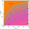 |
Fig. 15. Steady-state OPD from subcooling as a function of Fsky and v for a single ray pass through the wake of a single truss of circumference s = 4.3 m and |

To estimate how the OPD from subcooling scales with telescope size in general, we assume that telescopes of increasing sizes are supported by trusses whose circumference s and length L in the direction parallel to the telescope axis both scale linearly with the primary mirror diameter D, causing the OPD from the wake of each truss to scale like D2. This relationship holds for the structure above the M1 level only, as long as we assume a roughly identical focal ratio of the primary mirrors. However, the tube structure of the upcoming generation of 30-meter-class telescopes and greater is becoming more delicate than that of the preceding 8- to 10-meter-class telescopes: The number of trusses increases, while each truss circumference grows only modestly. In the somewhat unrealistic limit that s does not grow at all and L rises proportionally to D, the OPD scales only linearly with D (but spreads more widely across the pupil). In practice, the scaling power law will lie somewhere in between these extremes.
The rays from a star at center field propagating through a rotationally symmetric telescope travel in a plane defined by the entry point of the ray in the pupil and the optical axis. The closer the entry point is to the central obscuration (CO), the closer the ray segments between reflections are to each other. The air volume that in vertical projection is close to the rim of the CO is therefore traversed at least three times, boosting the OPD on the downwind side of the CO. Unfortunately, the M2 crown and the tertiary mirror tower introduce a lot of vertical surface area in this region with high Fsky. Moreover, any vertically extended tertiary mirror tower and the M2 crown are optically conjugated to a large range of heights above the telescope, which can induce field-dependent errors in the adaptive optics correction. A quantitative analysis requires extensive CFD simulations of the entire dome volume with temperatures (Cho et al. 2011; Vogiatzis et al. 2014, 2018; Ladd et al. 2016; Oser et al. 2018).
3.6. Heat conduction
So far, we have neglected heat conduction within the structures, which will tend to equalize the structure temperature and thus spread the subcooling effect. In Appendix A, we derive the characteristic length scale due to heat conduction ξ with typical values of a few tens of centimeters in telescope trusses (see Table A.1).
The OPD is approximately proportional to  as Eq. (25) shows. Therefore, it is fortunately equivalent to average the temperature around the perimeter of trusses when estimating the OPD in its wake, or for rectangular cross sections for example, to sum the OPD contributions of the four side faces. However, one should not assume that the subcooling spreads evenly along the length of a truss, which typically far exceeds ξ.
3.7. Transient effects
Telescope structures have a significant thermal inertia that delays temperature changes. In Appendix B, we derive the characteristic thermal relaxation timescale τ with typical values of a few hours (see Table A.1).
Sky subcooling is therefore a slow process that generally increases during the night. We note that any incorrect temperature conditioning of the telescope at sunset, including overheating (ΔTsurf > 0), will generate additional OPD, starting already at the beginning of the observations (Wilson 2013).
We point out that in contrast to the characteristic length ξ, the relaxation time τ is linearly dependent on w/h, where w is the truss wall thickness, and thus varies more strongly among different structures in a telescope, even if they are made of the same material. Additionally, the wind veers, the sky temperature drifts, there is variable cloud coverage, the telescope pointing zenith angle varies and so on, and therefore sky subcooling is an inherently transient process and any steady-state computation is only an approximation.
A serious source of wavefront errors in some telescopes is “mirror seeing” (Wilson 2013) caused by ΔTsurf on the optical mirror surface, which can sometimes become even more detrimental than “dome seeing” (Racine et al. 1991). However, mirror seeing is not normally linked to radiative cooling because typical mirrors have broadband coatings, and therefore very low emissivity such as  %. However, subcooling can become a problem if the uncoated backside of a secondary mirror is (partly) exposed to the night sky (the emissivity of typical mirror substrates made of Zerodur® is ≈ 0.9).
To compound the complexity, the ambient air temperature Tamb also fluctuates. During a typical night, Tamb drops quickly after sunset and decreases later more slowly, meaning that the radiation imbalance from the cold sky initially accelerates the thermalization of the telescope. Conversely, a rise in Tamb exacerbates the subcooling. The median temporal gradients of Tamb given in Sect. 2.4 are smaller than typical subcooling gradients of the order of Ṫamb ≈ −1.5 K/τ ≈ −1 K h−1, but are not negligible.
One can shorten the subcooling relaxation time whilst lowering the emissivity and slowing down the structural deflection of the telescope structure by covering the truss surfaces with a thermal insulation layer topped by aluminum foil or thin sheet metal; a strategy chosen at the Subaru Telescope on Mauna Kea, Hawaii (Bely 2006). However, we note that applying an insulation layer on top of a large thermal mass does not diminish the subcooling (i.e., does not mitigate ΔTsurf in the steady state) because the radiation imbalance on its surface is not reduced.
4. Conclusions
Subcooling of structures on the ground is caused by a thermal-radiation imbalance between the night sky and a structure on the ground at ambient temperature which can reach 150 W m−2 and above. Structural elements in telescopes therefore cool by a few Kelvin (see Eqs. (16) and (20)) and in turn cool the surrounding air. Wakes of cooled air flowing from elements in or near the telescope beam, such as spider trusses, the top ring, the tertiary mirror tower, and so on, cause an optical path length difference (OPD), introducing a transient wavefront error. While the size of modern telescopes continues to grow, the budgets of acceptable wavefront error are diminishing for diffraction-limited science cases. Therefore, subcooling poses a serious challenge to the generation of 30-meter telescopes and beyond, and second-generation instruments with adaptive-optics correction in existing 10-meter-class telescopes.
Additionally, we find the following:
-
The integrated thermal sky radiation can be characterized by the effective bolometric sky temperature Tsky. This temperature is dominated by the lower atmosphere and Tsky therefore floats with the ambient air temperature Tamb near the ground. Based on spectra from the Cerro Paranal Sky Model, we derived a simple fit formula for Tsky as a function of Tamb, the PWV column height, and the zenith angle θ; see Eq. (2). The formula is valid for clear sky conditions, which are present at Cerro Paranal for about 90% of the time, and can be applied to any relatively dry site. For the investigated range of PWV values from 0.5 to 20 mm, the difference between Tsky and Tamb varies from −50 K to −25 K for θ = 0°. The discrepancy can decrease by several Kelvin for higher zenith angles.
-
For Cerro Armazones, the site of the ELT, we estimate a median Tsky of about 244 K at a zenith angle of 37°, which lies about 38 K below Tamb.
-
The OPD due to subcooling of a single truss of circumference s is proportional to
 , where
  denotes surface emissivity, Fsky is the sky view factor averaged around the truss cross section, and v is the local air speed; see Eqs. (24) and (25). As large telescopes are generally supported by trusses with both larger circumference and higher (vertical) length, the OPD scales between linearly and quadratically with the primary mirror diameter.
 -
It is crucial to apply low-emissivity coatings to all telescope structures above the primary mirror level that are exposed to a large fraction of the sky. Good choices are either bare aluminum or paints with embedded aluminum particles. On surfaces that may scatter visible stray light, one can apply selective foil that is black in the visible but reflective in the thermal infrared such as Acktar NanoBlack® or Maxorb. Conversely, regular industrial paint usually has high emissivity (
 ), even if it is white.
 -
Sufficient airflow should be maintained in the telescope dome from sunset until the end of the night, for example by opening louvers. Because
 , the wavefront error from subcooling is not just caused by surfaces near the level of the dome slit, but also by any structures closer to the primary mirror if they are poorly ventilated and/or have high emissivity.
 -
Special attention should be devoted to the outer dome cladding because of the combination of high sky view factor (Fsky ≈ 1) and large surface area. It is advisable to use a low-emissivity coating, additionally with low solar absorptivity to limit daytime heating. Again, aluminum alloys or paints with aluminum pigments are good choices, while any colored paints should be avoided.
-
The most critical areas in a telescope structure in terms of wavefront distortion due to subcooling tend to be the vertical ones (i.e., running parallel to the optical axis), in particular surfaces near the projected rim of the central obscuration and the lateral spider truss faces.
-
The ratio of heat capacity to convective efficiency of any telescope structure sets the timescale of thermal relaxation, but these quantities do not influence the steady-state subcooling temperature, as discussed in Sect. 3.7. The time to reach thermal equilibrium can be hours, and therefore subcooling often becomes more serious in the second half of the night.
-
Handheld commercial thermal cameras are not suitable to measure the bolometric sky temperature. These cameras normally use microbolometer detectors (Rogalski 2019), which are only sensitive in the wavelength range of about 8–14 μm which largely overlaps with the astronomical N-band, a region with particularly high atmospheric transmission. On the other hand, if such cameras are employed to estimate subcooling of telescope structures, it is best to take the measurement at the end of the night directly after closing the dome to avoid measuring spuriously low temperatures due to partial sky reflection.
Acknowledgments
W. Kausch is funded by the Hochschulraumstrukturmittel provided by the Austrian Federal Ministry of Education, Science and Research (BMBWF). S. Noll was financed by the project NO 1328/1-1 of the German Research Foundation (DFG). R. Holzlöhner wishes to thank M. Brinkmann (ESO) for stimulating discussions on fluid dynamics and A. Otárola (TMT) for help with the Cerro Armazones environmental data statistics. The authors further thank J. Vinther (ESO) for his continued support of SkyCalc.
References
- Banyal, R. K., & Ravindra, B. 2011, New Astron., 16, 328 [CrossRef] [Google Scholar]
- Bely, P. 2006, The Design and Construction of Large Optical Telescopes (New York: Springer), Astron. Astrophys. Lib. [Google Scholar]
- Berdahl, P., & Fromberg, R. 1982, Sol. Energy, 29, 299 [CrossRef] [Google Scholar]
- Bönsch, G., & Potulski, E. 1998, Metrologia, 35, 133 [NASA ADS] [CrossRef] [Google Scholar]
- Braden, B. 1986, College Math. J., 17, 326 [CrossRef] [Google Scholar]
- Buck, A. L. 1981, J. Appl. Meteorol., 20, 1527 [NASA ADS] [CrossRef] [Google Scholar]
- Chaves, J. 2017, Introduction to Nonimaging Optics (CRC Press) [CrossRef] [Google Scholar]
- Cho, M., Corredor, A., Vogiatzis, K., & Angeli, G. 2011, in Proc. SPIE, eds. T. Andersen, & A. Enmark, Int. Soc. for Opt. and Phot. (SPIE), 8336, 325 [Google Scholar]
- Churchill, S. W., & Bernstein, M. 1977, ASME Trans. J. Heat Trans., 99, 300 [CrossRef] [Google Scholar]
- Clough, S. A., Shephard, M. W., Mlawer, E. J., et al. 2005, J. Quant. Spectr. Rad. Transf., 91, 233 [NASA ADS] [CrossRef] [MathSciNet] [Google Scholar]
- Cullum, M. J., & Spyromilio, J. 2000, in Proc. SPIE, eds. T. Sebring, & T. Andersen, Int. Soc. for Opt. and Phot. (SPIE), 4004, 194 [CrossRef] [Google Scholar]
- Fourier, J. 1822, Théorie Analytique de la Chaleur (Paris: Firmin Didot Pére et Fils), OCLC 2688081 [Google Scholar]
- Gliah, O., Kruczek, B., Etemad, S. G., & Thibault, J. 2011, Heat Mass Trans., 47, 1171 [CrossRef] [Google Scholar]
- Jones, A., Noll, S., Kausch, W., Szyszka, C., & Kimeswenger, S. 2013, A&A, 560, A91 [NASA ADS] [CrossRef] [EDP Sciences] [Google Scholar]
- Kausch, W., Noll, S., Smette, A., et al. 2015, A&A, 576, A78 [NASA ADS] [CrossRef] [EDP Sciences] [Google Scholar]
- Kerber, F., Rose, T., Chacón, A., et al. 2012, Proc. SPIE, 8446, 84463N [CrossRef] [Google Scholar]
- Koehler, B. 2015, E-ELT Environmental Conditions (ESO-191766), Tech. Rep. (Garching, Germany: ESO), (internal document) [Google Scholar]
- Ladd, J., Slotnick, J., Norby, W., Bigelow, B., & Burgett, W. 2016, in Proc. SPIE, eds. G. Z. Angeli, & P. Dierickx, Int. Soc. for Opt. and Phot. (SPIE), 9911, 439 [Google Scholar]
- Lakićević, M., Kimeswenger, S., Noll, S., et al. 2016, A&A, 588, A32 [NASA ADS] [CrossRef] [EDP Sciences] [PubMed] [Google Scholar]
- Li, M., Jiang, Y., & Coimbra, C. F. M. 2017, Sol. Energy, 144, 40 [CrossRef] [Google Scholar]
- Li, M., Liao, Z., & Coimbra, C. F. M. 2018, J. Quant. Spectr. Rad. Transf., 209, 196 [CrossRef] [Google Scholar]
- Lienhard, J. H. 2011, A Heat Transfer Textbook, Dover Books on Engineering (Dover Publications) [Google Scholar]
- Martinez, I. 2020a, Heat and mass convection: Boundary layer flow, http://webserver.dmt.upm.es/~isidoro/bk3/c12/Heatconvection.Boundarylayerflow.pdf [Google Scholar]
- Martinez, I. 2020b, Forced and Natural Convection, http://webserver.dmt.upm.es/~isidoro/bk3/c12/Forcedandnaturalconvection.pdf [Google Scholar]
- Mason, J. J., & Brendel, T. A. 1982, in Optical Coatings for Energy Efficiency and Solar Applications, ed. C. M. Lampert, Int. Soc. Opt. Photonics (SPIE), 0324, 139 [CrossRef] [Google Scholar]
- Milli, J., Kasper, M., Bourget, P., et al. 2018, Proc. SPIE, 10703 [Google Scholar]
- Noll, S., Kausch, W., Barden, M., et al. 2012, A&A, 543, A92 [NASA ADS] [CrossRef] [EDP Sciences] [Google Scholar]
- Oser, M., Ladd, J., Khodadoust, A., Bigelow, B., & Burgett, W. 2018, in Proc. SPIE, eds. G. Z. Angeli, & P. Dierickx, Int. Soc. for Opt. and Phot. (SPIE), 10705, 30 [Google Scholar]
- Otárola, A., Travouillon, T., Schöck, M., et al. 2010, PASP, 122, 470 [NASA ADS] [CrossRef] [Google Scholar]
- Otárola, A., De Breuck, C., Travouillon, T., et al. 2019, PASP, 131, 045001 [NASA ADS] [CrossRef] [Google Scholar]
- Pedrotti, F. L., & Pedrotti, L. S. 1993, Introduction to Optics (Prentice Hall) [Google Scholar]
- Racine, R., Salmon, D., Cowley, D., & Sovka, J. 1991, PASP, 103, 1020 [NASA ADS] [CrossRef] [Google Scholar]
- Rogalski, A. 2019, Infrared and Terahertz Detectors, 3rd edn. (CRC Press) [CrossRef] [Google Scholar]
- Rothman, L. S., Gordon, I. E., Barbe, A., et al. 2009, J. Quant. Spectr. Rad. Transf., 110, 533 [NASA ADS] [CrossRef] [Google Scholar]
- Sarazin, M. 2017, ESO-281474 Document Version 2 [Google Scholar]
- Sauvage, J., Fusco, T., Guesalaga, A., et al. 2015, Adaptive Optics for Extremely Large Telescopes, 1, 4 [Google Scholar]
- Smette, A., Sana, H., Noll, S., et al. 2015, A&A, 576, A77 [NASA ADS] [CrossRef] [EDP Sciences] [Google Scholar]
- Sun, X., Sun, Y., Zhou, Z., Alam, M. A., & Bermel, P. 2017, Nanophotonics, 6, 20 [CrossRef] [Google Scholar]
- Sundén, B., Mander, U., & Brebbia, C. 2010, Advanced Computational Methods and Experiments in Heat Transfer XI, WIT Transactions on Engineering Sciences (WIT Press) [Google Scholar]
- Valencia, J. J., & Quested, P. N. 2010, Metals Process Simulation (ASM International), 18 [Google Scholar]
- Vogiatzis, K., Sadjadpour, A., & Roberts, S. 2014, in Proc. SPIE, eds. G. Z. Angeli, & P. Dierickx, Int. Soc. for Opt. and Phot. (SPIE), 9150, 383 [Google Scholar]
- Vogiatzis, K., Das, K., Angeli, G., Bigelow, B., & Burgett, W. 2018, in Proc. SPIE, eds. G. Angeli, & P. Dierickx, Int. Soc. for Opt. and Phot. (SPIE), 10705, 279 [Google Scholar]
- Wilson, R. 2013, Reflecting Telescope Optics II: Manufacture, Testing, Alignment, Modern Techniques, Astronomy and Astrophysics Library (Springer) [Google Scholar]
- Yarbrough, D. W. 2010, Evaluation of Coatings for Use as Interior RadiationControl Coatings, Tech. Rep. (RIMA, R&D Services, Inc.), https://www.solec.org/wp-content/uploads/2014/02/Evaluation-of-Coatingsfor-Use-as-Interior-Radiation-Control-Coatings-0211.pdf [Google Scholar]
- Yoshii, Y., Aoki, T., Doi, M., et al. 2010, Proc. SPIE, 7733, 773308 [CrossRef] [Google Scholar]
- Zhao, D., Aili, A., Zhai, Y., et al. 2019, Appl. Rev. Phys., 6, 021306 [CrossRef] [Google Scholar]
Appendix A: Heat conduction length scale
We consider a plate and a pipe-shaped truss, both with wall thickness w, letting y be the local surface tangent coordinate along the truss length L and x run along the orthogonal tangential direction. We can write the two-dimensional heat equation for the temperature field u(x, y):=ΔTsurf(x, y) as
![Mathematical equation: $$ \begin{aligned}&-k_m \left( u_{xx} + u_{{ yy}} \right) = q_{\rm sky} - q_{\rm surf} + q_{\rm conv} \\&\;\;\;\; = -\,\frac{h}{{ w}} \left[ \bigl (1 + \eta \bigr )\,u - \eta \,\Delta T_D \right],\nonumber \end{aligned} $$](/articles/aa/full_html/2021/01/aa38853-20/aa38853-20-eq53.gif) (A.1)
(A.1)
where uxx, uyy denote the respective second partial derivatives of u by x and y,  is the specific lateral heat flow per bulk wall volume (unit W m−3) and we have inserted the heat flow terms on the left-hand side of Eq. (12). In Eq. (A.1), we use Eq. (15) where now hrad = hrad(x, y), km is the thermal conductivity of the truss wall material and we assume that the heat conduction normal to the surface is so efficient that the wall becomes isothermal along z, thus u(z) = const and km/w ≫ h.
We define the characteristic length ξ which quantifies the ratio of lateral heat conduction in the truss wall to convection and rewrite Eq. (A.1) as
 (A.2)
(A.2)
 (A.3)
(A.3)
where we assume again hrad ≪ h as discussed after Eq. (15) and the radiative forcing term Urad(x, y) is equal to η ΔTD.
We now consider two different simple structures: The first is a rectangular plate of dimensions L × s × w with L ≫ s ≫ w. We require that there be no heat flux across the plate edges, hence the temperature becomes stationary there. Further, the radiative forcing term contains a step function centered at x = 0, for example because the plate is bent into an L-shaped form with a 90° corner running parallel to the long axis y where the sky view factor changes abruptly:
 (A.4)
(A.4)
where ux is the partial derivative of u by x and sgn(x) = 1 for x > 0, sgn(x) = − 1 for x < 0 and 0 otherwise. The solution of Eq. (A.2) with the boundary conditions in Eq. (A.4) is
![Mathematical equation: $$ \begin{aligned} u(x^\prime ) = \Delta U \left[\tanh \bigl (s^\prime \bigr )\sinh \bigl (x^\prime \bigr ) - \mathrm{sgn}(x) \Bigl ( \cosh \bigl (x^\prime \bigr ) - 1 \Bigr )\right] + U_0, \end{aligned} $$](/articles/aa/full_html/2021/01/aa38853-20/aa38853-20-eq58.gif) (A.5)
(A.5)
where tanh, sinh, and cosh denote the hyperbolic equivalents of the tan, sin, and cos functions, respectively, and we have introduced the reduced variables x′: = x/ξ and s′: = s/(2ξ).
The blue and red curves in Fig. A.1 show u(x), where s = π 0.6 m ≈ 1.88 m, which has the shape of an inverted letter S with its inflection point at (x = 0, u = U0). For this plot we used the material properties of construction steel S355 as listed in Table A.1 and chose w = 10 mm, ΔU = −1 K, and U0 = −2 K. We assumed the two different conductive heat transfer coefficients h1 = 6 W K−1 m−2 and h2 = 3 W K−1 m−2, corresponding to the scaling lengths ξ1 = 0.27 m and ξ2 = 0.39 m (blue and red curves, respectively).
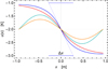 |
Fig. A.1. Example of steady-state temperature distribution u(x) with heat conduction. Blue and red curves: plate of size π 0.6 m with step-like radiative forcing; ξ = 0.27 m and 0.39 m, respectively. Turquoise and orange: same ξ values, but sinusoidal forcing around pipe-shaped truss of diameter d = s/π = 0.6 m. The transition region of the blue curve has the width Δx = 0.55 m. |
Properties of some materials commonly used in telescopes with derived characteristic lengths ξ and relaxation times τ, all for w = 10 mm and h = 4.5 W K−1 m−2.
We can define a transition region width Δx satisfying ux(0) Δx/2 = ΔU, as indicated by the blue dotted line in Fig. A.1. Using ux(0) = ΔU tanh(s′)/ξ, we find
 (A.6)
(A.6)
where the last term is the Taylor expansion about the value s′ = 3 relevant for the presented examples. We conclude that the transition region can cover a significant fraction of a typical steel plate.
The second structure is a pipe-shaped truss of diameter d = s/π with sinusoidal radiative forcing around its circumference instead of the step-like forcing, which could be a model of a vertical truss in the telescope tube, where Fsky peaks on the side facing the telescope axis and becomes minimal on the opposite side oriented towards the inside of the dome. We modify the plate boundary conditions so that the problem becomes periodic in the circumferential coordinate x, as already analyzed by Joseph Fourier (1822)
 (A.7)
(A.7)
where j is any integer. As in the plate problem, Urad(x, y) lies between the extremes U0 + ΔU and U0 − ΔU, which are assumed now at x = 0 and x = ±s/2, respectively. The solution is
 (A.8)
(A.8)
 (A.9)
(A.9)
which is plotted in Fig. A.1 in the turquoise and orange curves for j = 1 and s = 0.6 π m = 1.88 m and again setting ξ1 = 0.27 m and ξ2 = 0.39 m, respectively (as u(x′) is periodic in the pipe case, we have chosen to shift it along x so that its inflection point lies at x = 0 in the plot, as for the plate solution). The factor Ψj compresses the amplitude of the sinusoidal temperature variation around the pipe, in particular if s < 2π j ξ. We note that we can approximate any periodic boundary condition by a Fourier series, hence the linear combination of solutions in Eq. (A.9) with different spatial frequencies j.
If a plate is thermally insulated on one side, such as can be the case for the outer dome cladding, the convective heat exchange on the insulated side is almost turned off. Conversely, for plates whose two side faces are exposed to the ambient air, the interface surface area A is twice that of the insulated case and Fsky should be averaged over the two sides. However, in such a case the average Fsky cannot exceed a value of one-half because of geometric constraints, and therefore the product Fsky A may in some cases not differ strongly from the insulated plate case.
Inside a sealed air-filled structure such as a pipe truss, the enclosed air exchanges heat energy with the internal walls and there is also internal thermal radiation. However, as the internal airflow is usually not forced and because the wall temperature variation is normally too small to induce a significant radiation imbalance, we can neglect these factors.
Summarizing the plate and the pipe examples, we find that u(x) becomes compressed if the characteristic length ξ = (w km/h)1/2 is large compared to s, that is, if lateral conduction dominates over convection. Irrespective of this condition, the average of u(x) around the truss circumference is always equal to the average of Urad, thus U0 = −2 K in our two examples. The limit s ≪ 2π ξ may be referred to as the isothermal regime, while the opposite limit s ≫ 2π ξ may be thought of as thermally disconnected. For a typical telescope pipe steel truss with a wall thickness of w = 10 mm, neither limit clearly applies around its circumference. However, the thermally disconnected regime applies along a typical length L ≫ 2π ξ.
Appendix B: Thermal inertia
Until now, we have discussed only the steady-state solution. We now finally consider the full time-dependent heat equation for a three-dimensional body in air with temperature offset u = u(x, y, z, t):=Tbody(x, y, z, t)−Tamb(t) with time t,
 (B.1)
(B.1)
where cm and ρm are the specific heat capacity and the density of the body material, respectively.
We can consider the pipe problem of the previous section with j = 1 and the initial condition u(x, y, z, 0) = 0 and, setting uzz = Ṫamb = 0, find the solution
 (B.2)
(B.2)
as a function of the reduced time t′ = t/τ with the lateral thermal relaxation time
 (B.3)
(B.3)
We now evaluate the time t = τ after which the term (1 − exp(−t/τ)) grows from zero to 1 − 1/e ≈ 0.63. We assume again the material properties of construction steel S355 listed in Table A.1 and w = 10 mm to arrive at τ1 = 1.64 h and τ2 = 3.27 h for h1 = 6 W K−1 m−2 and h2 = 3 W K−1 m−2, respectively.
Table A.1 shows an overview of some material properties applicable to telescopes. We do not provide an emissivity value for S355 steel since it depends strongly on the surface preparation and regular steel is normally coated anyway to protect from rust. The aluminum alloy 5754 is a candidate for the ELT outer dome cladding ( % corresponds to a clean and 20% to a contaminated surface, respectively).
Zerodur is a low-thermal-expansion glass ceramic used for various telescope mirrors. The thermal conductivity of Zerodur and other glasses and ceramics is often so low that the relation km/w ≫ h no longer holds for mirrors with typical thickness values of w = 50 mm (ELT M1 segments) to hundreds of millimeters. As a consequence, transient thermal phenomena become three-dimensional problems (Banyal & Ravindra 2011) with the relaxation time along z of τz = w2 cm ρm/km.
All Tables
Properties of some materials commonly used in telescopes with derived characteristic lengths ξ and relaxation times τ, all for w = 10 mm and h = 4.5 W K−1 m−2.
All Figures
|
Fig. 1. Sky radiance Lsky(λ) for Cerro Paranal at different PWV conditions typical for observations in the direction of zenith. The astronomical observation bands and the main ozone absorption are marked. For further details on species that are not important for us here (e.g., CO2, N2O and CH4) see Fig. 1 and Table 1 in Smette et al. (2015). |
| In the text | |
|
Fig. 2. Correlation of the sky temperature Tsky and PWV at zenith Only the range of conditions with PWV < 15 mm relevant for typical astronomical observations is used for the final fit function. |
| In the text | |
|
Fig. 3. Correlation of the sky temperature Tsky and zenith distance at a constant level of PWV. |
| In the text | |
|
Fig. 4. Sky radiance at zenith on the coldest and the warmest days at Cerro Paranal (2600m) in July 2018. The fit of a black body is based on the marked points only, defining an upper boundary. |
| In the text | |
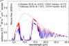 |
Fig. 5. Same as Fig. 4, but for Mauna Kea, Hawaii (4200m) |
| In the text | |
|
Fig. 6. Comparison of the sky temperature |
| In the text | |
|
Fig. 7. Two-dimensional histogram of the ambient temperature Tamb as a function of PWV for clear observing conditions (see text for more details). The bin widths of the histogram are 0.1 mm in PWV and 0.5 K in Tamb. The resulting Pearson coefficient r is indicated (see text for more details). |
| In the text | |
|
Fig. 8. Histogram of the calculated Tsky values; its mean value is 246.2 K, the standard deviation σ = 5.7 K. |
| In the text | |
|
Fig. 9. Tsky vs. TIR at θ = 0° as two-dimensional histogram (bin width of 0.5 K) for clear observing conditions. |
| In the text | |
|
Fig. 10. Evaluation of sky view factors by projection. Red arrow: normal vector n above the point q on a surface. Blue quadrilaterals: two windows of solid angle Ω ≈ 0.16 sr through which the sky can be seen from q (i.e., 𝒯 = 1); the right window is tilted against n by γ = 60°. Green rectangles: projection of the windows onto the tangential plane with areas π Fsky ≈ Ω and Ω × cos(60° ) = Ω/2, respectively. |
| In the text | |
|
Fig. 11. Convective heat transfer coefficient hcyl vs. local air speed v for three different interface lengths s representative of structures in the VLT and ELT telescopes, plus the ELT dome door. |
| In the text | |
|
Fig. 12. Steady-state surface subcooling ΔTsurf as a function of |
| In the text | |
|
Fig. 13. Steady-state surface subcooling ΔTsurf as a function of Fsky and v for s = 4.3 m and |
| In the text | |
|
Fig. 14. Slice through a cylindrical truss of diameter d = s/π running perpendicular to v and to the telescope axis. Red arrow: ray of light traversing the cool wake of thickness δ and temperature difference ΔTwake. |
| In the text | |
|
Fig. 15. Steady-state OPD from subcooling as a function of Fsky and v for a single ray pass through the wake of a single truss of circumference s = 4.3 m and |
| In the text | |
|
Fig. A.1. Example of steady-state temperature distribution u(x) with heat conduction. Blue and red curves: plate of size π 0.6 m with step-like radiative forcing; ξ = 0.27 m and 0.39 m, respectively. Turquoise and orange: same ξ values, but sinusoidal forcing around pipe-shaped truss of diameter d = s/π = 0.6 m. The transition region of the blue curve has the width Δx = 0.55 m. |
| In the text | |
Current usage metrics show cumulative count of Article Views (full-text article views including HTML views, PDF and ePub downloads, according to the available data) and Abstracts Views on Vision4Press platform.
Data correspond to usage on the plateform after 2015. The current usage metrics is available 48-96 hours after online publication and is updated daily on week days.
Initial download of the metrics may take a while.