© ESO 2020

1. Introduction

Black hole seeds with masses of ≳10⁴ M_⊙that are born via direct collapse during the formation process of their host galaxies appear to be a natural explanation for the existence of the most massive black holes observed at high redshift (e.g. Rees 1978, 1984; Volonteri et al. 2008; Woods et al. 2019; Haemmerlé et al. 2020). The direct progenitors of these objects would be supermassive stars (SMSs) growing by accretion at rates of Ṁ > 0.1 M_⊙ yr⁻¹ until they collapse through the general-relativistic (GR) instability (Chandrasekhar 1964). SMSs could form at the centre of protogalaxies in the absence of molecular hydrogen (e.g. Haiman et al. 1997; Omukai 2001; Bromm & Loeb 2003; Dijkstra et al. 2008). Hydrodynamical simulations show that the core of such primordial, atomically cooled haloes would collapse with negligible fragmentation at inflows of 0.1–10 M_⊙ yr⁻¹ below parsec scales (Latif et al. 2013). Another efficient mechanism for the formation of massive black hole seeds is the merger of massive, gas-rich galaxies (Mayer et al. 2010, 2015; Mayer & Bonoli 2019). In addition, to allow for inflows as high as 10⁵ M_⊙ yr⁻¹ at parsec scales, this formation channel does not require primordial chemical composition and metallicities up to solar are expected. Thus, the progenitors of massive black hole seeds could as well be Population I (Pop I) or Population III (Pop III) SMSs.

The evolution of SMSs under rapid accretion has been addressed in several works over the last decade (Begelman 2010; Schleicher et al. 2013; Hosokawa et al. 2013; Sakurai et al. 2015; Umeda et al. 2016; Woods et al. 2017; Haemmerlé et al. 2018a,b, 2019; Haemmerlé & Meynet 2019). For Ṁ ≳ 0.01 M_⊙ yr⁻¹, they evolve as red supergiant protostars (Hosokawa et al. 2013), with most of their mass contained in a radiative envelope (Begelman 2010). As nearly-Eddington stars, their pressure support and entropy content are dominated by radiation to the extent that above a given mass, small post-Newtonian corrections, negligible with regard to the hydrostatic structure, prevent the pressure from restoring the fragile equilibrium against adiabatic perturbations (Chandrasekhar 1964). For Pop III SMSs, the GR instability leads in general to the formation of a black hole seed of nearly the same mass as the progenitor (Fricke 1973; Shapiro & Teukolsky 1979; Uchida et al. 2017), but once metals are included, thermonuclear explosions could prevent black hole formation (Appenzeller & Fricke 1972a,b; Fuller et al. 1986; Montero et al. 2012). Such outcomes depend sensitively on the mass of the SMS at collapse, which is weakly constrained by the models (Woods et al. 2019), especially in the Pop I case.

In a previous work (Haemmerlé 2020), we showed how the onset point of the GR instability can be determined with a high level of accuracy from hydrostatic stellar models. However, the numerical estimates of the final masses suffer from the lack of such models up to the largest masses and accretion rates. The exploration of the parameter space with full stellar evolution is strongly limited by the numerical instability of stellar evolution codes when rapid accretion is included. In the present work, we circumvent this difficulty with the help of simplified analytical hydrostatic structures, built to match the structures obtained with full stellar evolution calculations accounting for rapid accretion. Hylotropes have been proposed by Begelman (2010) to describe the envelope of the “quasi-star” model, where a black hole grows at the centre of an SMS. Numerical models accounting for full stellar evolution showed that this class of structures describes with a high precision the actual envelope of SMSs in the extreme accretion regime (Haemmerlé et al. 2019). Here, we apply the method presented in Haemmerlé (2020) to the full class of hylotropes and discuss the implications regarding the final masses of SMSs in the various versions of direct collapse.

The main properties of rapidly accreting SMSs are reviewed in Sect. 2.1, with an emphasis on the physical motivations for the use of hylotropes. The methods we followed to build the hylotropic models and to determine their stability are described in Sects. 2.2 and 2.3, respectively. The results are presented in Sect. 3 and discussed in Sect. 4. We summarise our conclusions in Sect. 5.

2. Method

2.1. The structure of rapidly accreting SMSs

Relativistic corrections always remain small in SMSs. Considering their equilibrium properties, these stars are well-described by the classical equations of stellar structure (e.g. Hoyle & Fowler 1963; Fuller et al. 1986; Hosokawa et al. 2013; Woods et al. 2017; Haemmerlé et al. 2018a). The equation of state is given by the sum of gas and radiation pressure:

$$\begin{array}{c}\hfill P=\frac{k_{\mathrm{B}}}{\mu m_{\mathrm{H}}}\rho T+\frac{1}{3}{a}_{\mathrm{SB}}{T}^4,\end{array}$$(1)

where P is the total pressure, ρ the mass-density, T the temperature, μm_H the average mass of the free particles of gas, k_B the Boltzmann constant, and a_SB is the Stefan-Boltzmann constant. They are always close to the Eddington limit, with an entropy s_rad given by radiation and a ratio of gas to total pressure of the order of a percent:

$$\begin{array}{c}\hfill \beta :=\frac{P{}_{\mathrm{gas}}}{P}=\frac{1}{1+\frac{\mu m_{\mathrm{H}}}{3k_{\mathrm{B}}}\frac{a_{\mathrm{SB}}{T}^3}{\rho }}=\frac{1}{1+\frac{\mu m_{\mathrm{H}}}{4k_{\mathrm{B}}}s{}_{\mathrm{rad}}}\ll 1.\end{array}$$(2)

Pressure can be expressed as a function of ρ and β:

$$\begin{array}{cc}\hfill P& ={\left(\frac{3}{a_{\mathrm{SB}}}\right)}^{1/3}{\left(\frac{k_{\mathrm{B}}}{\mu m_{\mathrm{H}}}\right)}^{4/3}{\left(\frac{1-\beta }{{\beta }^4}\right)}^{1/3}{\rho }^{4/3}\hfill \\ \hfill \simeq {\left(\frac{3}{a_{\mathrm{SB}}}\right)}^{1/3}{\left(\frac{k_{\mathrm{B}}}{\mu m_{\mathrm{H}}}\right)}^{4/3}{\beta }^{-4/3}{\rho }^{4/3}.\end{array}$$(3)

Due to convection driven by H-burning, the core of an SMS is isentropic (β = cst = :β_c), and therefore, according to Eq. (3), a polytrope of index n = 3:

$$\begin{array}{c}\hfill P=K{\rho }^{4/3},K={\left(\frac{3}{a_{\mathrm{SB}}}\right)}^{1/3}{\left(\frac{k_{\mathrm{B}}}{\mu m_{\mathrm{H}}}\right)}^{4/3}{\left(\frac{1-\beta }{{\beta }^4}\right)}^{1/3}=\mathrm{cst}\end{array}$$(4)

On the other hand, SMSs accrete at rates of Ṁ > 0.1 M_⊙ yr⁻¹, for which the accretion time M/Ṁ is shorter than the thermal timescale (Hosokawa et al. 2013; Haemmerlé et al. 2018a, 2019). As a consequence, the envelope is not thermally relaxed and maintains a higher entropy than the core, inhibiting convection. For rates of Ṁ > 10 M_⊙ yr⁻¹, thermal processes become completely negligible and the radiative envelope evolves adiabatically for most of its mass (Haemmerlé et al. 2019). In this case, the entropy profile builds homologously, which implies the following dependence on the mass coordinate, M_r (r is the radial coordinate):

$$\begin{array}{c}\hfill s\propto \frac{T^3}{\rho }\propto \frac{P^{3/4}}{\rho }\propto {\left(\frac{M_{\mathrm{r}}^2}{r^4}\right)}^{3/4}\frac{r^3}{M_{\mathrm{r}}}=M_{\mathrm{r}}^{1/2}⟹\beta \propto M_{\mathrm{r}}^{-1/2},\end{array}$$(5)

where we used Eq. (2) to express β. With this scaling law, Eq. (3) gives a hylotrope (Begelman 2010):

$$\begin{array}{c}\hfill P=A{M}_{\mathrm{r}}^{2/3}{\rho }^{4/3},\end{array}$$(6)

where A is a constant. The hylotropic law (6) switches into a polytropic law (4) at the limit of the convective core, that is, at a mass coordinate, M_r = M_core. Continuity of pressure at the interface imposes

$$\begin{array}{c}\hfill K=A{M}_{\mathrm{core}}^{2/3}.\end{array}$$(7)

Thus, the structure of a maximally accreting SMS satisfies

$$\begin{array}{cc}\hfill P& =\{\begin{array}{cc}K{\rho }^{4/3}\hfill & \mathrm{if}{M}_{\mathrm{r}}<M_{\mathrm{core}}\hfill \\ K{\left(\frac{M_{\mathrm{r}}}{M_{\mathrm{core}}}\right)}^{2/3}{\rho }^{4/3}\hfill & \mathrm{if}{M}_{\mathrm{r}}>M_{\mathrm{core}}\hfill \end{array},\hfill \end{array}$$(8)

$$\begin{array}{cc}\hfill \beta & =\{\begin{array}{cc}{\beta }_c\hfill & \mathrm{if}{M}_{\mathrm{r}}<M_{\mathrm{core}}\hfill \\ {\beta }_c{\left(\frac{M_{\mathrm{r}}}{M_{\mathrm{core}}}\right)}^{-1/2}\hfill & \mathrm{if}{M}_{\mathrm{r}}>M_{\mathrm{core}}\hfill \end{array},\hfill \end{array}$$(9)

with

$$\begin{array}{c}\hfill K={\left(\frac{3}{a_{\mathrm{SB}}}\right)}^{1/3}{\left(\frac{k_{\mathrm{B}}}{\mu m_{\mathrm{H}}}\right)}^{4/3}{\left(\frac{1-{\beta }_c}{{\beta }_c^4}\right)}^{1/3}.\end{array}$$(10)

The entropy profiles of the GENEC models of Haemmerlé et al. (2018a, 2019) at zero metallicity and Ṁ = 1 − 1000 M_⊙ yr⁻¹ are shown in Figs. 1–4. These profiles are similar in all respects to those found with other codes (Hosokawa et al. 2013; Umeda et al. 2016). The limit between the polytropic, convective core, and the hylotropic, radiative envelope appears clearly. An additional feature is visible, namely, the nearly vertical outer end of the profiles. The layers that are newly accreted gain entropy as they are incorporated in the stellar interior, which triggers convection. However, this impacts only the outer percent of the stellar mass, where the density is the lowest, and this feature can be neglected for our purpose. We see that for rates of Ṁ ≥ 100 M_⊙ yr⁻¹ the successive entropy profiles match each other in the envelope, following the hylotropic law (5). For 10 M_⊙ yr⁻¹, the external layers depart slightly from the hylotropic law. For lower rates, the hylotropic approximation is broken in the whole envelope.

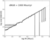Fig. 1. Entropy profiles of the GENEC model at zero metallicity and Ṁ = 1000 M⊙ yr−1, at masses of M = 1−2 − 3−4 − 5 × 105 M⊙. The grey dotted line indicates the power-law $s=1.82\frac{k_{\text{B}}}{m_{\text{H}}}{(M_{\mathrm{r}}/M_{\odot })}^{1/2}$.

Fig. 2. Same as in Fig. 1 for Ṁ = 100 M⊙ yr−1 and M = 1−2 − 3−4 × 105 M⊙.

Fig. 3. Same as in Fig. 1 for Ṁ = 10 M⊙ yr−1 and M = 1−2 − 3−4 − 5 × 105 M⊙.

Fig. 4. Same as in Fig. 1 for Ṁ = 1 M⊙ yr−1 and M = 0.1−0.3−1 − 2 × 105 M⊙.

2.2. Hylotropic structures

Provided a constraint on pressure P = f(ρ, M_r), classical spherical stellar structures are fully determined by hydrostatic equilibrium and continuity of mass:

$$\begin{array}{cc}& \frac{\mathrm{d}P}{\mathrm{d}r}=-\rho \frac{G{M}_{\mathrm{r}}}{r^2},\hfill \end{array}$$(11)

$$\begin{array}{cc}\hfill & \frac{\mathrm{d}{M}_r}{\mathrm{d}r}=4\pi r^2\rho ,\hfill \end{array}$$(12)

where G is the gravitational constant. We introduce the dimensionless functions ξ, θ, φ and ψ:

$$\begin{array}{c}\hfill \xi =\alpha r,\rho ={\rho }_c{\theta }^3,\phi =\frac{{\alpha }^3}{4\pi {\rho }_c}{M}_{\mathrm{r}},P=P_c\psi ,\end{array}$$(13)

where ρ_c and P_c are the central mass-density and pressure, and α is related to them by

$$\begin{array}{c}\hfill {\alpha }^2=\frac{\pi G{\rho }_c^2}{P_c}.\end{array}$$(14)

The boundary conditions are given by

$$\begin{array}{ccc}\hfill r=0& :\hfill & \hfill \xi =0,\theta =\psi =1,\phi =0,\end{array}$$(15)

$$\begin{array}{ccc}\hfill r=R& :\hfill & \hfill \xi =\alpha R=:{\xi }_{\mathrm{surf}},\theta =\psi =0,\phi =\frac{{\alpha }^{3}M}{4\pi {\rho }_c}=:{\phi }_{\mathrm{surf}},\\ \hfill \end{array}$$(16)

where M and R are the total mass and radius of the star, with φ_surf and ξ_surf as their dimensionless equivalents. With these dimensionless functions, Eqs. (11)–(12) become

$$\begin{array}{cc}\hfill \frac{\mathrm{d}\psi }{\mathrm{d}\xi }& =-4\frac{\phi {\theta }^3}{{\xi }^2},\hfill \end{array}$$(17)

$$\begin{array}{cc}\hfill \frac{\mathrm{d}\phi }{\mathrm{d}\xi }& ={\xi }^2{\theta }^3.\hfill \end{array}$$(18)

The constraint on pressure reduces to a function ψ(θ, φ) that closes Eqs. (17)–(18). Translated into the dimensionless functions (13), Eqs. (8)–(9) give

$$\begin{array}{c}\hfill \psi =\{\begin{array}{cc}{\theta }^4\hfill & \mathrm{if}\phi <{\phi }_{\mathrm{core}}\hfill \\ {\left(\frac{\phi }{{\phi }_{\mathrm{core}}}\right)}^{2/3}{\theta }^4\hfill & \mathrm{if}\phi >{\phi }_{\mathrm{core}}\hfill \end{array},\end{array}$$(19)

$$\begin{array}{c}\hfill \beta =\{\begin{array}{cc}{\beta }_c\hfill & \mathrm{if}\phi <{\phi }_{\mathrm{core}}\hfill \\ {\beta }_c{\left(\frac{\phi }{{\phi }_{\mathrm{core}}}\right)}^{-1/2}\hfill & \mathrm{if}\phi >{\phi }_{\mathrm{core}}\hfill \end{array},\end{array}$$(20)

where

$$\begin{array}{c}\hfill {\phi }_{\mathrm{core}}:=\frac{{\alpha }^3}{4\pi {\rho }_c}{M}_{\mathrm{core}}\end{array}$$(21)

is the dimensionless mass of the convective core which remains the only free parameter in the equation system.

Hylotropic structures can be built by numerical integration of (17)–(18) with constraint (19), starting from central conditions (15). For the numerical integration of the hylotropic envelope (φ >  φ_core), we follow the more suitable Lagrangian formulation of Begelman (2010) who defines w = dlnξ/dlnφ. In terms of this variable, Eqs. (11)–(12) with (6) lead to

$$\begin{array}{cc}\hfill \frac{\mathrm{dln}\phi }{\mathrm{dln}w}& =\frac{1}{\frac{3}{2}-3w+3{\phi }_{\mathrm{core}}^{2/3}{w}^{4/3}},\hfill \end{array}$$(22)

$$\begin{array}{cc}\hfill \frac{\mathrm{dln}\xi }{\mathrm{dln}w}& =\frac{w}{\frac{3}{2}-3w+3{\phi }_{\mathrm{core}}^{2/3}{w}^{4/3}}.\hfill \end{array}$$(23)

The functions θ, ψ and β are then obtained by Eqs. (18)–(20). Since w → ∞ when ρ → 0, integration with respect to w never reaches the surface. We stop the integration when θ <  10⁻⁸. We build in this way a series of hylotropes with φ_core ranging in the interval:

$$\begin{array}{c}\hfill {\phi }_{\min }:=0.459<{\phi }_{\mathrm{core}}<2.02=:{\phi }_{\max }\end{array}$$(24)

by steps of 0.05–0.3. The lower limit of this interval is imposed by the condition of gravitational binding (Begelman 2010), while the upper limit corresponds to polytropes, that is, φ_core = φ_surf.

The dimensional quantities can then be derived from the dimensionless ones. The polytropic law (4) in the core implies $P_c=K{\rho }_c^{4/3}$. With the definition (14) of α and the expression (10) of K, it gives a mass scale of

$$\begin{array}{c}\hfill \frac{4\pi {\rho }_c}{{\alpha }^3}=\frac{4}{\sqrt{\pi }}{\left(\frac{K}{G}\right)}^{3/2}=\frac{4}{G^{3/2}}{\left(\frac{3}{\pi a_{\mathrm{SB}}}\right)}^{1/2}{\left(\frac{k_{\mathrm{B}}}{\mu m_{\mathrm{H}}}\right)}^2{\left(\frac{1-{\beta }_c}{{\beta }_c^4}\right)}^{1/2}.\end{array}$$(25)

We see that the mass scale is fully determined by β_c and the chemical composition. The choice of the central temperature, imposed by H-burning, determines ρ_c via Eq. (2), which defines the length-scale α⁻¹ through the mass scale (25).

2.3. GR instability in the post-Newtonian + Eddington limit

We showed in Haemmerlé (2020) that the onset point of the GR instability can be determined with high accuracy from numerical hydrostatic structures by a simple application of the relativisitic equation of adiabatic pulsation of Chandrasekhar (1964) in the following form:

$$\begin{array}{c}\hfill \frac{{\omega }^2}{c^2}{I}_0={\displaystyle \sum _{i=1}^4{I}_i}\end{array}$$(26)

with

$$\begin{array}{cc}\hfill I_0& ={\displaystyle {\int }_0^R{e}^{a+3b}(P+\rho c^2)r^4\mathrm{d}r,}\hfill \end{array}$$(27)

$$\begin{array}{cc}\hfill I_1& =9{\displaystyle {\int }_0^R{e}^{3a+b}({\mathrm{\Gamma }}_1-\frac{4}{3})P{r}^2\mathrm{d}r,}\hfill \end{array}$$(28)

$$\begin{array}{cc}\hfill I_2& =-12{\displaystyle {\int }_0^R{e}^{3a+b}(a^{\prime }+\frac{b^{\prime }}{3})P{r}^3\mathrm{d}r,}\hfill \end{array}$$(29)

$$\begin{array}{cc}\hfill I_3& =\frac{8\pi G}{c^4}{\displaystyle {\int }_0^R{e}^{3(a+b)}P(P+\rho c^2)r^4\mathrm{d}r,}\hfill \end{array}$$(30)

$$\begin{array}{cc}\hfill I_4& =-{\displaystyle {\int }_0^R{e}^{3a+b}\frac{P^{\prime 2}}{P+\rho c^2}{r}^4\mathrm{d}r,}\hfill \end{array}$$(31)

where ′ indicates the derivatives with respect to the radial coordinate r (r = R at the surface), P is the pressure, ρ the density of relativistic mass, c the speed of light, G the gravitational constant, Γ₁ the first adiabatic exponent, and a and b are the coefficients of the metric:

$$\begin{array}{c}\hfill {\mathrm{d}s}^2=-e^{2a}{(c\mathrm{d}t)}^2+e^{2b}{\mathrm{d}r}^2+r^2\mathrm{d}{\mathrm{\Omega }}^2.\end{array}$$(32)

Einstein’s equations lead to the following expressions for a spherical, static metric:

$$\begin{array}{cc}& a^{\prime }=\frac{G{M}_{\mathrm{r}}}{r^2{c}^2}\frac{1+\frac{4\pi r^3}{M_{\mathrm{r}}{c}^2}P}{1-\frac{2G{M}_{\mathrm{r}}}{r{c}^2}},e^{2a(R)}=1-\frac{2GM}{R{c}^2},\hfill \end{array}$$(33)

$$\begin{array}{cc}\hfill & e^{-2b}=1-\frac{2G{M}_{\mathrm{r}}}{r{c}^2}.\hfill \end{array}$$(34)

The relativistic mass-coordinates M_r (M = M_R) is related to the other quantities by Eq. (12) with relativistic-mass instead of rest-mass in M_r and ρ.

The condition for GR instability is

$$\begin{array}{c}\hfill {\displaystyle \sum _{i=1}^4{I}_i<0.}\end{array}$$(35)

Here, we formulate this condition for the special case of post-Newtonian stars near the Eddington limit. To that aim, we re-express integrals I_i in the dimensionless functions (13). Following Tooper (1964a), we also define:

$$\begin{array}{c}\hfill \sigma :=\frac{P_c}{{\rho }_c{c}^2}=\frac{\pi G{\rho }_c}{{\alpha }^2{c}^2},\end{array}$$(36)

which represents the dimensionless parameter for the relativistic correction since compactness is given by

$$\begin{array}{c}\hfill \frac{2G{M}_{\mathrm{r}}}{r{c}^2}=8\sigma \frac{\phi }{\xi }.\end{array}$$(37)

In these dimensionless quantities, integrals (28)–(31) are given as:

$$\begin{array}{cc}\hfill I_1& =9\frac{P_c}{{\alpha }^3}{\displaystyle \int }{e}^{3a+b}({\mathrm{\Gamma }}_1-\frac{4}{3})\psi {\xi }^2\mathrm{d}\xi ,\hfill \end{array}$$(38)

$$\begin{array}{cc}\hfill I_2& =-12\frac{P_c}{{\alpha }^3}{\displaystyle \int }{e}^{3a+b}(\frac{\mathrm{d}a}{\mathrm{d}\xi }+\frac{1}{3}\frac{\mathrm{d}b}{\mathrm{d}\xi })\psi {\xi }^3\mathrm{d}\xi ,\hfill \end{array}$$(39)

$$\begin{array}{cc}\hfill I_3& =8\sigma \frac{P_c}{{\alpha }^3}{\displaystyle \int }{e}^{3(a+b)}(1+\sigma \frac{\psi }{{\theta }^3})\psi {\theta }^3{\xi }^4\mathrm{d}\xi ,,\hfill \end{array}$$(40)

$$\begin{array}{cc}\hfill I_4& =-\sigma \frac{P_c}{{\alpha }^3}{\displaystyle \int }{e}^{3a+b}\frac{{\left(\frac{\mathrm{d}\psi }{\mathrm{d}\xi }\right)}^2}{1+\sigma \frac{\psi }{{\theta }^3}}\frac{{\xi }^4\mathrm{d}\xi }{{\theta }^3},\hfill \end{array}$$(41)

where the integration is made over the interval 0 <  ξ <  ξ_surf. Each integral has the same dimensional factor P_c/α³ in front, which can be extracted from the sum and cancelled via the inequality (35).

In the Eddington limit, the ratio of gas to total pressure is β ≪ 1 and the first adiabatic exponent can be evaluated as

$$\begin{array}{c}\hfill {\mathrm{\Gamma }}_1=\frac{4}{3}+\frac{\beta }{6}=\frac{4}{3}+\frac{{\beta }_{\mathrm{c}}}{6}\frac{\beta }{{\beta }_c}.\end{array}$$(42)

We take the central value β_c ≪ 1 as the parameter for the departures from the Eddington limit, such as σ ≪ 1 represents the departures from the Newtonian limit. For post-Newtonian stars near the Eddington limit, integrals (38)–(41)) can be developed in these two parameters, neglecting second-order terms, 𝒪(σ²) or 𝒪(β_cσ). We notice that with the previously used Eq. (42), each integral has a global σ or β_c factor, except for I₂, where the σ factor has to be extracted from the derivatives of the metric. These derivatives are taken from Eqs. (33)–(34) and we only need the 𝒪(σ) terms:

$$\begin{array}{cc}\hfill \frac{\mathrm{d}a}{\mathrm{d}\xi }& =4\sigma \frac{\phi }{{\xi }^2},\hfill \end{array}$$(43)

$$\begin{array}{cc}\hfill \frac{\mathrm{d}b}{\mathrm{d}\xi }& =-4\sigma \frac{\phi }{{\xi }^2}+4\sigma \xi {\theta }^3,\hfill \end{array}$$(44)

(using Eq. (18)). In this way, each integral has either a global σ or β_c factor, which makes all the other relativistic corrections useless. In particular, we can ignore all other departures from Minkowskian metric and take e^3a + b = e^3(a + b) = 1. Finally, the pressure gradient in I₄ can be eliminated with classical hydrostatic equilibrium (17). Once we remove all the second-order terms, the integrals read:

$$\begin{array}{cc}\hfill I_1& =\frac{3}{2}{\beta }_c\frac{P_c}{{\alpha }^3}{\displaystyle \int }\frac{\beta }{{\beta }_c}\psi {\xi }^2\mathrm{d}\xi ,\hfill \end{array}$$(45)

$$\begin{array}{cc}\hfill I_2& =-16\sigma \frac{P_c}{{\alpha }^3}{\displaystyle \int }(\xi {\theta }^3+\frac{2\phi }{{\xi }^2})\psi {\xi }^3\mathrm{d}\xi ,\hfill \end{array}$$(46)

$$\begin{array}{cc}\hfill I_3& =8\sigma \frac{P_c}{{\alpha }^3}{\displaystyle \int }\psi {\theta }^3{\xi }^4\mathrm{d}\xi ,\hfill \end{array}$$(47)

$$\begin{array}{cc}\hfill I_4& =-16\sigma \frac{P_c}{{\alpha }^3}{\displaystyle \int }{\phi }^2{\theta }^3\mathrm{d}\xi ,\hfill \end{array}$$(48)

and their sum is

$$\begin{array}{cc}& \frac{2{\alpha }^3}{3P_c}{\displaystyle \sum _{i=1}^4}{I}_i={\beta }_c\int \frac{\beta }{{\beta }_c}\psi {\xi }^2\mathrm{d}\xi \hfill \end{array}$$(49)

$$\begin{array}{cc}\hfill & -\frac{16}{3}\sigma ({\displaystyle \int }{\xi }^4\psi {\theta }^3\mathrm{d}\xi +2{\displaystyle \int }{\phi }^2{\theta }^3\mathrm{d}\xi \hfill \end{array}$$(50)

$$\begin{array}{cc}\hfill & +4{\displaystyle \int \xi \psi \phi }\mathrm{d}\xi ).\hfill \end{array}$$(51)

The first integral in the σ term can be expressed as a function of the other two, using (i) the continuity Eq. (18), (ii) an integration by parts (boundary terms vanish), (iii) hydrostatic equilibrium (17):

$$\begin{array}{c}\hfill {\displaystyle \int }{\xi }^4\psi {\theta }^3\mathrm{d}\xi \stackrel{(\mathrm{i})}{=}{\displaystyle \int }{\xi }^2\psi \frac{\mathrm{d}\phi }{\mathrm{d}\xi }\mathrm{d}\xi \stackrel{(\mathrm{ii})}{=}-{\displaystyle \int }\phi \frac{\mathrm{d}}{\mathrm{d}\xi }\left({\xi }^2\psi \right)\mathrm{d}\xi \end{array}$$(52)

$$\begin{array}{c}\hfill \stackrel{(\mathrm{iii})}{=}-2{\displaystyle \int }\xi \psi \phi \mathrm{d}\xi +4{\displaystyle \int }{\phi }^2{\theta }^3\mathrm{d}\xi .\end{array}$$(53)

As a consequence, the GR instability occurs when

$$\begin{array}{c}\hfill \frac{{\beta }_c}{\sigma }<\frac{32}{3}\frac{\int \xi \psi \phi \mathrm{d}\xi +3\int {\phi }^2{\theta }^3\mathrm{d}\xi }{\int \frac{\beta }{{\beta }_c}\psi {\xi }^2\mathrm{d}\xi }=:{\frac{\beta }{\sigma }|}_{\mathrm{crit}}.\end{array}$$(54)

Since we extracted already the post-Newtonian correction through σ, the integrals in Eq. (54) can be evaluated numerically from Newtonian structures (σ → 0), either numerical or analytical. Departures from the Eddington limit are already included in the factor β_c and the function β/β_c, that is, by the effect of gas pressure and we do not need to account for corrections due to the entropy of gas, which justifies a choice of the index, namely, n = 3, in the core (Sect. 2.1). Thus, it allows us to consistently capture the GR instability on the classical hylotropic models displayed in Sect. 2.2. Distinctions between relativistic- and rest-mass in the hydrostatic structures are insignficant.

For given dimensionless structures, determined by the functions θ(ξ), φ(ξ), ψ(ξ), and β(ξ)/β_c, Eq. (54) gives a critical ratio of β_c and σ. On the other hand, by definition of β_c (1)–(2) and σ (36), the actual product of these two quantities is directly given by the central temperature, T_c, and the chemical composition:

$$\begin{array}{c}\hfill {\beta }_c\sigma =\frac{k_{\mathrm{B}}{T}_{\mathrm{c}}}{\mu m_{\mathrm{H}}{c}^2}.\end{array}$$(55)

Thus, for given dimensionless structures, the properties of the star at the limit of stability are fully determined by central temperature and chemical composition, since β_c and σ are both defined.

3. Results

From the full series of hylotropic structures built according to Sect. (2.2), three of them are shown in Fig. 5, together with the polytrope. As noted by Begelman (2010), a decrease in φ_core translates into an increase in φ_surf, the total dimensionless mass. This is because the pressure gradient is flatter with the hylotropic law than with the polytropic one due to the dependence on the mass coordinate. Thus, larger masses are reached before pressure and density vanish. To show this effect more clearly, we plot φ_surf as a function of φ_core for the full series of structures in Fig. 6 (we note the logarithmic scale in the y-axis). The increase remains moderate down to φ_core ≳ 1, but then φ_surf gains orders of magnitude to reach millions when φ_core → φ_min. The mass fraction of the core as a function of ξ_core in Begelman (2010) is well-reproduced by our series of structures.

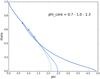Fig. 5. Hylotropic structures built according to Sect. 2.2, for the indicated values of φcore, the dimensionless mass of the core. The dotted line is the polytrope used for the core and a circle indicates φcore for the various models.

For this series of structures, we inject the functions θ(ξ), φ(ξ), ψ(ξ), and β(ξ)/β_c from Eqs. 19–(20) into the stability condition (54). It gives the critical ratio ${\frac{\beta }{\sigma }|}_{\mathrm{crit}}$ as a function of φ_core, which is shown in Fig. 7. In the polytropic limit φ_core → φ_max, we find a value 15.8 that reproduces the numerical tables of Chandrasekhar (1964) and Tooper (1964b) well. When φ_core <  φ_surf, the critical ratio departs towards larger values. It could be interpreted naively as a destabilising effect, but it reflects only the increase in φ_surf that results from the decrease in φ_core. In other words, we compare objects of different masses. We can see already that when the total dimensionless mass gains several orders of magnitude (Fig. 6), the critical ratio ${\frac{\beta }{\sigma }|}_{\mathrm{crit}}$ grows only by a factor of a few, which suggests that hylotropes with low φ_core remain stable up to larger masses than polytropes.

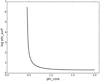Fig. 6. Total dimensionless mass as a function of the dimensionless mass of the core for the series of hylotropic structures built according to Sect. 2.2.

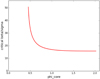Fig. 7. Critical ratio ${\frac{\beta }{\sigma }|}_{\mathrm{crit}}$ of Eq. (54) for the series of hylotropic structures built according to the steps detailed in Sect. 2.2.

In order to quantify this effect, we fix the product, β_cσ, according to Eq. (55), and impose critical conditions ${\beta }_c/\sigma ={\frac{\beta }{\sigma }|}_{\text{crit}}$. The central temperature of Pop III SMSs is always comprised in the interval 1.5−2 × 10⁸ K and the chemical composition does not depart significantly from μ = 0.6 (Hosokawa et al. 2013; Haemmerlé et al. 2018a). With these values in Eq. (55) and the critical condition, β_c, is determined, which gives the mass-scale via Eq. (25). This allows us to express the mass of the star and that of the core in solar units.

The result of this treatment is shown in Fig. 8. We see that the changes in central temperature over the narrow range of relevant values does not change the stability limit significantly. For polytropic structures, the maximum mass consistant with stability is 1−1.5 × 10⁵ M_⊙, which is in agreement with Woods et al. (2020). However, when the mass fraction of the convective core decreases, we see that the limit of stability moves towards larger masses. In other words, the hylotropic law in the envelope has a stabilising effect against adiabatic pulsations as it decreases the compactness. The effect becomes extremely strong when the mass of the core stays as low as ∼10⁴ M_⊙. In this case, masses in excess of 10⁶ M_⊙ could be reached, resulting from the sensitive dependence of the total mass on the core mass when φ_core <  1, while the critical ratio ${\frac{\beta }{\sigma }|}_{\mathrm{crit}}$ does not change much, as noted above. Thus, the mass of the convective core appears as a key quantity and a star hardly reaches instability if its convective core does not exceed ∼10⁴ M_⊙. It is only for total masses of ≳10⁷ M_⊙ (not shown in the figure) that the stability limit moves to M_core <  10⁴ M_⊙. At the limit of gravitational binding (φ_core → φ_min, Eq. (24)), we obtain the largest mass consistant with stable equilibrium, which is ∼5 × 10¹⁰ M_⊙, with a core of ∼5000 M_⊙ (i.e. a core mass fraction of 10⁻⁷).

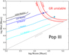Fig. 8. Total mass of the star versus mass of the convective core in the Pop III case. Solid red lines indicate the limit of stability for hylotropic models with μ = 0.6 and Tc = 1.5−2 × 108 K. The GENEC models of Haemmerlé et al. (2018a, 2019) at zero metallicity are plotted with the indicated rates. The identity corresponds to polytropes of different masses, and is shown as a grey line. The final masses obtained in Haemmerlé (2020) are marked by star-like symbols. The dotted red line is the limit of stability for hylotropes with μ = 0.6 and the exact central temperature of the GENEC model at 10 M⊙ yr−1 at the onset of instability (Tc = 1.78 × 108 K).

In the Pop I case, shown in Fig. 9, the lower central temperatures shift the stability limit towards higher masses, allowing it to reach ∼3−5 × 10⁵ M_⊙ in the polytropic limit. At the same time, the typical core’s mass required for GR instability moves up to ∼3−5 × 10⁴ M_⊙.

Fig. 9. Same as in Fig. 8 in the Pop I case.

4. Discussion

The reliability of the hylotropic models can be tested by a comparison with the results of the GENEC models (Haemmerlé et al. 2018a, 2019; Haemmerlé 2020). The entropy profiles of these models suggest that hylotropes are relevant for rates of ≳100 M_⊙ yr⁻¹ (Sect. 2.1). The GENEC tracks are displayed in Fig. 8 for zero metallicity, with their collapse points indicated as star-like symbols. The comparison can be made only for 1 and 10 M_⊙ yr⁻¹since the other models are still a substantial distance from any instability. We see that the last stable model at 10 M_⊙ yr⁻¹ lies in the critical band of hylotropic models with T_c = 1.5−2 × 10⁸ K, while the one at 1 M_⊙ yr⁻¹ goes slightly over the limit. To refine the comparison, we plot as a red dotted line the hylotropic limit with the exact central temperature of the GENEC model at 10 M_⊙ yr⁻¹ at the onset point of instability (T_c = 1.78 × 10⁸ K). We see that the matching is perfect. Departures from hylotropy in the entropy profile of this model (Fig. 3) occur only near the surface, where the density is low, which implies negligible changes in the GR corrections. It is only for rates of ≤1 M_⊙ yr⁻¹ that the entropy profiles depart from hylotropy in the inner envelope (Fig. 4). We note that the central temperature of the last stable model at 1 M_⊙ yr⁻¹ is very close to 1.5 × 10⁸ K, so that the upper red curve gives the hylotropic limit relevant for this model. Thus, even at this rate, the hylotropic limit is only exceeded by ∼0.1 dex in the (M, M_core) diagram. An extrapolation of the curve at 0.1 M_⊙ yr⁻¹ suggests that this model, if it ever reaches the GR instability during H-burning, does so as a fully relaxed, polytropic star. Overall, it appears difficult to find a rate for which the hylotropic limit would be significantly exceeded. For rates of > 1000 M_⊙ yr⁻¹, an extrapolation of the tracks suggests final masses in excess of 10⁶ M_⊙.

The GENEC tracks at solar metallicity are plotted in Fig. 9 for the two available rates, namely, 1 and 1000 M_⊙ yr⁻¹. The central temperatures that have been used for the hylotropic models correspond to that of the last stable structure of the 1000 M_⊙ yr⁻¹ run (8.5 × 10⁷ K) and of the last model of the 1 M_⊙ yr⁻¹ run (6 × 10⁷ K), which is still far from instability. We see that the larger convective core of Pop I models cancels the effect of the lower central temperature, as the tracks are shifted with the stability limit. As expected, the stability limit given by the hylotropic models with the relevant central temperature crosses the 1000 M_⊙ yr⁻¹ track at the exact point of instability obtained in Haemmerlé (2020), which corresponds to a mass of 759 000 M_⊙. The comparison cannot be done for lower rates due to the lack of models. As in the Pop III case, masses of > 10⁶ M_⊙ require rates of > 1000 M_⊙ yr⁻¹.

These results confirm that spherical SMSs forming in atomically cooled haloes cannot reach masses in excess of 500 000 M_⊙, while masses in excess of 10⁶ M_⊙ could be reached in the galaxy merger scenario (see Sect. 1), provided accretion rates of ≳1000 M_⊙ yr⁻¹. In fact, such rates appear necessary for massive black hole formation through Pop I galaxy mergers since at solar metallicity, masses of ≳10⁶ M_⊙ are required to avoid thermonuclear explosion during the collapse (Montero et al. 2012). In this respect, the final mass of the black hole progenitor ranges across distinct intervals throughout the various versions of direct collapse: ≲500 000 M_⊙ for atomically cooled haloes; this value is ≳10⁶ M_⊙ for Pop I galaxy mergers.

We note that this picture could change significantly when including rotation. Given enough angular momentum, the centrifugal force has been shown to remove the GR instability in polytropic models up to masses of ∼10⁸ M_⊙ (Fowler 1966; Bisnovatyi-Kogan et al. 1967). On the other hand, rapidly accreting SMSs must be slow rotators (Haemmerlé et al. 2018b) due to the ΩΓ-limit (Maeder & Meynet 2000). For masses of > 10⁵ M_⊙, their surface velocity cannot exceed a few percents of the Keplerian velocity. The impact of rotation on the stability of hylotropic models shall be addressed in a forthcoming work.

5. Summary and conclusions

In this work, we estimate the final masses of the progenitors of massive black hole seeds in the various versions of direct collapse on the basis of hylotropic models built according to Begelman (2010). Through a comparison with the GENEC models, accounting for full stellar evolution (Haemmerlé et al. 2018a, 2019; Haemmerlé 2020), we show that hylotropic models are able to predict the final masses with a high level of accuracy for accretion rates of ≥10 M_⊙ yr⁻¹ and it remains a very good approximation even for lower rates.

The hylotropic law in the envelope has a stabilising effect against adiabatic perturbations to equilibrium as it decreases the compactness and, thus, reduces the destabilising GR effects. The mass of the convective core is consequential for the stability of the star. The lower the core’s mass, the larger the total mass consistent with stable equilibrium (Figs. 8–9). Typical conditions for GR instability are a total mass ≳10⁵ M_⊙ with a core mass ≳10⁴ M_⊙. For a core mass as low as ≲10⁴ M_⊙, total masses in excess of 10⁶ − 10⁷ M_⊙ remain consistent with stability.

These results confirm that spherical SMSs forming in atomically cooled haloes (Pop III, Ṁ ≲ 10 M_⊙ yr⁻¹) have masses of ≲500 000 M_⊙. With regard to SMSs formed by accretion at rates of ≳1000 M_⊙ yr⁻¹, these could reach masses of ≳10⁶ M_⊙, which is a required condition for massive black hole formation in Pop I galaxy mergers. It implies that the final masses of the progenitors of massive black hole seeds range across distinct intervals throughout the various versions of direct collapse.

Acknowledgments

LH has received funding from the European Research Council (ERC) under the European Union’s Horizon 2020 research and innovation programme (grant agreement No 833925, project STAREX).

References

All Figures

	Fig. 1. Entropy profiles of the GENEC model at zero metallicity and Ṁ = 1000 M⊙ yr−1, at masses of M = 1−2 − 3−4 − 5 × 105 M⊙. The grey dotted line indicates the power-law $s=1.82\frac{k_{\text{B}}}{m_{\text{H}}}{(M_{\mathrm{r}}/M_{\odot })}^{1/2}$.
In the text

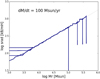	Fig. 2. Same as in Fig. 1 for Ṁ = 100 M⊙ yr−1 and M = 1−2 − 3−4 × 105 M⊙.
In the text

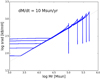	Fig. 3. Same as in Fig. 1 for Ṁ = 10 M⊙ yr−1 and M = 1−2 − 3−4 − 5 × 105 M⊙.
In the text

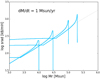	Fig. 4. Same as in Fig. 1 for Ṁ = 1 M⊙ yr−1 and M = 0.1−0.3−1 − 2 × 105 M⊙.
In the text

	Fig. 5. Hylotropic structures built according to Sect. 2.2, for the indicated values of φcore, the dimensionless mass of the core. The dotted line is the polytrope used for the core and a circle indicates φcore for the various models.
In the text

	Fig. 6. Total dimensionless mass as a function of the dimensionless mass of the core for the series of hylotropic structures built according to Sect. 2.2.
In the text

	Fig. 7. Critical ratio ${\frac{\beta }{\sigma }|}_{\mathrm{crit}}$ of Eq. (54) for the series of hylotropic structures built according to the steps detailed in Sect. 2.2.
In the text

Fig. 8. Total mass of the star versus mass of the convective core in the Pop III case. Solid red lines indicate the limit of stability for hylotropic models with μ = 0.6 and Tc = 1.5−2 × 108 K. The GENEC models of Haemmerlé et al. (2018a, 2019) at zero metallicity are plotted with the indicated rates. The identity corresponds to polytropes of different masses, and is shown as a grey line. The final masses obtained in Haemmerlé (2020) are marked by star-like symbols. The dotted red line is the limit of stability for hylotropes with μ = 0.6 and the exact central temperature of the GENEC model at 10 M⊙ yr−1 at the onset of instability (Tc = 1.78 × 108 K).

In the text

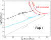	Fig. 9. Same as in Fig. 8 in the Pop I case.
In the text

References

- Appenzeller, I., & Fricke, K. 1972a, A&A, 18, 10 [NASA ADS] [Google Scholar]
- Appenzeller, I., & Fricke, K. 1972b, A&A, 21, 285 [NASA ADS] [Google Scholar]
- Begelman, M. C. 2010, MNRAS, 402, 673 [NASA ADS] [CrossRef] [Google Scholar]
- Bisnovatyi-Kogan, G. S., Zel’dovich, Y. B., & Novikov, I. D. 1967, Sov. Ast., 11, 419 [Google Scholar]
- Bromm, V., & Loeb, A. 2003, ApJ, 596, 34 [NASA ADS] [CrossRef] [Google Scholar]
- Chandrasekhar, S. 1964, ApJ, 140, 417 [NASA ADS] [CrossRef] [MathSciNet] [Google Scholar]
- Dijkstra, M., Haiman, Z., Mesinger, A., & Wyithe, J. S. B. 2008, MNRAS, 391, 1961 [NASA ADS] [CrossRef] [Google Scholar]
- Fowler, W. A. 1966, ApJ, 144, 180 [NASA ADS] [CrossRef] [Google Scholar]
- Fricke, K. J. 1973, ApJ, 183, 941 [NASA ADS] [CrossRef] [Google Scholar]
- Fuller, G. M., Woosley, S. E., & Weaver, T. A. 1986, ApJ, 307, 675 [NASA ADS] [CrossRef] [Google Scholar]
- Haemmerlé, L. 2020, A&A, submitted [arXiv:2010.08229] [Google Scholar]
- Haemmerlé, L., & Meynet, G. 2019, A&A, 623, L7 [NASA ADS] [CrossRef] [EDP Sciences] [Google Scholar]
- Haemmerlé, L., Woods, T. E., Klessen, R. S., Heger, A., & Whalen, D. J. 2018a, MNRAS, 474, 2757 [NASA ADS] [CrossRef] [Google Scholar]
- Haemmerlé, L., Woods, T. E., Klessen, R. S., Heger, A., & Whalen, D. J. 2018b, ApJ, 853, L3 [NASA ADS] [CrossRef] [Google Scholar]
- Haemmerlé, L., Meynet, G., Mayer, L., et al. 2019, A&A, 632, L2 [CrossRef] [EDP Sciences] [Google Scholar]
- Haemmerlé, L., Mayer, L., Klessen, R. S., et al. 2020, Space Sci. Rev., 216, 48 [CrossRef] [Google Scholar]
- Haiman, Z., Rees, M. J., & Loeb, A. 1997, ApJ, 476, 458 [NASA ADS] [CrossRef] [Google Scholar]
- Hosokawa, T., Yorke, H. W., Inayoshi, K., Omukai, K., & Yoshida, N. 2013, ApJ, 778, 178 [NASA ADS] [CrossRef] [Google Scholar]
- Hoyle, F., & Fowler, W. A. 1963, MNRAS, 125, 169 [NASA ADS] [CrossRef] [Google Scholar]
- Latif, M. A., Schleicher, D. R. G., Schmidt, W., & Niemeyer, J. C. 2013, MNRAS, 436, 2989 [NASA ADS] [CrossRef] [Google Scholar]
- Maeder, A., & Meynet, G. 2000, A&A, 361, 159 [NASA ADS] [Google Scholar]
- Mayer, L., & Bonoli, S. 2019, Rep. Prog. Phys., 82, 016901 [Google Scholar]
- Mayer, L., Kazantzidis, S., Escala, A., & Callegari, S. 2010, Nature, 466, 1082 [NASA ADS] [CrossRef] [Google Scholar]
- Mayer, L., Fiacconi, D., Bonoli, S., et al. 2015, ApJ, 810, 51 [NASA ADS] [CrossRef] [Google Scholar]
- Montero, P. J., Janka, H.-T., & Müller, E. 2012, ApJ, 749, 37 [CrossRef] [Google Scholar]
- Omukai, K. 2001, ApJ, 546, 635 [NASA ADS] [CrossRef] [Google Scholar]
- Rees, M. J. 1978, The Observatory, 98, 210 [NASA ADS] [Google Scholar]
- Rees, M. J. 1984, ARA&A, 22, 471 [NASA ADS] [CrossRef] [Google Scholar]
- Sakurai, Y., Hosokawa, T., Yoshida, N., & Yorke, H. W. 2015, MNRAS, 452, 755 [NASA ADS] [CrossRef] [Google Scholar]
- Schleicher, D. R. G., Palla, F., Ferrara, A., Galli, D., & Latif, M. 2013, A&A, 558, A59 [NASA ADS] [CrossRef] [EDP Sciences] [Google Scholar]
- Shapiro, S. L., & Teukolsky, S. A. 1979, ApJ, 234, L177 [NASA ADS] [CrossRef] [Google Scholar]
- Tooper, R. F. 1964a, ApJ, 140, 434 [NASA ADS] [CrossRef] [Google Scholar]
- Tooper, R. F. 1964b, ApJ, 140, 811 [CrossRef] [Google Scholar]
- Uchida, H., Shibata, M., Yoshida, T., Sekiguchi, Y., & Umeda, H. 2017, Phys. Rev. D, 96, 083016 [CrossRef] [Google Scholar]
- Umeda, H., Hosokawa, T., Omukai, K., & Yoshida, N. 2016, ApJ, 830, L34 [NASA ADS] [CrossRef] [Google Scholar]
- Volonteri, M., Lodato, G., & Natarajan, P. 2008, MNRAS, 383, 1079 [NASA ADS] [CrossRef] [Google Scholar]
- Woods, T. E., Heger, A., Whalen, D. J., Haemmerlé, L., & Klessen, R. S. 2017, ApJ, 842, L6 [NASA ADS] [CrossRef] [Google Scholar]
- Woods, T. E., Agarwal, B., Bromm, V., et al. 2019, PASA, 36, e027 [NASA ADS] [CrossRef] [Google Scholar]
- Woods, T. E., Heger, A., & Haemmerlé, L. 2020, MNRAS, 494, 2236 [CrossRef] [Google Scholar]